Two-fold integrable hierarchy of nonholonomic deformation of the DNLS and the Lenells-Fokas equation

Abstract

The concept of the nonholonomic deformation formulated recently for the AKNS family is extended to the Kaup-Newell class. Applying this construction we discover a novel mixed integrable hierarchy related to the deformed derivative nonlinear Schrödinger (DNLS) equation and found the exact soliton solutions exhibiting unusual accelerating motion for both its field and the perturbing functions. Extending the idea of deformation the integrable perturbation of the gauge related Chen-Lee-Liu DNLS equation is constructed together with its soliton solution. We show that, the recently proposed Lenells-Fokas (LF) equation falls in the deformed DNLS hierarchy, sharing the accelerating soliton and other unusual features. Higher order integrable deformations of the LF and the DNLS equations are proposed.

Short Title: Integrable deformed DNLS PACS: 02.30.lk, 02.30.jr, 05.45.Yv, 11.10.Lm,
Key words:
Nonholonomic deformation of DNLS, Lax pair, integrable hierarchy, accelerating solitons, Lenells-Fokas equation

I. INTRODUCTION

Intensive research extended over fifty years, starting from the pioneering work of GGKM [1] has taken the theory of nonlinear integrable systems to a well established subject, seemingly with no further surprises could be expected from it. However, quite recently an integrable 6th-order Korteweg de Vris (KdV) equation was discovered [2], apparently contradicting the conventional wisdom. Though eventually this was understood as an nonholonomic deformation of the standard KdV equation [3, 4, 5], this unconventional concept stimulated further study to unveil the nonholonomic deformation for the entire AKNS family [6]. Consequently, deformed integrable hierarchies were discovered for the nonlinear Schrödinger (NLS) equation, the sine-Gordon equation and the modified KdV equation [6, 4, 7], though the basic idea, exploiting the negative flow in the spectral parameter, was already used in some specific cases [8, 9]. Such deformations for the field theoretical models can be interpreted also as a perturbation of the original integrable system with certain differential constraint on the perturbing function, such that the perturbed system together with their deformed hierarchy as a whole becomes a new integrable system. However, in spite of the natural expectation [6], the nonholonomic deformation could not be constructed for the Kaup-Newell (KN) class [10], which includes the important integrable system like the derivative NLS (DNLS) equation (1).

In such a situation, another unexpected integrable equation (21) was proposed very recently by Lenells and Fokas (LF) [11], soliton solution of which exhibits close resemblance with the solution of the DNLS equation. This intriguing fact gave us the right hint to formulate the nonholonomic deformation for the KN spectral problem and applying this construction discover a novel mixed integrable hierarchy for the deformed DNLS family, yielding more general accelerating soliton solutions. This unusual soliton dynamics is sustained by the time-dependent asymptotic of the perturbing functions, which themselves take a consistent soli tonic form. Solving the differential constraints it is possible in some cases to express the perturbing functions locally through the basic field, reducing the perturbed system to a novel higher nonlinear equation in terms of the basic or its potential field.

Most interestingly, we could identify the LF equation as the first nontrivial member in the mixed hierarchy of the deformed DNLS, which enables us to bypass the lengthy and involved approaches like the Riemann-Hilbert (RH) or the dressing method for extracting the soliton solution of the LF equation adopted in [11, 12] and obtain the same result by suitably deforming the well known DNLS soliton. Moreover, such LF solitons can also exhibit an unusual accelerating motion due to the time-dependent boundary condition of the deforming functions.

Considering the deformed DNLS hierarchy we can also construct a novel higher order deformation of the LF as well as the DNLS equation.

As a logical extension we discover the nonholonomic deformation for another form of the DNLS equation (46), proposed by Chen-Lie-Liu (CLL) [13], which is found to share the similar soliton dynamics and the mixed deformed integrable hierarchy, mentioned above.

The arrangement of the paper is as follows. Sec. II presents the known result of the undeformed KN system. Sec. III formulates the nonholonomic deformation for the KN family, including its deformed two-fold integrable hierarchy. Sec. IV classifies these deformed hierarchies, identifying the LF and the deformed DNLS equations. Sec. V presents the details on the LF equation as a member of the deformed KN hierarchy together with its higher deformations. Sec. VI details similar result for the deformed DNLS equation. Sec. VII derives in a simple way the exact accelerating soliton solution of the deformed equations, including that of the LF equation. Sec. VIII introduces the CLL equation, its nonholonomic deformation and the related soliton solution with acceleration and other peculiarities. Sec. IX is the concluding section, followed by the bibliography.

II. KN SPECTRAL PROBLEM FOR THE DNLS EQUATION

For solving analytically the DNLS equation

$$iq_{t}-q_{xx}+2i\epsilon(|q|^{2}q)_{x}=0,$$ (1)

through the inverse scattering method (ISM), Kaup and Newell introduced a new type of spectral problem given by the Lax pair [10]:

$$U_{dnls}(\lambda) = -i\lambda^{2}\sigma_{3}+\lambda U^{(0)},\ \ U^{(0)}=q\sigma^{+}+\epsilon q^{*}\sigma^{-},$$ (2)

$$V_{dnls}(\lambda) = (i\sigma_{3}U^{(0)}_{x}+(U^{(0)})^{3})\lambda-i\sigma_{3}(U^{(0)})^{2}\lambda^{2}+2U^{(0)}\lambda^{3}-2i\sigma_{3}\lambda^{4}.$$ (3)

The flatness condition

$$U_{t}-V_{x}+[U,V]=0$$ (4)

of this Lax pair (2,3) generates the DNLS equation (1) together with its complex conjugate. Note that the time-Lax operator (3), associated with the second order dispersive DNLS equation, contains positive powers up to $N_{+}=4$ in the spectral parameter $\lambda$. The higher order integrable equations in the DNLS hierarchy can be obtained similarly from a Lax pair like (4) , where the space-Lax operator $U(\lambda)$ remains the same, while the time-Lax operator $V(\lambda)$ is replaced by $V^{(N_{+})}(\lambda)$, containing higher positive powers in $\lambda$. For example, for generating a $l$-th order dispersive nonlinear equation in the DNLS hierarchy, the $V^{(N_{+})}(\lambda)$ matrix should contain powers in $\lambda$ up to $N_{+}=2l$.

Recall that for extracting the solutions of the DNLS equation through the ISM [10], the key role is played by the space-Lax operator (2), the explicit knowledge of which together with the required vanishing boundary condition for the fields are sufficient for constructing the exact form of the soliton solution. Only at the final stage of the solution we need to know the asymptotic value of the time evolution operator (3): $V_{dnls}(\lambda)|_{|x|\to\infty}=V_{\infty}(\lambda)=-2i\lambda^{4}\sigma^{3}$, for determining the time-dependence of the spectral data $S=\{\rho(\lambda^{2}),\ \mbox{for}\ \lambda\ \mbox{ real};b_{k},\ \mbox{for}\ \lambda_{k}\ \mbox{ discrete},\ k\in[1,N]\}$. Pure soliton solution is obtained by setting the reflection coefficient $\rho(\lambda^{2})=0,$ when the time evolution of the spectral data is obtained as $\dot{\lambda}_{k}=0,\ \dot{b}_{k}=-4i\lambda^{4}_{k}b_{k}(t)$ yielding $\lambda_{k}(t)=\lambda_{k}(0),\ b_{k}(t)=e^{-4i\lambda^{4}_{k}t}b_{k}(0)$, which in turn fix the soliton velocity $v_{0}$ and the frequency $\omega_{0}$ of the wave enveloping the soliton.

Note that for all higher order equations in the DNLS hierarchy the entire picture of the ISM, including the structure of soliton solutions basically remains the same. Only the nontrivial time-dependence of the spectral data, determined by the boundary condition of the associated time-Lax operator $V^{(N_{+})}_{|x|\to\infty}=-2i\lambda^{N_{+}}\sigma^{3}$ becomes more general: $b_{k}(t)=e^{-4i\lambda^{N_{+}}_{k}t}b_{k}(0)$, changing the soliton parameters $v_{0},\omega_{0}$, accordingly.

Referring to [10] for details on the N-soliton solution, we reproduce here the well known 1-soliton of the DNLS equation (1) as

$$q=4\epsilon\eta\exp(2\theta-2i\sigma)\frac{\exp(4\theta)+\exp(-i\epsilon\gamma)}{(\exp(4\theta)+\exp(i\epsilon\gamma))^{2}}$$ (5)

where

$$\sigma=\xi x+2\omega_{0}t,\ \theta=\eta(x-2v_{0}t),\ \lambda_{1}^{2}=\xi+i\eta=\Delta^{2}e^{i\gamma}$$ (6)

with $\omega_{0}$ as the frequency of the enveloping wave and $v_{0}$ as the constant soliton velocity. We shall see that the soliton solution of the nonholonomic deformation of the DNLS hierarchy of equations can be obtained in a easy way by deforming suitably the undeformed soliton (5).

III. NONHOLONOMIC DEFORMATION OF THE KN SYSTEM AND ITS MIXED INTEGRABLE HIERARCHY

Recall that, perturbation as a rule destroys the integrability of a system. The idea of perturbation through nonholonomic deformation however is to perturb an integrable system with a deforming function, such that under suitable differential constraints on the perturbing functions the integrability of the whole system is preserved again. In a field theoretic models like the present one, a constraint given by differential relations (not evolution equations) is equivalent to a nonholonomic constraint. For such novel nonlinear systems, like the perturbed DNLS equation, we can derive all the important features of a genuine integrable system, i.e. the Lax pair, the integrable hierarchy, the exact N-soliton solution etc.

For implementing the concept of a nonholonomically deformed system we start not from the perturbed equation, but by constructing the associated deformed Lax pair $U(\lambda),V(\lambda),$ the flatness condition of which generates then the required integrable perturbed equation. The space-Lax operator for this perturbed system is chosen to be the same as that of the undeformed operator $U_{0}(\lambda)$, while in the time-Lax operator a deforming part should be added: $V(\lambda)=V_{0}(\lambda)+V_{def}(\lambda)$. Therefore, since we keep the spectral problem, central to the ISM, unchanged the deformed systems automatically become exactly solvable by the ISM. However due to the deformation of the time-Lax operator, the time evolution of the spectral data gets changed. As a result one gets a deformed soliton solution with changed dynamics, where interestingly, along with the basic field the perturbing functions also take similar solitonic form. A point of significant practical importance in such perturbed integrable equations is that, though the ISM or other exact methods like the RH method, the dressing method, Hirota’s bilinearization etc. are applicable here, one can extract in fact the same result bypassing these complicated methods. For this one has to take the well known soliton solution of the unperturbed field and change its dynamics by simply deforming the soliton velocity and the frequency of the enveloping wave, which can induce more complicated soliton dynamics, including accelerated or decelerated soliton motion, as we will see below.

A. Nonholonomic deformation of the DNLS and the perturbed integrable hierarchy

For generating the perturbed integrable systems through nonholonomic deformation of the DNLS equation, we take the space-Lax operator same as in the unperturbed case (2), while for the time-Lax operator there could be different choices. We may start from any known integrable hierarchy of the DNLS associated with $V_{0}(\lambda)=V^{(N_{+})}(\lambda),$ which represents a polynomial in the spectral parameter $\lambda^{n}$ with its power $n=0,1,\ldots$ running upto an arbitrary positive even integer $N_{+}$ . Such higher operators can be constructed systematically in the form

$$V^{(N_{+})}(\lambda)=\sum_{0}^{N_{+}}(\lambda)^{k}(\frac{\partial}{\partial x})^{l}(U^{(0)})^{m},\ U^{(0)}=q\sigma^{+}+\epsilon q^{*}\sigma^{-},\ \ N_{+}=\frac{1}{2}(k+m)+l,$$ (7)

where the summation indices $k,l,m\geq 0$ are all positive integers with the total $1+N_{+}^{2}$ number of terms appearing in this expression [6]. Therefore the corresponding unperturbed system represents an integrable higher order equation in the +ve hierarchy of the DNLS equation with $\frac{1}{2}{N_{+}}$-th order dispersion. Since we are considering the deformed system, the related time-Lax operator is constructed as $V(\lambda)=V_{0}(\lambda)+V_{def}(\lambda)$, as stated above, with different options for the deformed $V_{def}(\lambda)$ operator containing negative powers of $\lambda$ :

$$V^{(N_{-})}_{def}(\lambda)=i\sum_{j=0}^{N_{-}}\lambda^{-j}G^{(j)}.$$ (8)

$G^{(j)},\ j=0,1,2,\ldots N_{-}$ is a set of deforming matrices with arbitrary even integer $N_{-}$ , higher values of which indicate higher orders of deformation. It is important to note that, while the Lax operators $U(\lambda)$ and the undeformed part $V_{0}(\lambda)$ involve only the basic field $q,q^{\dagger}$, the deforming part $V_{def}^{(N_{-})}(\lambda)$ contains only the perturbing functions, expressed through the matrix elements of the deforming matrices $G^{(j)},\ j=0,1,2,\ldots N_{-}$. The nonholonomic constraints on such perturbing functions are represented by coupled differential equations, defined in turn by the flatness condition of the Lax pair for the deformed system. With the above arrangement we can build the deformed KN system again through the condition (4) as

$$U_{0t}-V_{0x}+[U_{0},V_{0}]=V_{defx}-[U_{0},V_{def}],$$ (9)

yielding at different powers of the parameter $\lambda$ the perturbed equation together with the nonholonomic constraints on the deforming matrix $V_{def}$. Note that though the basic field equation obtained from (9) may differ as different members of the positive flow hierarchy depending on the choice of $N_{+}$ in $V_{0}=V^{(N_{+})}(\lambda)$, the perturbative part with deforming matrices $G^{(j)},j=0,1,2,\ldots,N_{-}$ with the nonholonomic constraints would independently yield another hierarchy of recursive relations

$$G^{(0)}_{x} = [U^{(0)},G^{(1)}]-i[\sigma_{3},G^{(2)}],$$

$$G^{(1)}_{x} = [U^{(0)},G^{(2)}]-i[\sigma_{3},G^{(3)}],\ \ldots\ ,$$

$$G^{(N_{-}-2)}_{x} = i[U^{(0)},G^{(N_{-}-1)}]-i[\sigma_{3},G^{(N_{-})}],$$

$$G^{(N_{-}-1)}_{x} = i[U^{(0)},G^{(N_{-})}],\ \ G^{(N_{-})}_{x}=0,$$ (10)

obtainable also from the flatness condition of the deformed Lax pair. Remarkably, this deformed KN hierarchy differs considerably from the deformed AKNS hierarchy found in [6] due to different spectral dependence between the corresponding Lax operators $U(\lambda)$ and the appearance of an additional deforming matrix $G^{(0)}$ in the KN case, which leads also to a peculiar $\ G^{(N_{-})}(t)$ matrix depending only on the time variable t, as seen from the last equation in (10).

Using the explicit form of the Lax operators from (2) and (3) or its higher hierarchical form (7) together with the deforming operator (8), one can generate explicitly a two-fold integrable hierarchy of the perturbed KN-DNLS family, which we present below in detail.

IV. CLASSIFICATION OF THE INTEGRABLE DEFORMATIONS IN THE KN HIERARCHY

Before concentrating on the soliton solutions and detailed structure of the deformed DNLS and the LF equations in the subsequent sections, we present here a classification for the deformed KN hierarchy. For this we take the space-Lax operator in the standard form (2), but select a more general time-Lax operator

$$V^{(N_{+},N_{-})}(\lambda)=V^{(N_{+})}(\lambda)+V^{(N_{-})}_{def}(\lambda)$$ (11)

with mixed flows in the spectral parameter exhibiting a two-fold integrable hierarchy. This includes a positive flow with

$$\ V^{(N_{+})}(\lambda)=V_{0}+\lambda V_{1}+\cdots+\lambda^{N_{+}}V_{N_{+}},$$ (12)

representing the known higher order integrable hierarchy of the DNLS equation, together with a negative flow:

$$V^{(N_{-})}_{def}(\lambda)=i(G^{(0)}+\lambda^{-1}G^{(1)}+\cdots+\lambda^{-N_{-}}G^{(N_{-})}),$$ (13)

describing the deformation hierarchy of the DNLS equation given through perturbation matrices (8).

A. Hierarchy without deformation

This is generated by the pure positive flow with arbitrary even integer $N_{+}$ and $N_{-}=0$, having the time-Lax operator: $V^{(N_{+},0)}=V^{(N_{+})}$, as given in (12). This case corresponds to the well known KN-DNLS integrable hierarchy without deformation [10], where each of the constituent matrices $V_{j}$ in the expansion $V^{(N_{+})}=\sum_{j=0}^{N_{+}}\lambda^{j}V_{j}$ can be build up systematically as (7) from the known building blocks using only a dimensional argument, as shown in [6]. The particular choice $N_{+}=4$ yields the standard undeformed DNLS equation.

B. Pure deformation hierarchy

This is the complimentary case generated by the pure negative flow with $N_{+}=0$ and $N_{-}$ as an arbitrary even integer with the time-Lax operator: $V^{(0,N_{-})}=V^{(N_{-})}_{def}$, given solely through deformation matrices (13). Such deformations can be interpreted also as novel integrable perturbations of the lowest order equation $q_{t}=0$ in the KN hierarchy, where we can generate perturbed equations with different nonholonomic constraints for different choices of $N_{-}$ in (8). We find remarkably that, any deformation with $N_{-}<2$ leads to a trivial result with the lowest order deformation produced at $\ N_{-}=2$ and all the subsequent higher order deformations seem to be given by higher even numbers $N_{-}\geq 2.$ We would analyze below in detail such deformations with concrete examples.

C. General deformed case with mixed flow exhibiting a two-fold hierarchy

This mixed integrable hierarchy is generated by both positive as well as negative flows with  $N_{+}$ and $N_{-}$  being arbitrary even integers, where the time-Lax operator is given in the general form (11): $V^{(N_{+},N_{-})}=V^{(N_{+})}+V^{(N_{-})}_{def}$, containing (12) as well as (13). The known integrable KN hierarchy of KN is perturbed through another novel deformed hierarchy, producing thus a two-fold hierarchy of the deformed DNLS equations for different choices of $N_{+},\ N_{-}$, few interesting cases of which we present below.

i). Lenells-Fokas equation:

The first member with both positive and negative flow of the KN system is given by the lowest nontrivial values $N_{+}=2$ and $N_{-}=2$, with the time-Lax operator: $V^{(2,2)}=V^{(2)}+V^{(2)}_{def}$. Note that from the dimensional argument [6] we must have $V^{(2)}\sim U(\lambda)=\alpha U(\lambda)$ and $V^{(2)}_{def}$ should be constructed from (13) with minimum number of deforming matrices $G^{(j)}.j=0,1,2$. Surprisingly, one finds that the recently proposed LF equation [11] is given in fact by this mixed deformed KN hierarchy with the lowest order deformation, where $N_{-}>2$ would generate a novel integrable hierarchy of the LF equation with higher order deformations. We present the case of LF equation in detail in the next section.

ii). Deformed DNLS equation

The next entry in the mixed deformed KN hierarchy is given by $N_{+}=4,N_{-}=2$, with the time-Lax operator: $V^{(4,2)}=V^{(4)}_{dnls}+V^{(2)}_{def}$, with $V^{(4)}_{dnls}$ as the well known DNLS operator (3) and the deforming operator $V^{(2)}_{def}$, same as in the above Lenells-Fokas case constructed from (13) with $N_{-}=2$. Therefore, since $N_{+}=4,\ N_{-}=0$ corresponds to the unperturbed DNLS equation, the present case with $N_{+}=4,\ N_{-}=2$ would produce its integrable perturbation with minimal nonholonomic constraint on the deforming functions. Higher even integer values of $N_{-}>2$ would generate the DNLS hierarchy with higher order integrable deformations.

We study below different cases of the deformed KN hierarchy in detail.

V. LENELLS-FOKAS EQUATION AND ITS DEFORMED HIERARCHY

Recently a new type of integrable NLS equation is proposed by Lenells and Fokas and solved it exactly for the soliton solution through the RH method [11]. They also observed certain similarity of this solution with the well known DNLS soliton [10]. We find intriguingly that, the LF equation can be given by the minimal nonholonomic deformation of the first member in the KN hierarchy, where the subsequent perturbation can generate a novel LF hierarchy with the higher order deformation. The link of the LF equation with the first conservation law in the negative flow of the KN hierarchy has also been identified quite recently by Lenells [14]. These findings resolve thus the mystery around the integrability of the LF equation and the resemblance of its solution with the DNLS soliton. As a bonus we can get also the explicit soliton solutions of the LF equation in an easy way by deforming the well known DNLS soliton and thus can derive the same result of [11, 12] through much simpler route, bypassing the involved RH or dressing method employed in [11, 12]. Moreover the asymptotic form of our time-Lax operator given through the time-dependent boundary condition of the deforming functions can lead to a remarkable possibility of creating accelerating solitons of the LF equation, similar to that found for the deformed KdV equation [4]. Following the scheme described above we can construct along with the LF equation a novel integrable LF hierarchy with increasingly higher order deformation.

The associated Lax pair for the LF equation, as classified above for the deformed KN-DNLS hierarchy, can be constructed from the space-Lax operator $U(\lambda)$ of the DNLS equation (2) and the time-Lax operator given through deformation of $V^{(2)}(\lambda)=\alpha U(\lambda)$ as

$$V^{(2,2)}(\lambda) = \alpha U(\lambda)+V^{(2)}_{def}(\lambda),$$

$$V^{(2)}_{def}(\lambda) = i(G^{(0)}+\lambda^{-1}G^{(1)}+\lambda^{-2}G^{(2)})$$ (14)

It is intriguing that with a variable change $(x,t)\to(x,t-\frac{1}{\alpha}x)$ one can absorb the positive flow part $V^{(2)}(\lambda)=\alpha U(\lambda)$ from the time-Lax operator (14), simplifying the LF equation and bringing this system to a pure deformation case discussed in Sec. IV B. We can derive the constraint equations on the deforming matrices $G^{(j)},j=0,1,2$, from the general form (10) for this minimal deformation with $N_{-}=2$ as

$$G^{(0)}_{x}=[U^{(0)},G^{(1)}]-i[\sigma_{3},G^{(2)}],\ G^{(1)}_{x}=[U^{(0)},G^{(2)}],\ \ G^{(2)}_{x}=0,$$ (15)

where $U^{(0)}=q\sigma^{-}+\epsilon q^{*}\sigma^{+}$ as in (2). Consistent with these relations we may express the deforming matrices as

$$G^{(0)}=g(x,t)\sigma^{3},\ G^{(1)}=i(w(x,t)\sigma^{+}+\epsilon w(x,t)^{*}\sigma^{-}),\ G^{(2)}=a(t)\sigma^{3},$$ (16)

through the deforming functions $g(x,t),w(x,t)$ and an arbitrary function $a(t)$, dependent only on time $t$. We can derive the perturbed field equation from the relation (9) by using the deformed Lax pair (2, 14):

$$U^{(0)}_{t}-\alpha U^{(0)}_{x}=-i[U^{(0)},G^{(0)}]+i[\sigma^{3},G^{(1)}].$$ (17)

Here the original equation is the LHS part, while the perturbation through deforming matrices is given by the RHS terms. Using now the structure of $U^{(0)}$ and $G^{(0)},G^{(1)}$ as in (16), we obtain the perturbed field equation from the matrix elements of (17) as

$$q_{t}-\alpha q_{x}+2w+2igq=0$$ (18)

together with its complex conjugate. Note that here the nonlinear equation is generated by perturbation only, from an original linear equation $q_{t}-\alpha q_{x}=0.$ In this scheme $w$ and $g$ are like perturbing functions which are subjected to the nonholonomic constraints obtained from (15) as

$$g_{x}(x,t)=i\epsilon(qw^{*}-q^{*}w),\ w_{x}(x,t)=-2ia(t)q.$$ (19)

Note that we can consider equations (18) as a perturbed integrable equation with the nonholonomic constraints (19) imposed on the perturbing functions. However since the original equation in this case is only a nonsignificant linear equation, an interesting alternative approach here would be to obtain a new nonlinear integrable equation for the basic field by resolving the constraint relations and expressing all perturbating functions through this field itself. Therefore for simplifying the set of equations (18-19) we introduce a potential field $q=u_{x}$, which solves the constraints on the perturbing functions through the potential field as

$$g(x,t)=-2\epsilon a(t)|u|^{2}+c(t),\ \ \mbox{and}\ \ w(x,t)=-2ia(t)u,$$ (20)

and leads (18) finally to an evolution equation with a nonlinear derivative term in the form

$$u_{xt}-\alpha u_{xx}+4ia(t)u+2ic(t)u_{x}-4i\epsilon a(t)|u|^{2}u_{x}=0$$ (21)

together with its complex conjugate and leaving no more constraint. We note immediately that (21) is a nonautonomous, though integrable generalization of the LF equation [11] with arbitrary time-dependent coefficients $a(t),c(t)$. For constant choices of these functions: $a(t)=a_{0},c(t)=c_{0}$, on the other hand we get the corresponding autonomous LF equation and for a particular choice $a_{0}=1,c_{0}=0$ we recover immediately from (21) the recently proposed LF equation

$$u_{xt}-\alpha u_{xx}+4iu+4i\epsilon|u|^{2}u_{x}=0.$$ (22)

It should be further noted that, a simple change in time-variable: $t\to t-\frac{1}{\alpha}x$, as mentioned above, can remove the dispersive term $-\alpha u_{xx}$ from the LF equation (22) bringing it to a simpler form (24) considered below. We show in Sec. VII. that for the time-dependent $a(t)=a_{0}t$ and $c(t)=c_{0}t$ the more general LF equation (21) allows novel accelerating soliton solution.

A simpler LF equation

A simpler equation equivalent to the LF equation, representing the DNLS hierarchy with pure deformation can be derived from the general case at $N_{+}=0,\ N_{-}=2$. The Associated Lax pair is given by a similar form (14), with the term $V^{(2)}(\lambda)$ removed, i.e along with (2) one should have $\ V^{(0,2)}(\lambda)=V^{(2)}_{def}(\lambda)\$, where the deformed Lax operator $V^{(2)}_{def}(\lambda)$, is the same (14) as given for the LF case. We have mentioned already, that the LF equation can be brought to this simpler case with the time-Lax operator $V^{(0,2)}(\lambda)$ by a simple change in the time-variable. As a result we get the set of equations given by (18) without the $-\alpha q_{x}$ term:

$$q_{t}+2w+2igq=0,$$ (23)

together with its complex conjugate. The constraint relations (19) however remain the same, leading to a unconstraint nonlinear integrable equation

$$u_{xt}-4i(\epsilon|u|^{2}u_{x}-u)=0,$$ (24)

where we have taken $a(t)=1,c(t)=0$ as for the LF equation. This simpler integrable equation (24), which is equivalent to the LF equation under a change of the time variable, is the least possible pure deformation of the DNLS hierarchy. Soliton solutions of this simplest member of the deformed KN-DNLS equations can be found similarly by deforming the known DNLS soliton.

B. Novel higher order deformation hierarchy of the LF equation

For generating the deformed hierarchy of the LF equation given by the higher order nonholonomic constraint on the perturbing functions, one has to take $N_{-}$ as an higher even integer, while keeping $N_{+}=2$ fixed as in the LF equation. This would lead to the same perturbed equation (17) or equivalently to (18), though due to the increase in the number of deforming matrices $G^{(j)}$ from $j=0,1,2$ to $j=0,1,2,\ldots,N_{-}$ the constraint equations (19) would be replaced by the more general deformed hierarchy (10). Therefore it is no longer possible to solve the perturbing functions through the potential field in a easy way like (20). However it should be a challenge to derive some generalization of the LF equation (21) for this higher deformed hierarchy expressed again through the potential field $u$. Therefore we take up the case of the first higher deformation with $N_{-}=4$, assuming $\epsilon=1$ for simplicity. Here a larger set of deforming matrices $G^{(j)},\ j=0,1,2,3,4$, can be expressed as

$$G^{(0)} = g(x,t)\sigma^{3},\ G^{(1)}=i(w(x,t)\sigma^{+}+w^{*}(x,t)\sigma^{-}),\ G^{(2)}=a(x,t)\sigma^{3}$$

$$G^{(3)} = i(b(x,t)\sigma^{+}+b^{*}(x,t)\sigma^{-}),\ G^{(4)}=c(t)\sigma^{3}$$ (25)

through the deforming functions $g(x,t),w(x,t),a(x,t),b(x,t)$ and an arbitrary time-dependent function $c(t)$. Using the nonholonomic constraints (10) for $N_{-}=4$ and introducing the potential field $q=u_{x}$ as above, we can partially remove the constraints and get a novel higher order deformation of the LF equation (22) as

$$u_{xt}-\alpha u_{xx}+4iu+4i\epsilon|u|^{2}u_{x}+2i\tilde{g}u_{x}+2\tilde{w}=0,$$ (26)

where the constraints on the residual perturbing functions $\tilde{g},\tilde{w}$ are given by

$$\tilde{g}_{x}=i(u_{x}\tilde{w}^{*}-u^{*}_{x}\tilde{w}),\ \tilde{w}_{x}=4c(t)(i|u|^{2}u_{x}-u).$$ (27)

Note that the first part of the deformed LF equation (26) is exactly same as the original LF (22), which however is deformed now by the effective perturbing functions, with new nonholonomic constraints (27).

We can construct the soliton solutions of the LF equation as well as all its higher deformations using a simple trick of deforming the well known DNLS soliton, which we demonstrate in a later section.

VI. NONHOLONOMIC DEFORMATION OF THE DNLS EQUATION AND ITS DEFORMED HIERARCHY

We concentrate now on a more interesting deformed DNLS equation, which may be obtained from the general Lax pair (11) for the particular choice $N_{+}=4,\ N_{-}=2$. Therefore in this case the Lax operator $U(\lambda)$ is the same as (2), while $V(\lambda)$ as mentioned already is given by

$$V^{(4,2)}(\lambda)=V^{(4)}_{dnls}(\lambda)+V^{(2)}_{def}(\lambda)$$ (28)

where $V^{(4)}_{dnls}(\lambda)$ is the well known time-Lax operator (3) of the DNLS equation and $V^{(2)}_{def}(\lambda)$ is the deforming part (14), same as in the LF case. The flatness condition of this Lax pair yields the deformed equation in the matrix form;

$$U^{(0)}_{t}-U^{(0)}_{x}-((U^{(0)})^{3})_{x}=i(-[U^{(0)},G^{(0)}]+[\sigma^{3},G^{(1)}]),$$ (29)

where the matrix $U^{(0)}$ is defined through the basic fields $q,q^{*}$ as in (2) and the nonholonomic constraints on the perturbing matrices are given again by (15). In the scalar form the perturbed DNLS equation (29) may be expressed as

$$iq_{t}+q_{xx}-2i\epsilon(|q|^{2}q)_{x}=2(gq-iw),$$ (30)

where the LHS is the original DNLS equation, while the RHS gives its integrable perturbation through functions $w,g$ , with the nonholonomic constraints on them defined as in (19).

We may resolve these constraints by introducing the potential field $q=u_{x}$, and express the perturbing functions through potential field as (20), same as in the LF case. Inserting this set of relations in the deformed DNLS (30), we obtain a new integrable potential DNLS equation in the form

$$iu_{xt}+u_{xxx}-2i\epsilon(|u_{x}|^{2}u_{x})_{x}-4a(t)u-2c(t)u_{x}+4\epsilon a(t)|u|^{2}u_{x}=0.$$ (31)

This equation generalizes the LF equation (21) and its simpler version (31) with the addition of another nonlinear derivative term together with a higher dispersive term. Notice that considering $t\to it$ and $u=iu_{0}$ with $u_{0}$ as a real field, one can obtain from (31) an integrable equation, which may be interpreted as a novel derivative generalization of the mKdV equation.

Deformed hierarchy of the DNLS equation may be constructed following the scheme for the LF system considered above, with the only difference that, in the DNLS case one has to take $N_{+}=4$ as in (3), while $N_{-}$ for both these systems may be any even integer as in (13). This results again to the same perturbed DNLS equation (30), though the nonholonomic constraints should be given now by a more general deformed hierarchy (10). For $N_{-}=4$, which corresponds to the first higher deformation similar to that considered above for the deformed LF equation, we obtain the same perturbed DNLS equation (30), though with higher order nonholonomic constraints on the perturbing functions as

$$g_{x}=i(qw^{*}-q^{*}w),\ w_{x}=-2i(aq+b),\ a_{x}=i(qb^{*}-q^{*}b),\ b_{x}=-2ic(t)q,$$ (32)

where the functions $g,w,a,b$ and $c(t)$ are the elements of the five deforming matrices (25).

VII. EXACT ACCELERATING SOLITON SOLUTIONS OF THE DEFORMED DNLS HIERARCHY

As we have seen through the examples of the deformed DNLS including the LF equation, for constructing the nonholonomic deformations one has to take the deformed time-Lax operator $V(\lambda)$ with an additional part $V_{def}(\lambda)$, while keeping the same space-Lax operator $U(\lambda)$ [6]. As a result the x-dependent part in the deformed soliton solution remains the same as in the undeformed case, while its time-dependent part gets changed by bringing in a new time in its dynamics, defined by the asymptotic value of $\lim_{x\to\pm\infty}V(\lambda)$. Interestingly, since the ISM for finding the soliton solutions is based primarily on the spectral problem $\Phi_{x}=U(\lambda)\Phi$ associated with the space-Lax operator, the structure of the N-soliton solution remains the same even for all the deformed DNLS equations in their two-fold hierarchy with arbitrary $N_{+},N_{-}$. Only at the final stage of the ISM we need to express the time-dependent part of the N-soliton by inserting the time-dependence of the related discrete spectral data: $\ {\lambda_{j}},\ b_{j}(t),\ \ j=1,2,\ldots,N$, determined through

$$\lim_{x\to\pm\infty}V(\lambda)=i(2\lambda^{N_{+}}+\sum_{l=0}^{N_{-}}\lambda^{-2l}c_{2l}(t))\ \sigma^{3},\ \ \mbox{as}\ \dot{\lambda_{k}}=0,\ \dot{b}_{k}(t)=i(2\lambda_{k}^{N_{+}}+\sum_{l=0}^{N_{-}}\lambda_{k}^{-2l}c_{2l}(t))\ b_{k}(t).$$ (33)

Here the time-dependent arbitrary functions $c_{2l}(t),l=0,1,2,\cdots\ \frac{N_{-}}{2}$ are the boundary conditions of the deforming functions $\lim_{x\to\pm\infty}G^{(j)}=ic_{j}(t)\sigma^{3},\ j=0,2,4,\ldots{N_{-}}$. Note that, in (33) we have restricted only to the terms with even powers in $\lambda$, since it is evident from the structure of the deforming matrices (16) and (25) in the two cases of deformation with $N_{-}=2$ and $N_{-}=4$ that we considered above, that only the matrices $G^{j}$ with even indices $j=0,2,4$ are diagonal and may have nontrivial time-dependent asymptotic at the space-boundaries, while those with odd indices vanish at space infinities with their corresponding perturbing functions along with the basic field. Note that the first term in (33) comes from the standard hierarchy with positive flow $V^{(N_{+})}(\lambda)$, while the rest of the terms is due the negative flow in this two-fold hierarchy, which describes the evolution along a new time. generated by (33).

Therefore we can simplify the solution procedure enormously, since instead of applying the ISM or any other sophisticated method for extracting the soliton solution individually for every equation belonging to this two-fold infinite hierarchy, we can simply take already available well known N-soliton solution of the original DNLS equation as in Kaup-Newell [10] and deform the time-dependent part by suitably choosing the values of $N_{\pm}$ and thus obtain the N-soliton solution for any deformed equation in this integrable hierarchy almost without any effort. For example, using the identification of the Lenells-Fokas equation [11] as the $N_{+}=2,\ N_{-}=2$ member in the deformed DNLS hierarchy, we can reproduce its soliton solution quite easily, without going trough the involved and lengthy procedure of the RH or the dressing method used in [11, 12]. Moreover choosing the time-dependent boundary condition of the deforming fields suitably we can find also a novel accelerating soliton in such deformed KN systems, observed already for the deformed AKNS [6].

Based on our above argument we present the well known 1-soliton solution (5) of the KN-DNLS equation by deforming its parameters $\omega\to\omega(t),\ v\to v(t)$ [10]

$$q\equiv u_{x}=4\epsilon\eta\exp(2\theta-2i\sigma)\frac{\exp(4\theta)+\exp(-i\epsilon\gamma)}{(\exp(4\theta)+\exp(i\epsilon\gamma))^{2}}$$ (34)

where

$$\sigma=\xi x+2\omega(t),\ \theta=\eta(x-2v(t)),\ \lambda_{1}^{2}=\xi+i\eta=\Delta^{2}e^{i\gamma}$$ (35)

Such deformations can be extended easily to the N-soliton solution, which however we will not detail here. We stress that the 1-soliton solutions of all the equations in the deformed DNLS hierarchy can be expressed by the same expression (34), only the form of the enveloping frequency $\omega(t)$ and the soliton velocity $v(t)$ would be different for particular equations, depending on the time-dependence of the corresponding spectral data, as obtained from the general situation (33).

For example in case of the standard DNLS [10] with $N_{+}=4,N_{-}=0$, the time dependence obtained from (33) is $\lim_{x\to\pm\infty}V_{dnls}(\lambda)=-2i\lambda^{4}\sigma^{3}$, which gives therefore $\omega(t)=\omega_{0}t$ and $v(t)=v_{0}t$, where constant parameters $\omega_{0},v_{0}$ are given in as found through the ISM in the pioneering work of Kaup-Newell [10]. A similar though more generalized formulation, giving the possibility of accelerating solitonic motion, will be presented below for the nonholonomic deformations of the DNLS hierarchy including the LF equation.

A. Accelerating soliton in the LF equation as deformation of the DNLS soliton

For the LF equation (31) the time dependence of the spectral data, as explained above, is to be determined from (33) with $N_{+}=2,N_{-}=2$ as $b_{1}(t)=exp(-2i(\alpha\lambda_{1}^{2}t-\int dt(c(t)+\frac{a(t)}{\lambda_{1}^{2}})))b_{1}(0).$ Therefore following the above argument we can derive the soliton solution for the LF equation from (34) quite easily by specifying the time-dependence of the parameters with deformation as

$$\omega(t)=2Re(\Phi(\lambda_{1}))=-2\alpha t\Delta^{2}\cos\gamma+2\int^{t}dt^{\prime}(\frac{a(t)}{\Delta^{4}}\cos\gamma-c(t)),$$

$$v(t)=\frac{2}{\eta}Im(\Phi(\lambda_{1}))=-2\alpha t-2\int^{t}dt^{\prime}(\frac{c(t^{\prime})}{\Delta^{2}}\sin\gamma-\frac{a(t^{\prime})}{\Delta^{4}}),$$

$$\mbox{where}\ \Phi(\lambda_{1})=\alpha\lambda^{2}_{1}t-\int^{t}dt^{\prime}(c(t^{\prime})+\frac{a(t^{\prime})}{\lambda_{1}^{2}}).$$ (36)

Here the arbitrary time-dependent functions $c(t),a(t)$, which controls the dynamics of the soliton from the space-boundaries are given by the asymptotic values of the deforming matrices $G^{(0)}$ and $G^{(2)}$, respectively. Thus we can obtain the soliton solution (34) for the LF equation with the time-dependent soliton velocity $v(t)$ and frequency $\omega(t)$ as (36), which can yield accelerating solitons, generalizing the solution found in [11, 12]. In particular, for the choice of the functions $c(t)=c_{0}t,\ a(t)=a_{0}t$ we obtain an accelerating LF soliton:

$$q\equiv u_{x}=4\epsilon\eta\exp(2\theta-2i\sigma)\frac{\exp(4\theta)+\exp(-i\epsilon\gamma)}{(\exp(4\theta)+\exp(i\epsilon\gamma))^{2}}$$ (37)

where

$$\sigma=\xi x-\omega_{0}t+\omega_{d}t^{2},\ \mbox{where }\omega_{0}=2\alpha\Delta^{2},\ \omega_{d}=-((\frac{a_{0}}{\Delta^{4}})\cos\gamma+c_{0}),$$

$$\theta=\eta(x-(v_{0}t-v_{d}t^{2})),\ \mbox{where }v_{0}=2\alpha,\ v_{d}=(\frac{c_{0}}{\Delta^{2}}\sin\gamma-\frac{a_{0}}{\Delta^{4}}).$$ (38)

Integrating the solution (37) we can get the soliton solution of the LF equation (21) for the potential field moving with a constant acceleration as

$$u=-2ia(t)\sin\gamma\frac{\exp(-(i\epsilon\gamma+2i\sigma))}{\exp(2\theta)+\exp(i\epsilon\gamma-2\theta)}.$$ (39)

It is evident that for $v_{d}(t)<0$ we get an accelerating, while for $v_{d}(t)>0$ a decelerating soliton. Such a soliton for the generalized LF equation (21) for the modulus of the potential field

$$|u(x,t)|=\frac{2\sin\gamma}{(\cosh^{2}2\theta-\sin^{2}\frac{\gamma}{2})^{\frac{1}{2}}},$$ (40)

given through solution (39) is presented in Fig. 1.

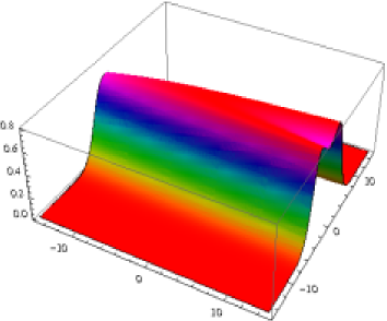
Figure 1: Dynamics of the exact soliton solution (39) for the potential field $|u(x,t)|$ of the generalized Lenells-Fokas equation (21). The unusual shape change and bending of the soliton indicates its decelerating motion with time-dependent velocity $v_{d}(t)$.

Note that (39) gives a more general soliton solution of the LF equation, where for the particular choice of the parameters with constant values: $c(t)=0$ and $a(t)=1,$ one recovers exactly the constant velocity soliton found in [11]. This demonstrates that we can extract the same soliton solution of the LF equation by just deforming the parameters of the known soliton [10] of the DNLS equation and thus can avoid the use of sophisticated methods like the RH or the dressing method [11, 12].

Another significant achievement is to construct in the same simple way the soliton solutions for all higher deformed LF equations by an easy extension of the time-dependence of the known DNLS or the LF soliton. For example, for the first higher deformation of the LF equation given by the higher nonlinear extension (26), the soliton solution can be expressed again in the form (39), with similar expressions for

$$\sigma=\xi x+2\omega(t),\ \theta=\eta(x-2v(t))$$

where the time-dependence of the parameters should be given now in a more extended form

$$\omega(t)=2Re(\Phi(\lambda_{1})),\ v(t)=\frac{2}{\eta}Im(\Phi(\lambda_{1})),$$

$$\mbox{where}\ \Phi(\lambda_{1})=\alpha\lambda^{2}_{1}t-\int^{t}dt^{\prime}(g_{0}(t^{\prime})+\frac{a_{0}(t^{\prime})}{\lambda_{1}^{2}}+\frac{c(t^{\prime})}{\lambda_{1}^{4}}),$$ (41)

in comparison with the LF soliton (36). The arbitrary time dependent functions $g_{0}(t)$ and $a_{0}(t)$ are asymptotic values of the perturbing functions $g(x,t)$ and $a(x,t)$ as in (25), respectively and can naturally be taken also as constant parameters.

Similarly, the N-soliton solution of the LF equation can be obtained avoiding the involved methods of [11, 12], by deforming the known N-soliton of the undeformed DNLS equation [10] using (33) with the choice $N_{+}=2,N_{-}=2$, which corresponds to the LF equation. We are however not going to reproduce here these otherwise simple steps.

B. Accelerating soliton in the deformed DNLS equation

As we have stated, the soliton solutions for the integrable nonholonomic deformation of the DNLS equation can be derived using general techniques like IST, Hirota’s bilinearization etc. or by the RH and the dressing method as done in [11, 12]. However we find them here in the simplest way by deforming the well known DNLS solitons already obtained in [10] through the ISM. We start therefore from the known undeformed soliton (43) and deform just its parameters like frequency and the velocity using (36) or (38), as we done for extracting the LF soliton. Thus we derive the 1-soliton for the deformed DNLS equation (30-19) or equivalently for (31), again in the form (37) yielding

$$|q|=\frac{2\sqrt{2}\eta}{(\cos\theta+\cos\gamma)^{\frac{1}{2}}}$$ (42)

with the only difference that the undeformed parameters like the initial frequency and the velocity (6) are given now as in the original DNLS soliton [10]:

$$\omega_{0}=2Re(\lambda^{4}_{1})=2(\xi^{2}-\eta^{2})=2\Delta^{4}\cos 2\gamma,\ \ v_{0}=2Im(\lambda^{4}_{1})/\eta=4\xi=4\Delta^{2}\cos\gamma.$$ (43)

The deformed DNLS soliton (42) as shown in Fig. 2a may exhibit again accelerated or decelerated motion, similar to the LF case depicted in Fig. 1, but with a difference in their initial velocities $v_{0}$. It is important to note here, that the perturbing functions $g,w$, which maintain the integrability of the system are not any given functions as in the usual perturbation theory, but are determined consistently through internal dynamics and can be expressed for the present models through the potential field $u(x,t)$ as (20). Therefore for the soliton solution (39) of the basic field these perturbing functions also take the solitonic form, which for the LF and the deformed DNLS equations in particular is as

$$w(x,t)=2ia(t)u$$ (44)

expressed through the solution (39) for the potential field $u(x,t)$ and similarly using (40):

$$g(x,t)=2\epsilon a(t)|u|^{2}+c(t)=c(t)+8\epsilon a(t)\frac{\sin^{2}\gamma}{\cosh^{2}2\theta-\sin^{2}\frac{\gamma}{2}},$$ (45)

graphical representation of which is given in Fig. 2b. Note that $w(x,t)$ is a complex function with soliton solution (44), while $g(x,t)$ is a real function with solution (45), both having time-dependent velocity $v(t)$ and frequency $\omega(t)$ as in (38), but additionally with a time-dependent amplitude $a(t)$. It should be noticed that, while at space infinities the perturbing function $w$ vanishes, $g$ goes to a time-dependent asymptotic $c(t)$, and drives the solitons from the space-boundaries. In this way the perturbing functions, themselves being consistent soliton solutions, preserve the integrability of the system and can force the basic field soliton to accelerate or decelerate. Such perturbations thus can play potentially important role in practical applications as we discuss later.

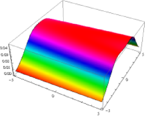
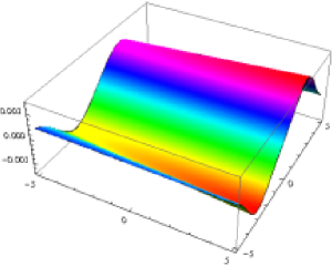
a)                                                            b)

Figure 2: Exact accelerating solitons in the nonholonomic deformation of the DNLS equation. a) Soliton for the basic field $|q|$ corresponding to (37) with (43). b) Consistent solitonic form (45) for the perturbing field $g(x,t)$ expressed through the potential field $|u(x,t)|^{2}$. Notice the nontrivial boundary value of the perturbed function.

The higher N-soliton of the nonholonomic deformation of the DNLS equation can similarly be derived by deforming the known N-soliton of the standard DNLS equation [10]. Likewise the solutions of all integrable equations in the deformed hierarchy can be obtained from those of the original undeformed integrable hierarchy by suitable deformation of the solitonic parameters as described above. In such deformed hierarchies, for every fixed $N_{+}$, one may choose $N_{-}$ as any even integer values, like $N_{-}=2,4$, as we have considered above, generating thus a novel two-fold hierarchy.

VIII. NONHOLONOMIC DEFORMATION OF THE CLL EQUATIONS, ITS TWO-FOLD HIERARCHY AND ACCELERATING SOLITONS

The CLL equation is another form of integrable derivative NLS equation with a different type of nonlinearity [13]. Following our approach as applied above for the deformed DNLS equation, we construct here the integrable nonholonomic deformation for the CLL equation.

A. Integrable CLL equation and soliton solution

The well known CLL equation given as

$$i\psi_{t}-\psi_{xx}+i2\epsilon|\psi|^{2}\psi_{x}=0,$$ (46)

shares all the rich properties of an integrable system, like commuting higher conserved quantities, integrable hierarchy, Lax pair and exact soliton solutions. Moreover due to its canonical Poisson bracket structure this system allows an exact quantum formulation with the algebraic Bethe ansatz solution [15]. It is important to note that the CLL equation is gauge related to the DNLS equation [16] and therefore it is intriguing in the present context to find the nonholonomic deformation of the CLL equation and examine how the gauge connection affects its relation with the deformed DNLS derived above.

Since our approach for nonholonomic deformation starts with the Lax pair we derive them from those of the DNLS system through a gauge transformation

$$U_{CLL}(\lambda)=h^{-1}U_{dnls}(\lambda)h-h^{-1}h_{x},\ V_{CLL}(\lambda)=h^{-1}V_{dnls}(\lambda)h-h^{-1}h_{t}.$$ (47)

where the gauge field is defined as

$$h=e^{i\delta(x,t)\sigma^{3}},\ \mbox{ with}\ \delta_{x}=\epsilon|q|^{2}=\epsilon|\psi|^{2},\ \ \delta_{t}=i\epsilon(\psi^{*}\psi_{x}-\psi\psi^{*}_{x})+6|\psi|^{4}.$$ (48)

Using the expressions (2) and (3) we can write down explicitly the CLL Lax pair, the flatness condition of which would generate the CLL equation (46). For example, the associated space-Lax operator, which is crucial for the ISM application, would take the form

$$U_{CLL}(\lambda)=-i(\lambda^{2}+\epsilon|\psi|^{2})\sigma_{3}+\lambda(\psi\sigma^{+}+\epsilon\psi^{*}\sigma^{-}).$$ (49)

One can carry out the ISM independently for extracting the soliton solution for this equation, which however can be avoided by noticing a direct relation between the CLL field $\psi$ and the DNLS field $q$ given by the gauge connection as

$$\ \psi=qe^{-i\delta(x,t)},\ \ \delta(x,t)=\epsilon\int^{x}|q|^{2}dy=\epsilon\int^{x}|\psi|^{2}dy,$$ (50)

which constructs the CLL soliton from (5) and (42) as

$$\psi=4\epsilon\eta\frac{\exp(2\theta-2i\sigma)}{\exp(4\theta)+\exp(i\epsilon\gamma)},$$ (51)

with the same expressions (6) for $\theta,\sigma$ and (43) for the unperturbed parameters $\omega_{0}$ and $v_{0}$. The soliton solution under nonholonomic deformation, as we see below, can be obtained by deforming the solitonic parameters (51) in the same way as done above.

B. Nonholonomic deformation of the CLL equation and accelerated soliton solution

For constructing the deformed CLL equation we follow the above procedure by taking the space-Lax operator $U_{CLL}(\lambda)$ as (49), while adding a deforming part (14) to the time-Lax operator $V_{CLL}(\lambda)$. The deforming matrices $G^{(j)},\ j=0,1,2$ may be taken in the same form (16), though due the gauge transformation they are linked in this case to (16) as $G^{(j)}\to h^{-1}G^{(j)}h$. Using therefore the deformed Lax operators we can derive the integrable perturbed CLL equation as

$$i\psi_{t}-\psi_{xx}+2i\epsilon|\psi|^{2}\psi_{x}=2(g\psi-iw),$$ (52)

and its complex conjugate, together with a different set of nonholonomic constraints on the perturbing functions:

$$g_{x}(x,t)=i{\epsilon}(\psi w^{*}-\psi^{*}w),\ w_{x}(x,t)=2ia(t)\psi-i\epsilon|\psi|^{2}w,$$ (53)

where $w$ in fact is gauge related to (19) through a transformation like (50). It is crucial to notice here that, in spite of the gauge equivalence between the unperturbed DNLS and the CLL equations, their respective nonholonomic deformations exhibit different structures as evident from (53). As a result the resolution of the constraints (53) by introducing the potential field, as done for the deformed DNLS, clearly fails here, since in $w_{x}$ as seen from (53) an extra term appears due to the gauge transformation. Therfore unlike the LF equation or the deformed DNLS discussed above, the perturbing fields can not be eliminated from the deformed set of the CLL equations (52)-(53) through the local potential field and one has to consider (52) as the perturbed CLL equation with nonholonomic constraints (53). The whole perturbed system however remains integrable with the associated Lax pair defined as above. The soliton solution for this deformed CLL equation takes again the form (51), where the expressions for $\theta,\sigma$ should be replaced as (38). Note that the unperturbed parameters are given here as (43), while the time-dependent deformed frequency $\omega_{d}(t)$ and the soliton velocity $v_{d}(t)$ are in the form (38). This would result again to an accelerating soliton, where the solution $|\psi|$ is the same as that for the deformed DNLS case $|q|$, shown in Fig. 2a. It is important to note here that in the above constraint relations (53), we have considered the same solution (16), which however is the simplest possible solution in the present case. The deforming matrix $G^{(2)}$ in fact can have a more general structure with nontrivial off-diagonal elements expressed through the function $e^{\delta(x,t)}$ defined in (50), since the last constraint in (15) is extended now to a more general form: $G^{(2)}_{x}+i\epsilon|\psi|^{2}[\sigma^{3},G^{(2)}]=0$. This situation would naturally make the constraint (53) more complicated, yielding another novel integrable perturbation of the CLL equation.

Exploiting the integrability of the deformed CLL equation we can construct its two-fold integrable hierarchy including the higher deformations, following the same recipe as above for the deformed DNLS equations. For this we can use again the same space-Lax operator (49) and construct the generalized time-Lax operator (12, 13) from those of the corresponding deformed DNLS by using the known gauge transformation (47,48). Note however that the higher order nonholonomic constraints on the deforming matrices $G^{(j)},\ j=0,1,2,\ldots$ are no longer same as (10), though may be derived from it through the gauge transformation (48), inducing the changes like

$$G^{(j)}\to h\tilde{G}^{(j)}h^{-1},\ \ G^{(j)}_{x}\to h(\tilde{G}^{(j)}_{x}+[h^{-1}h_{x},\tilde{G}^{(j)}])h^{-1}.$$

We however will not reproduce here such hierarchical equations explicitly.

IX. CONCLUDING REMARKS

The integrable nonholonomic deformation of the Kaup-Newell class including the derivative NLS equation, which remained as a challenging unsolved problem has been solved here completely with the construction of a two-fold integrable hierarchy with higher order deformations. As an important application we identify the recent Lenells-Fokas equation as a member of this deformed DNLS hierarchy, which allows us to bypass the involved procedures of [11, 12] and find its soliton solution as a simple deformation of the known DNLS soliton. The soliton solutions in such deformed systems are shown to exhibit unusual properties like accelerating (decelerating) solitonic motion, induced by the perturbing functions, which control such motions from the space-boundaries.

The nonholonomic deformation of the Chen-Lee-Liu derivative NLS equation though can be constructed similarly, gauge relation between the undeformed CLL with the Kaup-Newell DNLS equation, is not extended straightforwardly to their corresponding deformed equations. Nevertheless the soliton solution of the deformed CLL equation together with that for its deformed hierarchy can be constructed in a similar way.

A promising potential application of the nonholonomic deformation for the family of DNLS equations arises when such deformations are interpreted as perturbations subjected to differential constraints, which keep the whole system integrable. Such perturbed DNLS equation can be considered therefore as a novel coupled system of the DNLS and a Maxwell-Bloch type equation and may have important applications in the fiber optics communication boosted by a doped laser system, extending the idea of [17] to a new direction [18].

References

- [1] C. S. Gardner, J. M. Green, M. D. Kruskal and R. M. Miura, Phys. Rev. Lett. 19, 1095 (1967)
- [2] A. Karasu-Kalkanli, A. Karasu, A. Sakovich, S. Sakovich, R. Turhan, J. Math. Phys. 49, 073516 (2008)
- [3] B. A. Kupershmidt, Phys. Lett., A 372, 2634 (2008)
- [4] A. Kundu, J. Phys. A 41, 495201 (2008)
- [5] Y. Yad and Y. Zeng, eprint: arXiv:0810.1986 [nlin.SI] (2008)
- [6] A. Kundu, J. Math. Phys. 50, 1 (2009)
- [7] A. Kundu, R. Sahadevan and L. Nalinidevi, J. Phys. A 42, 115213 (2009)
- [8] Z. Qiao and W. Strampp, Physica A 313, 365 (2002)
- [9] J. F. Gomes, G. S. Franca, G. R. de Melo and A. H. Zimerman, eprint: arXiv:0906.5579 [hep-th] (2009)
- [10] D. J. Kaup and A. C. Newell, J. Math. Phys. 19, 798 (1978)
- [11] J. Lenells and A.S. Fokas, Nonlinearity 22 11 (2009)
- [12] J. Lenells, eprint: arXiv:0909.3021 [nlin.SI] (2009)
- [13] H. H. Chen, Y. C. Lee and C. S. Liu, Phys. Scripta 20, 490 (1979)
- [14] J. Lenells, Stud. Appl. Math. 123, 215 (2009)
- [15] A. Kundu and B. Basu Mallick, J. Math. Phys. 34, 1252 (1993)
- [16] A. Kundu, J. Math. Phys. 25, 3433 (1984)
- [17] A. I. Maimistov and E. A. Manyakin, Sov. Phys. JETP 58, 685 (1983); S. Kakei and J Satsuma, J. Phys. Soc. Jpn. 63, 885 (1994)
- [18] A. Kundu (under preparation)