Markovian embedding of non-Markovian superdiffusion

Abstract

We consider different Markovian embedding schemes of non-Markovian stochastic processes that are described by generalized Langevin equations (GLE) and obey thermal detailed balance under equilibrium conditions. At thermal equilibrium superdiffusive behavior can emerge if the total integral of the memory kernel vanishes. Such a situation of vanishing static friction is caused by a super-Ohmic thermal bath. One of the simplest models of ballistic superdiffusion is determined by a bi-exponential memory kernel that was proposed by Bao [J.-D. Bao, J. Stat. Phys. 114, 503 (2004)]. We show that this non-Markovian model has infinitely many different 4-dimensional Markovian embeddings. Implementing numerically the simplest one, we demonstrate that (i) the presence of a periodic potential with arbitrarily low barriers changes the asymptotic large time behavior from free ballistic superdiffusion into normal diffusion; (ii) an additional biasing force renders the asymptotic dynamics superdiffusive again. The development of transients that display a qualitatively different behavior compared to the true large-time asymptotics presents a general feature of this non-Markovian dynamics. These transients though may be extremely long. As a consequence, they can be even mistaken as the true asymptotics. We find that such intermediate asymptotics exhibit a giant enhancement of superdiffusion in tilted washboard potentials and it is accompanied by a giant transient superballistic current growing proportional to $t^{\alpha_{{\rm eff}}}$ with an exponent $\alpha_{\rm eff}$ that can exceed the ballistic value of two.

I Introduction

The subject of anomalous diffusion has become increasingly popular and important in the last years with a number of papers growing faster than linearly in time with almost 500 papers published last year. There also is a large number of theoretical models that lead to anomalous diffusion such as as continuous time-random walks Scher ; Shlesinger ; Hughes ; Bouchaud , including Levy flights and Levy walks Hughes ; Metzler , related fractional Fokker-Planck equations MetzlerPRL ; Metzler and (ordinary) Langevin equations in random subordinated time Fogedby ; Stanislavsky , as well as (ordinary) Langevin equations with additive non-Gaussian Levy white noises Ditlevsen ; Dubkov . Moreover nonlinear Brownian motion with multiplicative Gaussian white noise Marksteiner ; LutzPRL , as well as linear Boltzmann equation with scattering events being distributed in time according to a power law distribution BarkaiSilbey ; Friedrich may display anomalous diffusion. This list by far is not complete. Yet the quest for minimal and fundamental physical models has become ever more important. One of the fundamental approaches to anomalous diffusion Wang ; Morgado ; Pottier ; WeissBook is provided by the generalized Langevin equation (GLE) Kubo ; Bogolyubov ; Zwanzig ; HTB90 with a frictional memory kernel $\gamma(t)$, reading:

$$m\ddot{x}+m\int_{0}^{t}\gamma(t-t^{\prime})\dot{x}(t^{\prime})dt^{\prime}+\frac{\partial V(x,t)}{\partial x}=\zeta(t)\;,$$ (1)

where $x(t)$ denotes the position of a particle of mass $m$. Here $\zeta(t)$ is a Gaussian zero-mean fluctuating force that at temperature $T$ is related to the memory kernel by the fluctuation-dissipation relation Kubo

$$\langle\zeta(t)\zeta(t^{\prime})\rangle=k_{B}Tm\gamma(|t-t^{\prime}|)\;.$$ (2)

Remarkably, this model can be derived from a Hamiltonian dynamics of a particle that bilinearly couples with coupling constants $c_{i}$ to a thermal bath of harmonic oscillators with masses $m_{i}$ and frequencies $\omega_{i}$, $H_{B,\rm int}(p_{i},q_{i},x)=(1/2)\sum_{i}\{p_{i}^{2}/m_{i}+m_{i}\omega_{i}^{2}[q_{i}-c_{i}x/(m_{i}\omega_{i}^{2})]^{2}\}$. The total effect of the bath oscillators, which are initially canonically distributed with $H_{B,\rm int}$ at temperature $T$ and fixed $x=x(0)$, is characterized by the bath spectral density

$$J(\omega)=\frac{\pi}{2}\sum_{i}\frac{c_{i}^{2}}{m_{i}\omega_{i}}\delta(\omega-\omega_{i}).$$ (3)

It is related to the power spectral density of the fluctuating force

$$S(\omega)=\int_{-\infty}^{\infty}\langle\zeta(\tau)\zeta(0)\rangle e^{-i\omega\tau}d\tau$$ (4)

via $S(\omega)=2k_{B}TJ(\omega)/\omega$ Kubo ; HTB90 . This in general leads to a non-Markovian process of the particle dynamics with linear memory friction and Gaussian fluctuating force. Moreover, due to the fluctuation-dissipation relation (2) it is compatible with thermal equilibrium in confining, time-independent potentials and encompasses a whole set of physically meaningful models characterized by different bath spectral densities $J(\omega)$.

In the absence of any potential the variance of the particle’s position will grow with time. The law according to which the variance grows characterizes the nature of the resulting diffusion process as being subdiffusive if the growth of the variance is slower than linear. This happens if the static friction $\gamma=\int_{0}^{\infty}\gamma(t^{\prime})dt^{\prime}$ diverges. Normal diffusion corresponds to a linear growth. It occurs if $\gamma$ is finite. Finally, if $\gamma$ vanishes the variance grows faster than linear and one speaks of superdiffusion. The presence of a nonlinear time-dependent force $f(x,t)=-\partial V(x,t)/\partial x$ modifies this simple picture in a complicated way depending on further details of the memory kernel and also on temperature. The qualitative behavior of the variance of the position is determined by the variance of the velocity, $\langle\Delta v^{2}(t)\rangle$. The mean square displacement of position spreads according to normal diffusion, if the integral of the velocity variance over all times is finite. On the other hand if this integral is zero, then the motion is anti-persistent and subdiffusive. If this integral diverges the spread of the position variance is superdiffusive. For free motion in the absence of a potential these criteria are equivalent to those for the memory kernel which in general fail in the presence of a potential. Since general analytical results are scarce and most likely nonexistent for nonlinear and time-dependent forcing, the reliability of numerical simulations has become a key issue. Numerically tractable models can be obtained by approximating the given memory kernel by a finite sum of exponential functions. The according non-Markovian particle dynamics can then be obtained as the projection of a high-dimensional Markovian process onto the phase space of the particle spanned by the particle’s coordinate and momentum $p=m\dot{x}$. The dimensionality of the Markovian process is $D=N+2$, where $N$ is the number of exponentials in the sum approximating the memory kernel. The key point is that the corresponding Markovian dynamics can be propagated locally in time for very long time intervals by means of very reliable algorithms with a well controlled numerical precision. Moreover, this way of thinking allows one to identify the simplest models for the superdiffusive GLEs with minimal embedding dimensions $D=3$ and $D=4$. The case $D=4$ corresponds to approximating the memory kernel by a difference of two exponentials,

$$\gamma(t)=\gamma_{1}\exp(-k_{1}t)-\gamma_{2}\exp(-k_{2}t),$$ (5)

such that $\gamma_{1}/k_{1}=\gamma_{2}/k_{2}$ implying to vanishing static friction $\gamma$ and $\gamma_{1}>\gamma_{2}$. The latter condition amounts to the fact that the memory kernel is proportional to the autocorrelation function of the fluctuating force $\zeta$ and hence must be non-negative semidefinite. This bi-exponential model was proposed by Bao Bao04 . It corresponds to a super-Ohmic spectral density of thermal bath oscillators, $J(\omega)\propto\omega^{3}$ at low frequencies and describes the coupling of a particle to three-dimensional lattice phonons. It therefore models the diffusion of an impurity in a crystal. We will demonstrate that this model can be embedded in infinitely many ways. In the following we will study one of the simplest embeddings which is different from those used by Bao Bao04 ; Bao06 ; Bao05a . In the absence of any force $f(x,t)$ the spreading of the particle’s position distribution is ballistic, $\langle\Delta x^{2}(t)\rangle=D_{2}t^{2}$, and hence super-diffusive. Here and in the following, the expectation $\langle...\rangle$ refers to an ensemble average with respect to the fluctuating force $\zeta(t)$ and an initial distribution of position and momentum, $x(0)$ and $p(0)$, respectively. The velocity process is non-ergodic Bao05 . As a consequence, the ballistic superdiffusion coefficient $D_{2}$ turns out to depend on the initial velocity distribution. However, as we shall see below this non-ergodic feature disappears in periodic potentials. Moreover, our numerics reveals that the ballistic diffusion in tilted periodic potentials does neither depend on the initial velocity distribution, nor on the initially non-equilibrium noise preparation. For this reason, we presume that the velocity process of the particle then becomes ergodic.

The minimal, three-dimensional Markovian embedding of the GLE superdiffusion is achieved in the limit $\gamma_{1}\to\infty$, $k_{1}\to\infty$, so that $\gamma_{0}=\gamma_{1}/k_{1}={\rm const}=\gamma_{2}/k_{2}$. In this limit, the first exponential becomes a delta-function $2\gamma_{0}\delta(t)$. This case will be studied elsewhere.

Unfortunately, a non-Markovian Fokker-Planck-type equation (NMFPE) that corresponds to a GLE with a general, nontrivial potential is not known in spite of many years of search. The only exceptions are provided by (strictly) linear and parabolic potentials, where the corresponding NMFPEs were derived by Adelman Adelman and Hänggi hanggi ; hanggi2 ; hanggi3 for stable non-Markovian Brownian motion and, as well, for unstable non-Markovian dynamics hanggiUNM ; i.e. the Kramers problem of escape over a parabolic barrier HTB90 . Using the fact that $[x(t),\dot{x}=v(t)]$ is a two-component Gaussian process, which is obtained by a linear integral transformation of the Gaussian noise process $\zeta(t)$ the resulting NMFPE assumes the form of a time-dependent FPE. This FPE-structure of time-evolution for the single-time event probability of the non-Markovian process should then not be mistaken as an effective Markovian dynamics hanggi ; hanggi2 ; hanggi3 . Notwithstanding these exceptional known cases cases of non-Markovian Gaussian dynamics, this lack of a generally closed NMFPE for nonlinear forces lends even more importance to the Markovian embedding approach.

This paper is structured as follows. In Sec. II and Appendix I we detail the Markovian embedding procedure in a slightly more general way than has been used so far. The general results are illustrated with two different embeddings of one and the same superdiffusive GLE dynamics. In Sec. III, we present and discuss the results of stochastic simulations of superdiffusion under a constant bias and in a washboard potential for one of these embeddings. The issue of ergodicity of mean square displacement is discussed in Sec. IV. Conclusions are drawn in Sec. V.

II Method

The idea that we pursue here is to represent the non-Markovian stochastic dynamics of a single particle with $(x,p)$ phase space as a projection of a multi-dimensional Markovian dynamics. It is well known that any GLE can be derived from the (Markovian) Hamiltonian dynamics of a particle coupled to a thermal bath of harmonic oscillators. This Hamiltonian embedding though requires a large number of auxiliary degrees of freedom representing the thermal bath. Here we look for an embedding with a minimal number $N$ of auxiliary variables which all together constitute a continuous Markovian process. A low embedding dimension is crucial for running numerical simulations which can become extensively time-consuming for a large $N$.

We first rewrite the GLE (1) in terms of the phase space coordinates $x$ and $p=m\dot{x}$ as

$$\dot{x}(t)= \frac{1}{m}p(t)$$

$$\dot{p}(t)= f(x,t)-\int_{0}^{t}\gamma(t-t^{\prime})p(t^{\prime})dt^{\prime}+\zeta(t)\;.$$ (6)

The embedding involves a yet to be determined number $N$ of auxiliary dynamical variables collected into a vector $\vec{u}(t)$ in terms of which the dynamics takes the following general form

$$\dot{x}(t)= \frac{1}{m}p(t)$$

$$\dot{p}(t)= f(x,t)+\roarrow{g}^{\mathrm{T}}\roarrow{u}(t)$$

$$\dot{\roarrow{u}}(t)= -p(t)\roarrow{r}-\mathbf{A}\roarrow{u}(t)+\mathbf{C}\roarrow{\xi}(t)\;,$$ (7)

where $\roarrow{g}$ and $\roarrow{r}$ denote constant vectors of dimension $N$ and $\mathbf{A}$, and $\mathbf{C}$ are constant $N\times N$ matrices. The upper index $T$ denotes the transpose of a vector or a matrix. Further, $\roarrow{\xi}(t)$ is a vector of uncorrelated Gaussian white noises,

$$\langle\xi_{i}(t)\xi_{j}(t^{\prime})\rangle=\delta(t-t^{\prime})\delta_{ij}\;$$ (8)

with $N$ components. Integrating the equation for the auxiliary vector $\roarrow{u}(t)$ and substituting the result in the equation for the momentum $p(t)$ one recovers the original GLE (II) only under special conditions, see Appendix A for details of the derivation. First, the memory kernel $\gamma(t)$ must satisfy

$$\gamma(t)= \roarrow{g}^{\mathrm{T}}e^{-\mathbf{A}t}\roarrow{r}\;.$$ (9)

Since the right hand side can in general be represented as a sum of $N$ exponential functions $\exp(-\lambda_{i}t)$, $i=1\ldots N$ with the eigenvalues $\lambda_{i}$ of the matrix $\mathbf{A}$ the embedding can be exact only if the memory kernel is of the same type Jordan . But also other memory kernels such as algebraically decaying functions can be approximated by a finite sum of exponential functions, even with a relatively small extra dimension $N$, and hence are amenable to Markovian embedding.
Furthermore, the fluctuation-dissipation relation (2) imposes restrictions on the matrices $\mathbf{A}$, $\mathbf{C}$, and the vectors $\roarrow{g}$ and $\roarrow{r}$. These restrictions are met if the embedding parameters satisfy the following two relations:

$$\mathbf{G}\roarrow{g} =mk_{B}T\roarrow{r}$$ (10)

$$\mathbf{C}\mathbf{C}^{\mathrm{T}} =\mathbf{A}\mathbf{G}+\mathbf{G}\mathbf{A}^{\mathrm{T}}\;,$$ (11)

which defines the constant $N\times N$ matrix $\mathbf{G}$.
However, for arbitrary initial values of the auxiliary variables $\roarrow{u}(0)$, the fluctuation-dissipation relation will be obeyed only asymptotically. This means that the noise $\zeta(t)$ in Eq. (II) is initially nonstationary and becomes only gradually stationary in the course of time, see Appendix A, Eq. (44). In order to guarantee the Gaussian nature of the random force $\zeta(t)$ the vector $\roarrow{u}(0)$ must also be Gaussian distributed, see Eq.(39). Because the vector $\roarrow{u}(0)$ is independent of the vector of Gaussian white noises $\roarrow{\xi}(t)$ and its first moment must vanish, it is sufficient to specify its covariance matrix

$$\langle\roarrow{u}(0)\otimes\roarrow{u}^{\mathrm{T}}(0)\rangle=\mathbf{G}\;.$$ (12)

It must coincide with $\mathbf{G}$ in Eq. (10), in order to have the fluctuation-dissipation relation (2) obeyed for all times, see Eq. (44).

Yet the conditions (9), (10) and (11) do not uniquely determine the enlarged process and actually leave room for an infinite variety of different processes leading upon reduction to the same generalized Langevin equation. Since some of the enlarged processes allow faster and more reliable numerical simulations than others there is a great interest in identifying computationally optimal embeddings. We further note that the relations (9), (10) and (11) are sufficient but not necessary conditions. The resulting embedding is more general than previous ones such as those proposed in Refs. Kupferman ; Marchesoni which assume $\roarrow{r}=\roarrow{g}$.

Before discussing a particular example we would like to emphasize that the stationarity of the fluctuating force and the fluctuation dissipation relation (2) are exactly implemented.

II.1 Minimal model

We now consider the simple class of models specified by the bi-exponential memory kernel (5). Under the condition of vanishing static friction, i.e. $\gamma_{1}k_{2}=\gamma_{2}k_{1}$, this memory kernel is specified by three independent parameters that can be written as

$$\kappa^{2}=\gamma_{1}-\gamma_{2},\quad\nu=k_{1}+k_{2}\quad\textrm{and}\quad\omega_{0}^{2}=k_{1}k_{2}\;.$$ (13)

Note that $\kappa$ is always a real parameter due to the positivity constraint $\gamma_{1}>\gamma_{2}$. In terms of this parameterization the Laplace transform $\hat{\gamma}(s)$ of the memory kernel becomes

$$\hat{\gamma}(s)=\int_{0}^{\infty}e^{-st}\gamma(t)dt=\frac{\kappa^{2}s}{s^{2}+\nu s+\omega_{0}^{2}}\;.$$ (14)

One can now easily calculate the power spectral density, see Eq. (4), by connecting it to the friction kernel via the fluctuation-dissipation relation, see Eq. (2):

$$\begin{split}S(\omega)&=2k_{B}Tm\int_{0}^{\infty}\gamma(t)\cos(\omega t)dt\\ &=2k_{B}Tm\operatorname{Re}\big{(}\hat{\gamma}(i\omega)\big{)}\\ &=\frac{2k_{B}Tm\kappa^{2}\nu\omega^{2}}{(\omega^{2}-\omega_{0}^{2})^{2}+\nu^{2}\omega^{2}}\;.\end{split}$$ (15)

It is interesting to note that the power spectral density has a maximum at the frequency $\omega_{0}$.

There are several possibilities to realize Markovian embedding of this non-Markovian model. In the following we shall discuss two of them.

II.1.1 First embedding

A simple embedding is obtained by choosing:

$$\begin{split}\mathbf{A}&=\left(\begin{array}[]{cc}\nu&\omega_{0}\\ -\omega_{0}&0\\ \end{array}\right)\\ \roarrow{g}^{T}&=\roarrow{r}^{T}=\left(\kappa,\;0\right)\\ \mathbf{C}&=\sqrt{2mk_{B}T\nu}\left(\begin{array}[]{cc}1&0\\ 0&0\\ \end{array}\right)\\ \langle u_{i}(0)&u_{j}(0)\rangle=mk_{B}T\delta_{ij}\;.\end{split}$$ (16)

This choice leads to the following equations:

$$\begin{split}\dot{x}(t)=&\frac{1}{m}p(t)\\ \dot{p}(t)=&-\frac{\partial}{\partial x}V(x,t)+\kappa u_{1}(t)\\ \dot{u}_{1}(t)=&-\kappa p(t)-\nu u_{1}(t)-\omega_{0}u_{2}(t)\\ &+\sqrt{2mk_{B}T\nu}\xi(t)\\ \dot{u}_{2}(t)=&\omega_{0}u_{1}(t)\;,\end{split}$$ (17)

where $\xi(t)$ is scalar Gaussian white noise. Moreover, this embedding also allows for complex parameters $k_{1}=k_{2}^{*}$, providing the possibility to model oscillating real valued kernels

$$\gamma(t) = \kappa^{2}e^{-\nu t/2}[\cos(t\sqrt{\omega_{0}^{2}-\nu^{2}/4})$$

$$- \frac{\nu}{\sqrt{4\omega_{0}^{2}-\nu^{2}}}\sin(t\sqrt{\omega_{0}^{2}-\nu^{2}/4})]\;.$$

This model corresponds to sharply peaked power spectral density $S(\omega)$, and bath spectral density $J(\omega)$.

II.1.2 Second embedding

An alternative way is to start with a diagonal matrix $\mathbf{A}$. It would be tempting to also choose diagonal matrices $\mathbf{C}$ and $\mathbf{G}$. This choice though always yields a linear combination of exponential functions with positive coefficients for the memory kernel (5) Goychuk09 and hence does not allow vanishing static friction. However, this goal can be achieved by means of the following choice of parameters involving non-diagonal matrices $\mathbf{C}$ and $\mathbf{G}$

$$\begin{split}\mathbf{A}&=\left(\begin{array}[]{cc}k_{1}&0\\ 0&k_{2}\\ \end{array}\right)\\ g_{1,2}&=\sqrt{\gamma_{1,2}\frac{k_{1}+k_{2}}{k_{1}-k_{2}}}\\ r_{1,2}&=\sqrt{\gamma_{1,2}\frac{k_{1}-k_{2}}{k_{1}+k_{2}}}\\ \mathbf{C}&=\sqrt{2mk_{B}T}\left(\begin{array}[]{cc}\sqrt{k_{1}}&0\\ -\sqrt{k_{2}}&0\\ \end{array}\right)\\ \mathbf{G}&=mk_{B}T\left(\begin{array}[]{cc}1&-c\\ -c&1\\ \end{array}\right)\;,\end{split}$$ (19)

where $0<c=2\sqrt{k_{1}k_{2}}/(k_{1}+k_{2})<1$ is the correlation coefficient of the covariance matrix $\mathbf{G}$ and $k_{1}=k_{2}(\gamma_{1}/\gamma_{2})>k_{2}$. This choice is similar to the one in Bao04 . We note that the second embedding requires that the parameters $k_{1}$ and $k_{2}$ must be real. Therefore it is not possible to model an oscillating kernel by this method. Our first embedding in Eq. (17) is, however, simpler and numerically more convenient since its numerical simulation requires less operations. For instance, only one stochastic variable has to be generated in the first embedding scheme, see Eq. (16), in contrary to two, needed in the second embedding scheme, see. Eq.(19). All this makes our first embedding scheme preferential.

II.2 Dimensionless units

For further studies, we transform Eq. (17) into dimensionless units by scaling momentum in terms of thermal momentum $p_{T}=\sqrt{mk_{B}T}$, expressing the distance in terms of a typical length scale some arbitrary length $x_{0}$, which becomes the spatial period for periodic potentials (see below) and time in units of $\tau_{0}=x_{0}/v_{T}$. The auxiliary variables $u_{1}$ and $u_{2}$ are scaled in units of $u_{0}=mx_{0}/(\kappa\tau^{2}_{0})$. The energy is scaled in units of $k_{B}T$. This yields the equations of motion

$$\dot{\tilde{x}}= \tilde{v}$$

$$\dot{\tilde{v}}= -\frac{\partial}{\partial\tilde{x}}\tilde{V}(\tilde{x},\tilde{t})+\tilde{u}_{1}$$

$$\dot{\tilde{u}}_{1}= -\tilde{\kappa}^{2}\tilde{v}-\tilde{\nu}\tilde{u}_{1}-\tilde{\omega}_{0}\tilde{u}_{2}+\tilde{\kappa}\sqrt{2\tilde{\nu}}\xi$$

$$\dot{\tilde{u}}_{2}= \tilde{\omega}_{0}\tilde{u}_{1}\;,$$ (20)

which were used in our simulations. Here, $\tilde{\kappa}=\kappa\tau_{0}$, $\tilde{\omega}_{0}=\omega_{0}\tau_{0}$, $\tilde{\nu}=\nu\tau_{0}$. All results in the following figures are given in these dimensionless units.

III Results

The numerical results presented below were obtained using the standard stochastic Euler method Gard . A Mersenne Twister pseudo random number generator was used to produce uniformly distributed random numbers which were transformed into Gaussian variables using Box-Muller algorithm NumRec . Typically, an ensemble of $n=10^{4}$ particles (or trajectories) was propagated in time with a fixed time step between $\Delta t=10^{-4}$ and $10^{-5}$ in most simulations to achieve (weak) convergence of ensemble averaged results. The use of double precision thus cannot be avoided and reliable numerics are very time consuming. All the particles were initially localized at $x(0)=0$ with the initial velocities sampled from some probability distribution. In most simulations we assumed this distribution to be sharply peaked at zero and ascribed zero initial velocities to all the particles, although the thermal Maxwellian distribution was also used. The auxiliary variables $u_{i}(0)$ were (mostly) sampled from the corresponding Gaussian distributions to achieve at the exact equivalence of the simulated Markovian dynamics to that of GLE, as described in the Section II. Method. Sometimes, we used also a different initial distribution of $u_{i}(0)$ (all equal zero) in order to clarify the influence of the initially non-equilibrium noise preparation on the stochastic dynamics. In all cases, we denote the corresponding ensemble averages as $\langle...\rangle$ and specify the initial distributions if not obvious.

Of central interest are the first moment $\langle\Delta x(t)\rangle$ and the variance $\langle\Delta x^{2}(t)\rangle$ of the displacement

$$\Delta x(t)=x(t)-x(0)=\int_{0}^{t}dt^{\prime}v(t^{\prime}).$$ (21)

Accordingly we have

$$\langle\Delta x(t)\rangle=\int_{0}^{t}dt^{\prime}\langle v(t^{\prime})\rangle$$ (22)

and

$$\begin{split}\langle\Delta x^{2}(t)\rangle&=\langle(\Delta x(t)-\langle\Delta x(t)\rangle)^{2}\rangle\\ &=\int_{0}^{t}\int_{0}^{t}dt_{1}dt_{2}C_{v}(t_{1},t_{2})\;,\end{split}$$ (23)

where $C_{v}(t_{1},t_{2})$ denotes the velocity fluctuation autocorrelation function

$$C_{v}(t_{1},t_{2})=\langle(v(t_{1})-\langle v(t_{1})\rangle)(v(t_{2})-\langle v(t_{2})\rangle)\rangle\;.$$ (24)

These quantities were estimated on the basis of averages over the ensemble of simulated particle trajectories.

Of particular interest will turn out the question under which conditions the process of velocity fluctuations defined as the deviation of velocity from its mean value constitutes an ergodic process Deng ; Papoulis . The definition and main properties of an ergodic process are collected in Appendix B.

III.1 Superdiffusion in presence of a constant bias

First, we consider the Langevin dynamics (1) with an arbitrary memory kernel under a constant biasing force $F$, i.e with $V(x,t)=-Fx$. This special biased problem is analytically solvable, cf. Wang ; Morgado ; Pottier ; Kupferman , and therefore provides a suitable test of our numerical simulations. The mean square displacement in this case does not depend on the external bias $F$ and is given by: $\langle\Delta x^{2}(t)\rangle=\langle x^{2}(t)\rangle-\langle x(t)\rangle^{2}$ becomes

$$\langle\Delta x^{2}(t)\rangle=2v_{T}^{2}\int_{0}^{t}H(t^{\prime})dt^{\prime}+\left[\langle v^{2}(0)\rangle-v_{T}^{2}\right]H^{2}(t),$$ (25)

where we denote the thermal average of initial velocities by $v_{T}^{2}\equiv\langle v^{2}(0)\rangle_{T}=k_{B}T/m$ and

$$H(t)=\int_{0}^{t}K_{v}(\tau)d\tau$$ (26)

is the integral of the (normalized) equilibrium autocorrelation function of the velocity fluctuations which is defined as

$$K_{v}(\tau)=C_{v}(\tau,0)/v^{2}_{T}\;.$$ (27)

It has the Laplace-transform

$$\hat{K}_{v}(s)=\frac{1}{s+\hat{\gamma}(s)}\;.$$ (28)

We note that the velocity fluctuations present a wide sense ergodic process if and only if the time average of $K_{v}(t)$ vanishes, i.e.:

$$\lim_{t\to\infty}\frac{1}{t}H(t)=0,$$ (29)

see also Appendix B. For the mean displacement one obtains

$$\langle\Delta x(t)\rangle=\frac{F}{m}\int_{0}^{t}H(t^{\prime})dt^{\prime}.$$ (30)

If one chooses thermally distributed initial velocities, $\langle v^{2}(0)\rangle=v_{T}^{2}$, then the first and second moments of the displacement are connected by the fluctuation-dissipation theorem (FDT)

$$\langle\Delta x(t)\rangle=\frac{F}{2k_{B}T}\langle\Delta x^{2}(t)\rangle,$$ (31)

for any memory kernel. Notice that the mass of the particle is not involved in Eq. (31). Provided that the velocity process is ergodic in the wide sense the second term on the right hand side of Eq. (25) can be neglected compared to the first term if time goes to infinity. Hence, for an ergodic velocity process the spreading of the particle position becomes independent of the initial velocity distribution. In contrast, for a nonergodic process the second term can become comparable in magnitude or even dominant for large times. Then the influence of the initial velocity distribution on the second moment of the position survives. This actually happens if the Laplace transform of the memory kernel, $\hat{\gamma}(s)$ approaches zero for $s\to 0$ proportionally to $s$ or faster. In this case, the FDT (31) is not valid for $\langle v^{2}(0)\rangle\neq v_{T}^{2}$, even asymptotically.

As an example we consider the minimal model (5). Its Laplace transform indeed vanishes linearly with $s\to 0$, see Eq. (14). For the Laplace transform of the velocity correlation coefficient one obtains from Eq. (28)

$$\hat{K}_{v}(s)=\frac{s^{2}+\nu s+\omega_{0}^{2}}{s(s^{2}+\nu s+w_{0}^{2}+\kappa^{2})}\;.$$ (32)

Inverting the Laplace transform, one obtains for the velocity correlation coefficient

$$K_{v}(\tau) = \frac{\omega_{0}^{2}}{\omega_{0}^{2}+\kappa^{2}}+\frac{\kappa^{2}}{\omega_{0}^{2}+\kappa^{2}}e^{-\nu\tau/2}$$

$$\times \Big{[}\cosh(\frac{\sqrt{\nu^{2}-4\omega_{0}^{2}-4\kappa^{2}}}{2}\tau)$$

$$+ \frac{\nu}{\sqrt{\nu^{2}-4\omega_{0}^{2}-4\kappa^{2}}}\sinh(\frac{\sqrt{\nu^{2}-4\omega_{0}^{2}-4\kappa^{2}}}{2}\tau)\Big{]}\;.$$

Note that with $\lim_{\tau\to\infty}K_{v}(\tau)=\omega_{0}^{2}/(w_{0}^{2}+\kappa^{2})$ the equilibrium autocorrelation function of velocity fluctuations as well as its time average attain positive values. This confirms that the velocity process of the minimal model is nonergodic in the case of linear potentials.

The mean square displacement of the position can be exactly evaluated by means of Eq. (25). We refrain from presenting the resulting lengthy expression and only compare the such derived exact result with the mean square displacement obtained from a simulation of the Markovian model via the first embedding for a particular set of parameters, see Fig. 1. The agreement between the analytical result and the simulation is very good.

For short times the spreading of the mean square displacement of the position becomes

$$\langle\Delta x^{2}(t)\rangle = \langle v^{2}(0)\rangle t^{2}$$ (34)

$$+ \kappa^{2}\left[3v_{T}^{2}-4\langle v^{2}(0)\rangle\right]t^{4}/12+O(t^{5}).$$

For a strictly vanishing initial velocity the contribution proportional to $t^{2}$ disappears and the diffusion initially becomes super-ballistic with $\langle\Delta x^{2}(t)\rangle\propto t^{4}$, see Fig. 1. Otherwise, the diffusion initially is ballistic. For large times ballistic diffusion results with $\langle\Delta x^{2}(t)\rangle\sim D_{2}t^{2}$. Due to the nonergodicity of the velocity process the ballistic superdiffusion coefficient $D_{2}$ depends on the initial distribution of velocities,

$$D_{2} = v_{T}^{2}\frac{\omega_{0}^{2}}{\omega_{0}^{2}+\kappa^{2}}$$ (35)

$$\times \left[1+\left(\frac{\langle v^{2}(0)\rangle}{v_{T}^{2}}-1\right)\frac{\omega_{0}^{2}}{\omega_{0}^{2}+\kappa^{2}}\right]\;.$$

Fig. 1 also displays simulation results of the first embedding for vanishing initial values of the auxiliary variable, i.e. $u_{1}(0)=u_{2}(0)=0$, and also for initial values from a Gaussian distribution with variance $\langle u_{i}(0)u_{j}(0)\rangle=\kappa^{2}\delta_{i,j}$. We recall that the latter choice guarantees that the fluctuating forces are stationary and that they satisfy the fluctuation-dissipation relation (2). The mean square displacement resulting from zero initial auxiliary variables is remarkably different from that with the correct Gaussian distributed initial auxiliary variables not only at short times but also for large times where it approaches normal instead of ballistic diffusion. The strong influence of the initial conditions even at large times is another consequence of the non-ergodicity of the velocity. In contrast, for an ergodic velocity process the long time behavior of the position mean square displacement has lost any memory on initial conditions.

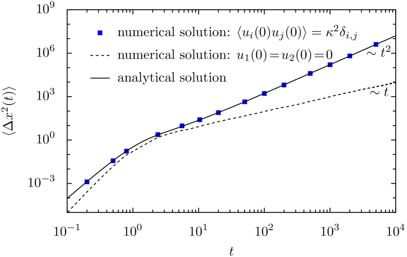
Figure 1: (Color online) The mean square displacement of the position (being independent of the bias $F$) as a function of time changes from a $t^{4}$ law at small times to a ballistic $t^{2}$ law. Comparison of the analytical solution according to Eq. (25) (solid line) and results from numerical simulations of the first embedding (square symbols) exhibit good agreement. A strongly deviating result is obtained if the auxiliary variables of the first embedding initially assume vanishing values (dashed line). The other parameters $\kappa=2$, $\nu=3$, $\omega_{0}=1$ and $v(0)=0$ are the same for the displayed curves. The estimate of the mean square displacement is obtained by an average over an ensemble of $10^{4}$ simulated trajectories.

III.2 Superdiffusion in a washboard potential

Next we consider the diffusion in a periodic washboard potential $V(x,t)=-V_{0}\cos(2\pi x/x_{0})$ of spacial period $x_{0}$. Here no analytical results are available, instead we performed numerical simulations of the first embedding. In Fig. 2 we compare the simulated mean square displacement as a function of time for different heights of the potential barriers separating neighboring periods of the potential. After a short initial period of fast growth the diffusion turns over in an intermediate ballistic behavior which eventually changes into normal diffusion. As far as one can say from the numerical simulations of finite duration, normal diffusion always determines the asymptotic behavior. The onset time of normal diffusion though crucially depends on the magnitude of the potential barrier $2V_{0}$. The larger this barrier is the earlier normal diffusion sets in. On the other hand for small barriers the ballistic regime extends over a large time before the asymptotic normal diffusion takes over.

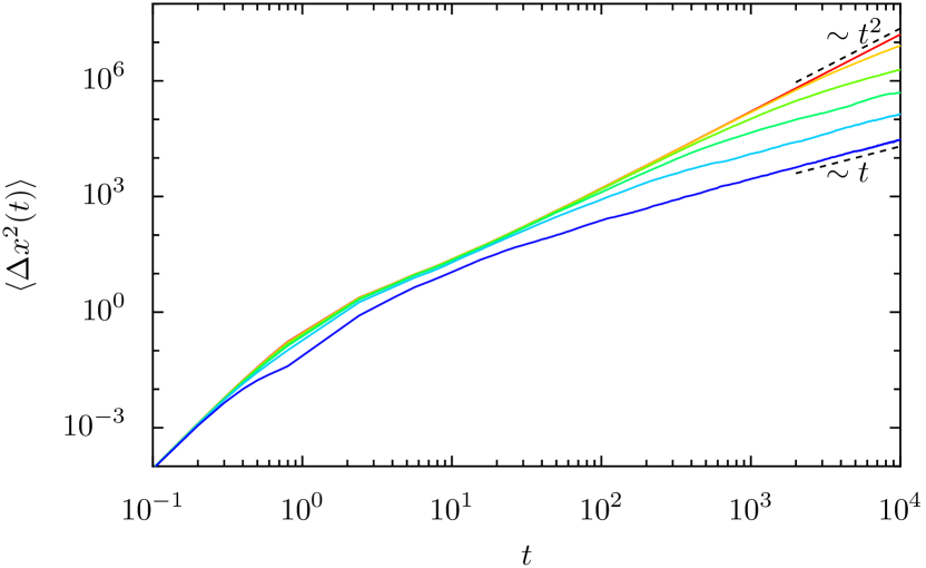
Figure 2: (Color online) Unbiased superdiffusion in a washboard potential. The mean square displacement of a particle that spreads ballistically in the absence of a bias $F$, see Fig. 1, eventually changes its behavior from superdiffusive to normal diffusive behavior under the influence of a periodic potential of strength $V_{0}$. From bottom right hand side to top we use $V_{0}=0.5,0.2,0.1,0.05,0.02,0$. The time of the turn-over shifts to later times with decreasing potential strength. For the simulation of the displayed data the first embedding was used with $\kappa=2$, $\nu=3$, $\omega_{0}=1$ and $v(0)=0$.

III.3 Superdiffusion in a biased washboard potential

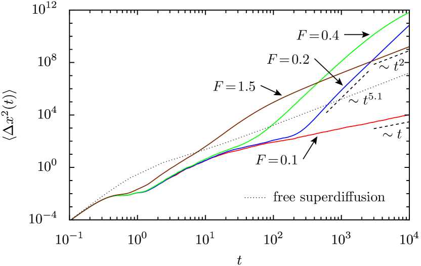
Figure 3: (Color online) Biased superdiffusion. After diffusion has become normal in the presence of a periodic potential, see Fig. 2, it is again changing to ballistic diffusion under the influence of an additional finite bias $F$. Long transients exhibiting hyper-diffusion emerge before the ballistic diffusion regime is approached. A fixed barrier height $V_{0}=1$ was used for the simulations and the tilt $F$ is variable. The other parameters are again $\kappa=2$, $\nu=3$, $\omega_{0}=1$ and $v(0)=0$.

The modification of the dynamics by a tilt of the washboard potential, $V(x,t)=-V_{0}\cos(2\pi x/x_{0})-Fx$, provides an intriguing question. In particular one may ask whether the spreading will again become superdiffusive and whether a supercurrent will emerge that steadily grows with time? The numerical simulations displayed in Figs. 3 and 4 indicate that the answer to both questions is yes. Both the mean square displacement as well as the average displacement become proportional to a ballistic law $t^{2}$. The time at which this presumably asymptotic behavior sets in becomes increasingly larger the smaller the bias force $F$ is. For the stronger forces $F=0.7,1.5$ the ballistic regime has settled within the total time of $t=10^{4}$ which requires a week of computational time on a Pentium PC with 3 GHz tact-frequency. For small forces $F=0.1,0.2$ an approach to a ballistic behavior is not yet visible. We expect it to occur at a later time.

Another interesting feature is the occurrence of very long superdiffusive transient episodes with a mean square displacement growing faster than ballistic as $t^{\alpha_{\text{eff}}}$ with an exponent $\alpha_{\text{eff}}>2$ up to approximately $5$. We call these episodes “hyper-diffusive”. Their occurrence depends on the dimensionless barrier height $V_{0}/k_{B}T$ and the biasing force $F_{0}$. With a larger barrier the total transient time before the asymptotic ballistic behavior sets in becomes larger. For small biasing forces after a short initial period first a regime of normal diffusion is observed which turns over into the hyper-diffusive regime at a time that is the later the smaller the biasing force is. For example, for $V_{0}/k_{B}T=1$ and $F=0.2$ the normal diffusion regime extends approximately over one decade from $t=10$ to $t=100$, and then rapidly turns around $t=2\times 10^{2}$ into hyper-diffusion with $\alpha_{\rm eff}\approx 5.1$, cf. Fig. 3. This behavior continues until the end of the simulation at $t=10^{4}$. Until then the root mean square displacement increases by an amount of $10^{3}-10^{4}$ periods of length $x_{0}$. The turnover to the expected ballistic diffusion can only be observed if the biasing force is larger, but then also the normal diffusion regime disappears.

A similar effect of hyper-diffusive motion was reported by Lü and Bao Lu for a Brownian particle moving in a biased periodic potential under the influence of a super-Ohmic model with a spectral density $J(\omega)\propto\omega^{1.5}$ for $\omega\to 0$. The question whether the hyper-diffusion observed in Ref. Lu is indeed asymptotic or whether it is also a transient phenomenon must still be clarified.

From the different curves displayed in Fig. 3 one can infer that for large times the mean square displacement grows the faster the smaller the biasing forces is, in other words, the ballistic diffusion constant increases with decreasing biasing force and, in particular, is larger than the ballistic diffusion constant of free motion reached for $Fx_{0}\gg V_{0}$. This phenomenon is akin to the effect of giant enhancement of normal diffusion in periodic potentials giant ; giant2 .

The mean displacement $\langle\Delta x(t)\rangle$ exhibits a qualitatively similar behavior as the mean square displacement. After a first transient period whose nature strongly depends on the initial velocity distribution a monotonous growth sets in that changes from linear to quadratic, possibly interrupted by an episode of rapid growth proportional to $t^{\beta}$ with $\beta>2$. cf. Fig. 4. The transitions between the different regimes occur at the same times at which the mean square displacement changes from normal diffusion into the hyper-diffusion and finally to ballistic diffusion. The exponent $\beta$ though is much smaller than the hyper-diffusive exponent $\alpha_{\rm eff}$. This indicates that the transport in this intermediate regime is strongly erratic. While both periods of normal and ballistic diffusion can be characterized by a time-independent Peclet number ${\rm Pe}=x_{0}\langle\Delta x(t)\rangle/\langle\Delta x^{2}(t)\rangle$ Lindner the difference of the exponents $\alpha_{\rm eff}$ and $\beta$ does not allow the definition of a Peclet number in the hyper-diffusive regime. However, both in the normal and the asymptotic ballistic regime a time-independent Peclet number can be defined. For $F=0.1$ the FDT (31) holds with a good accuracy and ${\rm Pe}\approx Fx_{0}/(2k_{B}T)$ in the normal diffusion transport regime, see Figs. 3, 4. Beyond the linear response regime, the FDT (31) is generally violated. Such a wealth of different transport regimes with normal and anomalous features, revealed by a simple model is really surprising.

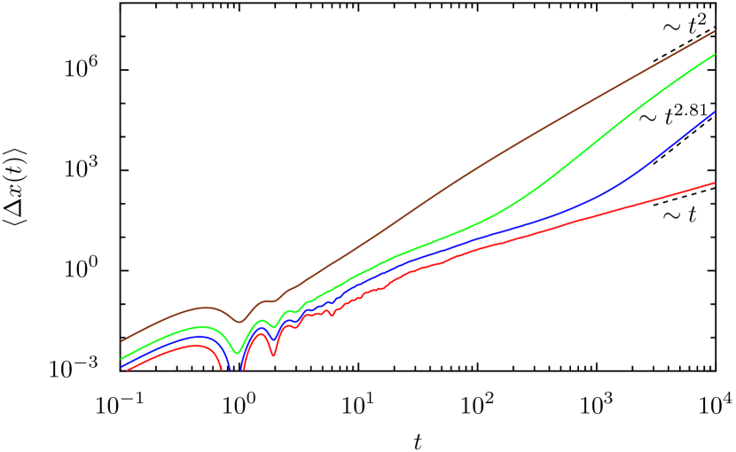
Figure 4: (Color online) Anomalous drift behavior. A finite bias $F$ induces anomalous drift. From bottom right hand side to top we use $F=0.1,0.2,0.4,1.5$. Ballistic currents appear asymptotically $\langle\Delta x(t)\rangle\sim t^{2}$. Like in Fig. 3 transient regimes appear with enhanced particle transport stronger than ballistic. The used parameters are: $V_{0}=1$, $\kappa=2$, $\nu=3$, $\omega_{0}=1$ and $v(0)=0$.

IV Ergodicity

We next comment on the ergodic properties of the velocity fluctuations in relation to ballistic diffusion. In the case of free ballistic diffusion, the velocity fluctuations are clearly non-ergodic. As already mentioned above, this rigorously follows from the fact that the velocity fluctuation correlation coefficient $K_{v}(t)$ given by Eq. (III.1) converges to a constant value different from zero. Also the strong dependence of the position mean square displacement on the initial distribution of the auxiliary variables $u_{1}$ and $u_{2}$ in the limit of large times, see Fig. 1, provides a clear indication of non-ergodicity. In the case of ballistic diffusion in a tilted periodic potential analytic results for the velocity fluctuation autocorrelations are not available and we therefore have to rely on our numerical findings. In Fig. 5 the mean square deviations of position for different distributions of the initial velocities are compared with each other. Apart from minor deviations, these initial preparations do not seem to have any influence in the presence of a tilted periodic potential. Therefore, one might suppose that in this case the process of the velocity fluctuations is wide sense ergodic. This result though cannot be considered conclusive because also in the absence of any potential the choice of the initial distribution of velocities has only little impact on the mean square displacement, see lines labeled by $V_{0}=0,F=0$ in Fig. 5. A more convincing argument results from the comparison of the effect of different initial distributions of the auxiliary variables $u_{1}$ and $u_{2}$, see Fig. 6. While the influence of this distribution on the position mean square deviation is very large and even increases with growing time, see Fig. 1, only small deviations at early and intermediate times are visible in the case of a tilted periodic potential. Hence, numerical evidence seems to indicate that the velocity fluctuations of a ballistically diffusing particle in a tilted washboard potential indeed is wide sense ergodic.

This raises the question whether it is possible that the velocity fluctuations of a superdiffusive process may be wide sense ergodic in one case and non-ergodic in another. The strict answer to this question is that the velocity fluctuations of any truly ballistic diffusion with $\langle\Delta x^{2}(t)\rangle=D_{2}t^{2}$ constitute a non-ergodic process. This follows from Eq. (23) by means of differentiation with respect to time yielding

$$D_{2}=\lim_{t\to\infty}\frac{1}{t}\int_{0}^{t}dt^{\prime}K_{v}(t^{\prime})\;.$$ (36)

Therefore the time average of the autocorrelation function of the velocity fluctuations does not vanish and consequently the velocity fluctuations are non-ergodic, see Appendix B.

However, one must keep in mind that the ballistic diffusion presents a marginal case. Any increase of $\langle\Delta x^{2}(t)\rangle$ slower than $t^{2}$, such as $t^{2-\epsilon}$ with any small, positive $\epsilon$, or $t^{2}/\ln t$ will lead to a vanishing time average of the velocity fluctuation autocorrelation function by the same argument as above. From the numerical point of view there is always a limitation of how accurate the scaling exponent of $\langle\Delta x^{2}(t)\rangle$ can be determined. Logarithmic corrections are almost impossible to identify. We therefore suppose that the observed ballistic diffusion in a tilted washboard potential might strictly speaking be marginally sub-ballistic and the velocity fluctuations wide sense ergodic.

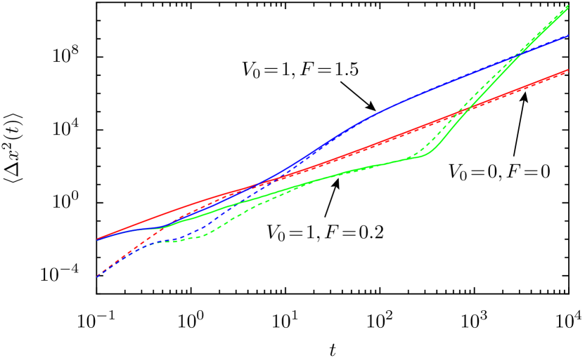
Figure 5: (Color online) Mean square displacement of position for different initially distributed velocities. The solid lines mark thermally distributed initial velocities $\langle v^{2}(0)\rangle=v^{2}_{T}$, whereas dashed lines mark initially zero velocity $v(0)=0$. The differences in time evolution vanish in the asymptotic long time limit in the presence of a biased periodic washboard potential with potential height $V_{0}$ and bias $F$, implying wide sense ergodicity for the mean square displacement. However, in case of free ballistic diffusion, see lines labeled by $V_{0}=0,F=0$, a constant deviation remains according to Eq. (35). Parameters are chosen as $\kappa=2$, $\nu=3$ and $\omega_{0}=1$.

Figure 6: (Color online) Role of deviation from stationary fluctuation-dissipation relation in Eqs. (2, 45) on the time evolution of the mean square displacement $\langle\Delta x^{2}(t)\rangle$. In contrast to the choice with a stationary fluctuation-dissipation relation, see solid lines marking $\langle u_{i}(0)u_{j}(0)\rangle\!=\!\kappa^{2}\delta_{i,j}$, the initial choice $u_{1}(0)\!=\!u_{2}(0)\!=\!0$, see dashed lines, yields a Gaussian noise $\zeta(t)$ that initially is non-stationary, see Eq. (44). The noise $\zeta(t)$ assumes, however, stationary noise at asymptotic long times. The initial velocity was set to zero, i.e. $v(0)=0$, the potential strength to $V_{0}=1$ and the remaining parameters are chosen as in Fig. 5, $\kappa=2$, $\nu=3$ and $\omega_{0}=1$.

V Summary

In this work we considered one of the simplest models for the superdiffusive motion of a particle described by a GLE. It corresponds to a bi-exponential memory kernel with zero integral. The according spectral density $J(\omega)$ of thermal bath oscillators sets in with a cubic law. It describes, for example the diffusion of an impurity in a crystal.

We considered a large family of Markovian embedding schemes, i.e. higher dimensional Markovian processes that generate the considered non-Markovian process upon projection onto the subspace spanned by position and momentum of the particle. Out of the whole class we identified a simple four-dimensional embedding that can be numerically treated in an efficient way.

We confirm that ballistic superdiffusion is non-ergodic, which is concordant with the findings in Bao05 ; Bao05a . As a new amazing manifestation of non-ergodicity we found that a non-equilibrium initial noise preparation can change the law of diffusion, see in Fig. 1.

Further on our numerical findings indicate that the free ballistic diffusion, being present in the absence of any potential, changes into normal diffusion in the presence of a periodic potential. We concluded that the process of the velocity fluctuations is non-ergodic in the absence of a periodic potential but wide sense ergodic in the presence of a periodic potential. Apparently, the transition to the ergodic motion does not require a minimal potential strength. Rather, the time to reach the asymptotic regime of normal diffusion diverges with vanishing potential strength $V_{0}$.

An additional biasing force leads to ballistic motion in a periodic potential, i.e. both the mean value and the variance of the position displacement grow proportional to a $t^{2}$ law. In this case, however we found strong indications that the velocity fluctuations remain wide sense ergodic. This paradoxically looking scenario – non-ergodic for free ballistic diffusion versus ergodic for ballistic diffusion in a potential – is possible because the ballistic diffusion presents a marginal situation. Although for ballistic diffusion following a strict $t^{2}$ law the velocity fluctuations are non-ergodic any modification of the $t^{2}$ law with a weakly decaying function such as $1/\ln t$ leads to wide sense ergodic velocity fluctuations. For a sub-critical bias $F<F_{0}=2\pi V_{0}/x_{0}$ the ballistic diffusion coefficient $D_{2}$ is substantially enhanced compared to the diffusion coefficient for free ballistic diffusion. This effect is the analog to giant enhancement of normal diffusion in tilted washboard potentials.

Depending on the potential and the bias strengths the time before the asymptotic ballistic motion sets in may be extremely large. Within this long transient period a normal and even a hyper-diffusion regime may exist,where $\alpha_{\rm eff}$ exceeds the ballistic value of 2. The presence of such long transients presents a general feature of the studied non-Markovian dynamics.

Acknowledgements This work was supported by the German Excellence Initiative via the Nanosystems Initiative Munich (NIM).

Appendix A Conditions for embedding

The solution of the last equation in Eq. (II) is

$$\roarrow{u}(t)= -\int_{0}^{t}e^{-\mathbf{A}(t-t^{\prime})}p(t^{\prime})\roarrow{r}dt^{\prime}+$$

$$\int_{0}^{t}e^{-\mathbf{A}(t-t^{\prime})}\mathbf{C}\roarrow{\xi}(t^{\prime})dt^{\prime}+e^{-\mathbf{A}t}\roarrow{u}(0)\;,$$ (37)

which inserted into (II) yields

$$\dot{p}(t)= -\left[\frac{\partial}{\partial x}V(x,t)-\roarrow{g}^{\mathrm{T}}\roarrow{u}(t)\right]=$$

$$= -\frac{\partial}{\partial x}V(x,t)-\int_{0}^{t}\roarrow{g}^{\mathrm{T}}e^{-\mathbf{A}(t-t^{\prime})}\roarrow{r}p(t^{\prime})dt^{\prime}+$$

$$\int_{0}^{t}\roarrow{g}^{\mathrm{T}}e^{-\mathbf{A}(t-t^{\prime})}\mathbf{C}\roarrow{\xi}(t^{\prime})dt^{\prime}+\roarrow{g}^{\mathrm{T}}e^{-\mathbf{A}t}\roarrow{u}(0)\;.$$ (38)

The comparison of (A) with (II) gives Eq. (9) and

$$\zeta(t)=\int_{0}^{t}\roarrow{g}^{\mathrm{T}}e^{-\mathbf{A}(t-t^{\prime})}\mathbf{C}\roarrow{\xi}(t^{\prime})dt^{\prime}+\roarrow{g}^{\mathrm{T}}e^{-\mathbf{A}t}\roarrow{u}(0)\;.$$ (39)

Assuming $\langle u_{i}(0)\xi_{j}(t)\rangle=0$, this enables one to calculate the noise correlation function:

$$\langle\zeta(t)\zeta(s)\rangle=\langle\roarrow{g}^{\mathrm{T}}e^{-\mathbf{A}t}\roarrow{u}(0)\roarrow{g}^{\mathrm{T}}e^{-\mathbf{A}s}\roarrow{u}(0)\rangle$$

$$+\langle\int_{0}^{t}dt^{\prime}\int_{0}^{s}ds^{\prime}\roarrow{g}^{\mathrm{T}}e^{-\mathbf{A}(t-t^{\prime})}\mathbf{C}\roarrow{\xi}(t^{\prime})\roarrow{g}^{\mathrm{T}}e^{-\mathbf{A}(s-s^{\prime})}\mathbf{C}\roarrow{\xi}(s^{\prime})\rangle$$ (40)

Taking into account Eq. (8) for $t>s$ (the case $t<s$ can be treated alike) the second term reduces to:

$$\int_{0}^{s}\roarrow{g}^{\mathrm{T}}e^{-\mathbf{A}(t-s^{\prime})}\mathbf{C}\mathbf{C}^{\mathrm{T}}e^{-\mathbf{A}^{\mathrm{T}}(s-s^{\prime})}\roarrow{g}ds^{\prime}=$$

$$=\roarrow{g}^{\mathrm{T}}e^{-\mathbf{A}t}\int_{0}^{s}e^{\mathbf{A}s^{\prime}}\mathbf{C}\mathbf{C}^{\mathrm{T}}e^{\mathbf{A}^{\mathrm{T}}s^{\prime}}ds^{\prime}e^{-\mathbf{A}^{\mathrm{T}}s}\roarrow{g}$$ (41)

and the first term is:

$$\langle\!\roarrow{g}^{\mathrm{T}}e^{-\mathbf{A}t}\roarrow{u}(0)\roarrow{g}^{\mathrm{T}}e^{-\mathbf{A}s}\roarrow{u}(0)\!\rangle=$$

$$= \roarrow{g}^{\mathrm{T}}e^{-\mathbf{A}t}\langle\!\roarrow{u}(0)\otimes\roarrow{u}^{\mathrm{T}}(0)\!\rangle e^{-\mathbf{A}^{\mathrm{T}}s}\roarrow{g}\;.$$ (42)

Altogether, with the following definition:

$$\mathbf{U}\equiv\langle\!\roarrow{u}(0)\otimes\roarrow{u}^{\mathrm{T}}(0)\!\rangle$$ (43)

this yields:

$$\langle\!\zeta(t)\zeta(s)\!\rangle=\roarrow{g}^{\mathrm{T}}e^{-\mathbf{A}t}\left[\mathbf{U}+\int_{0}^{s}e^{\mathbf{A}s^{\prime}}\mathbf{C}\mathbf{C}^{\mathrm{T}}e^{\mathbf{A}^{\mathrm{T}}s^{\prime}}ds^{\prime}\right]e^{-\mathbf{A}^{\mathrm{T}}s}\roarrow{g}\;.$$

Making an Ansatz as in Eq.(11) enables one to separate the noise correlation function into a stationary and a non-stationary part:

$$\langle\!\zeta(t)\zeta(s)\!\rangle= \roarrow{g}^{\mathrm{T}}e^{-\mathbf{A}t}\left[\mathbf{U}+\int_{0}^{s}e^{\mathbf{A}s^{\prime}}(\mathbf{A}\mathbf{G}+\mathbf{G}\mathbf{A}^{\mathrm{T}})e^{\mathbf{A}^{\mathrm{T}}s^{\prime}}ds^{\prime}\right]$$

$$\times e^{-\mathbf{A}^{\mathrm{T}}s}\roarrow{g}=$$

$$= \roarrow{g}^{\mathrm{T}}e^{-\mathbf{A}t}\left[\mathbf{U}+e^{\mathbf{A}s^{\prime}}\mathbf{G}e^{\mathbf{A}^{\mathrm{T}}s^{\prime}}\Big{|}_{s^{\prime}=0}^{s^{\prime}=s}\right]e^{-\mathbf{A}^{\mathrm{T}}s}\roarrow{g}=$$

$$= \roarrow{g}^{\mathrm{T}}e^{-\mathbf{A}t}\left[\mathbf{U}-\mathbf{G}\right]e^{-\mathbf{A}^{\mathrm{T}}s}\roarrow{g}+\roarrow{g}^{\mathrm{T}}e^{-\mathbf{A}(t-s)}\mathbf{G}\roarrow{g}$$ (44)

The first term of Eq. (44) represents the non-stationary part and is vanishing asymptotically in the limit of long times, i.e. $t,s\to\infty$. Both the relaxation spectrum defining the corresponding time scales and the spectrum of autocorrelation times is given by the eigenvalues of matrix $\mathbf{A}$. Moreover, the fluctuation-dissipation relation of Eq. (2) is always asymptotically fulfilled, if one chooses $\mathbf{G}\roarrow{g}=mk_{B}T\roarrow{r}$, which yields Eq. (10). However, in order to obey the fluctuation-dissipation relation for all times, one has to set $\mathbf{U}\equiv\mathbf{G}$, which implies Eq. (12) and we end with:

$$\langle\!\zeta(t)\zeta(s)\!\rangle=mk_{B}T\roarrow{g}^{\mathrm{T}}e^{-\mathbf{A}(t-s)}\roarrow{r}=mk_{B}T\gamma(t-s)\;.$$ (45)

Appendix B Wide sense ergodicity

According to its definition, a stationary process $y(t)$ is ergodic in the wide sense if its time average converges in the mean square sense towards the ensemble average. This definition implies that a process $y(t)$ is wide sense ergodic if and only if the time average of the autocorrelation function of its fluctuations vanishes, i.e. if

$$\lim_{t\to\infty}\frac{1}{t}\int_{0}^{t}dt^{\prime}\langle(y(t)-\langle y\rangle)(y(0)-\langle y\rangle)\rangle=0$$ (46)

holds Yaglom . Hence, the decay of the autocorrelation function of the fluctuations towards zero provides a sufficient condition for a wide sense ergodic process. On the other hand, the considered process is non-ergodic if the autocorrelation function of its fluctuations approaches a constant value different from zero.

References

- (1) H. Scher, E.W. Montroll, Phys. Rev. B 12, 2455 (1975).
- (2) M. Shlesinger, J. Stat. Phys. 10, 421 (1974).
- (3) B. D. Hughes, Random Walks and Random Environments (Clarendon Press, Oxford, 1995).
- (4) J. P. Bouchaud and A. Georges, Phys. Rep. 195, 127 (1990).
- (5) R. Metzler, J. Klafter, Phys. Rep. 339, 1 (2000).
- (6) R. Metzler, E. Barkai, and J. Klafter, Phys. Rev. Lett. 82, 3563 (1999).
- (7) H. C. Fogedby, Phys. Rev. E 50, 1657 (1994).
- (8) A. A. Stanislavsky, Phys. Rev. E 67, 021111 (2003).
- (9) P. D. Ditlevsen, Phys. Rev. E 60, 172 (1999).
- (10) A. Dubkov and B. Spagnolo, Fluct. Noise Lett. 5, L267 (2005).
- (11) S. Marksteiner, K. Ellinger, and P. Zoller, Phys. Rev. A 53, 3409 (1996).
- (12) E. Lutz, Phys. Rev. Lett. 93, 190602 (2004).
- (13) E. Barkai and R. J. Silbey, J. Phys. Chem. B 104, 3866 (2000).
- (14) R. Friedrich, F. Jenko, A. Baule, and S. Eule, Phys. Rev. Lett. 96, 230601 (2006).
- (15) K. G. Wang and M. Tokuyama, Physica A 265, 341 (1999).
- (16) R. Morgado, F. A. Oliveira, G. G. Batrouni, A. Hansen, Phys. Rev. Lett. 89, 100601 (2002).
- (17) N. Pottier, Physica A 317, 371 (2003).
- (18) U. Weiss, Quantum Dissipative Systems, 2nd ed. (World Scientific, Singapore, 1999).
- (19) R. Kubo, Rep. Prog. Phys. 29, 255 (1966).
- (20) N. N. Bogolyubov, in: On some Statistical Methods in Mathematical Physics (Acad. Sci. Ukrainian SSR, Kiev, 1945), 115-137, in Russian.
- (21) R. Zwanzig, J. Stat. Phys. 9, 215 (1973).
- (22) P. Hänggi, P. Talkner, and M. Borcovec, Rev. Mod. Phys. 62, 251 (1990).
- (23) J.-D. Bao, J. Stat. Phys. 114, 503 (2004).
- (24) J.-D. Bao, Y.-Z. Zhuo, F. A. Oliveira, and P. Hänggi, Phys. Rev. E 74, 061111 (2006).
- (25) J.-D. Bao, Y.-L. Song, Q. Ji, and Y.-Z. Zhuo, Phys. Rev. E 72, 011113 (2005).
- (26) J.-D. Bao, P. Hänggi, Y.-Z. Zhuo, Phys. Rev. E 72, 061107 (2005).
- (27) S. A. Adelman, J. Chem. Phys. 64, 124 (1976).
- (28) P. Hänggi and H. Thomas, Z. Physik B 26, 85 (1977).
- (29) P. Hänggi, H. Thomas, H. Grabert, and P. Talkner, J. Stat. Phys. 18, 155 (1978).
- (30) P. Hänggi, Z. Physik B 31, 407 (1978).
- (31) P. Hänggi and F. Mojtabai, Phys. Rev. A 26, 1168 (1982).
- (32) If the matrix can only be brought into Jordan normal form, will have less than exponentials and additional terms of the form .
- (33) F. Marchesoni and P. Grigolini, J. Chem. Phys. 78, 6287 (1983).
- (34) R. Kupferman, J. Stat. Phys. 114, 291 (2004).
- (35) I. Goychuk, Phys. Rev. E 80, 046125 (2009).
- (36) T. C. Gard, Introduction to Stochastic Differential Equations (Dekker, New York, 1988).
- (37) W. H. Press, S. A. Teukolsky, W. T. Vetterling, B. P. Flannery, Numerical Recipes: The Art of Scientific Computing, 3d ed. (Cambridge University Press, Cambridge, 2007).
- (38) W. Deng and E. Barkai, Phys. Rev. E 79, 011112 (2009).
- (39) A. Papoulis, Probability, Random Variables, and Stochastic Processes (McGraw-Hill Book Company, New York, 1965); see Sect. 9-8, pp. 323-335.
- (40) K. Lü, and J.-D. Bao, Phys. Rev. E 76, 061119 (2007).
- (41) B. Lindner, M. Kostur, and L. Schimansky-Geier, Fluct. Noise Lett. 1, R25 (2001).
- (42) P. Reimann, C. Van den Broeck, H. Linke, P. Hänggi, J. M. Rubi, and A. Perez-Madrid, Phys. Rev. Lett. 87, 010602 (2001).
- (43) P. Reimann, C. Van den Broeck, H. Linke, P. Hänggi, J. M. Rubi, and A. Perez-Madrid, Phys. Rev. E 65, 031104 (2002).
- (44) A.M. Yaglom, An Introduction to the Theory of Stationay Random Functions, Dover Publications, New York, 1972; see Sect. 1.4.