Resonance Scattering in Optical Lattices and Molecules:
Interband versus Intraband Effects

Abstract

We study the low-energy two-body scattering in optical lattices with higher-band effects included in an effective potential, using a renormalization group approach. The approach captures most dominating higher band effects as well as all multiple scattering processes in the lowest band. For an arbitrary negative free space scattering length($a_{s}$), a resonance of low energy scattering occurs as lattice potential depths reaches a critical value $v_{c}$; these resonances, with continuously tunable positions $v_{c}$ and widths $W$, can be mainly driven either by intraband or both intra- and interband effects depending on the magnitude of $a_{s}$. We have also studied scattering amplitudes and formation of molecules when interband effects are dominating, and discussed an intimate relation between molecules for negative $a_{s}$ and repulsively bound states pioneered by Winkler et al.Winkler06 .

For a dilute ultracold atomic gas, the two-body s-wave scattering length $a_{s}$ is known to be conveniently tunable via magnetic-field-induced Feshbach resonancestheory ; expe . Experimentally in the presence of external trapping confinements, however, binary atomic collision properties can be dramatically modified as revealed both theoretically and experimentally in three-dimensional (3D) harmonic trapsBusch98 ; Stoferle06 ; Ospelkaus06 , and in waveguidesOlshanii ; Pricoupenko08 ; Moritz05 ; Petrov . Remarkably, the waveguide confinement can result in very peculiar effective potentials as pointed out in a few early papersOlshanii ; Petrov ; especially, Olshanii et al. systematically studied scattering between atoms in a 1D waveguide and found that the effective potential for atoms in the lowest transverse mode can reach the hardcore limit. Interacting atoms in optical lattices are another subject that has attracted enormous interests for the past few yearsBloch02 ; Esslinger05 ; Ketterle06 . However, till now what happens to binary collisions in an optical lattice on the other hand have not been thoroughly studied and the subject of molecules of Bloch waves is also not well understood. It is becoming essential to understand the fundamentals of two-body scattering and other few-body physics of Bloch states; such analyses should form building blocks for future many-body theories and set potential references for quantitative calculations of parameters in many-body Hamiltonians. Studies of this issue can further cast light on dynamics of colliding atoms or condensates in optical lattices and coherent control of atoms in optical latticesBloch03 .

Low energy scattering in an optical lattice was previously investigated and resonance scattering was pointed out for attractive interactionsFedichev04 . Studies there were carried out in an approximation where laser potentials are approximated as harmonic ones so that the center-of-mass motion is decoupled from the relative motion of two scattering atoms; effectively the problem was reduced to two-body scattering within an individual lattice site, which is justifiable for deep lattices. In this Letter to reveal how Bloch waves are scattered in optical lattices at different depths, we propose an approach to resonance scattering without utilizing the approximations of separable potentials in Ref.Fedichev04 . Our approach captures most dominating higher band effects as well as all intraband scattering within the lowest band. It is valid for studies of resonances in deep lattices at small $a_{s}$ as well as resonances in shallow ones at large $a_{s}$. And when applying our approach to lower dimensional waveguides, we obtain identical results discussed previously Olshanii ; Petrov .

Our main proposal is to evaluate $U_{eff}$, the effective potential for atoms in the lowest band that takes into account multiple virtual scattering processes involving higher bands, and then apply the same procedure to calculate the full $T$-matrix of low-energy scattering. When free space scattering lengths $|a_{s}|$ are comparable to or larger than the lattice constant $a_{L}$, virtual scattering to higher bands contributes substantially to scattering in the lowest band and resonance scattering is driven by both interband and intraband effects. We find that the higher-band effects on physical quantities are most pronounced in shallow lattices near resonances(see Fig.3,4). When magnitudes of $a_{s}$ are arbitrarily small, resonance scattering at the bottom of the lowest band is predominately driven by intraband virtual scattering and is induced mainly by the enhanced effective masses of atoms in optical lattices.

To facilitate discussions on low-energy scattering atoms, we start with a two-body Hamiltonian

$$H=\sum_{\alpha}\epsilon_{\alpha}|\alpha\rangle\langle\alpha|+\sum_{\alpha\beta}U_{\alpha\beta}|\alpha\rangle\langle\beta|,$$ (1)

with $|\alpha(\beta)\rangle$ being arbitrary two-body scattering states. For scattering in free space with a short range potential approximated as $U(\mathbf{r})=U_{0}\delta^{3}(\mathbf{r})$, $|\alpha\rangle,|\beta\rangle=|{\bf k},-{\bf k}\rangle$ and $U_{\alpha\beta}=\frac{U_{0}}{\Omega}$ with $\Omega$ the volume; to obtain an effective low-energy Hamiltonian, we employ the momentum-shell renormalization group(RG) equation approachKaplan98 . The key idea here is at an arbitrary cutoff momentum $\Lambda$, we can further divide the ${\bf k}$-space into two regions, i.e., a core region defined by $|{\bf k}|<\Lambda-\delta\Lambda$ and a shell $\Lambda-\delta\Lambda<|{\bf k}|<\Lambda$. Correspondingly, we split the Hamiltonian at a given cutoff $\Lambda$ into three pieces $H(\Lambda)=H^{<}+H^{>}+H^{><}$ which respectively describe interacting atoms within the core, within the shell and the scattering in between. For atoms with $|{\bf k}|\ll\Lambda$, the second-order virtual scattering into high energy states within the shell caused by $H^{><}$ modifies the low-energy scattering amplitudes and results in a correction $(\delta U)$ in $H^{<}$. One can then obtain a differential RG equation for effective potential $U(\Lambda)$ in $H(\Lambda)$ in terms of the cutoff $\Lambda$,

$$\frac{1}{U^{2}}\frac{\delta U}{\delta\Lambda}=\frac{1}{\Omega}\frac{\delta}{\delta\Lambda}(\sum_{|{\bf k}|<\Lambda}\frac{1}{2\epsilon_{\bf k}}).$$ (2)

So the effective potential $U$ for scattering atoms at momenta smaller than ${\Lambda}$ is renormalized due to the coupling to virtual states at larger momenta and is given as

$$\frac{1}{U(\Lambda)}=\frac{1}{U(\Lambda^{*})}+\frac{1}{\Omega}\sum_{\Lambda<|{\bf k}|<\Lambda^{*}}\frac{1}{2\epsilon_{\bf k}}.$$ (3)

Boundary conditions $U(\Lambda^{*})=U_{0}$ and $U(0)=T_{0}$ relate $U_{0}$ to the low-energy scattering length $a_{s}(=\frac{mT_{0}}{4\pi})$ via $\frac{m}{4\pi a_{s}}=\frac{1}{U_{0}}+\frac{1}{\Omega}\sum_{|\mathbf{k}|<\Lambda^{*}}\frac{1}{2\epsilon_{\mathbf{k}}}$. ($\Lambda^{*}$ is an ultraviolet momentum cut-off that is set by the range of interactions.)

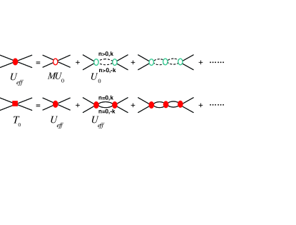
Figure 1: (color online). Virtual scattering processes that contribute to scattering potential $T_{0}$ in optical lattices. Different two-particle vertex functions are indicated below the diagrams. Solid (dashed) lines between two vertices represent states in the lowest $n=0$ band (higher $n>0$ bands).

One can apply a similar idea to optical lattices. For a cubic optical lattice with potential $V(\mathbf{r})=V_{0}\sum_{i=x,y,z}\sin^{2}(\frac{2\pi x_{i}}{\lambda})$ and spacing $a_{L}=\frac{\lambda}{2}$, Bloch states $\phi_{n\mathbf{k}}(\mathbf{r})=\frac{1}{\sqrt{\Omega}}\sum_{\mathbf{G}}w_{n}(\mathbf{k+G})e^{i(\mathbf{k}+\mathbf{G})\cdot\mathbf{r}}$ and energies $\epsilon_{n\mathbf{k}}$ can be numerically obtained; here $n$ are band indices; $\mathbf{k}\in BZ$(Brillouin zone) is a quasi-momentum and $\mathbf{G}$ (and $\mathbf{Q}$ below) are the reciprocal lattice vectors; eigenvector $w_{n}(\mathbf{q})$ is the Wannier wavefunction in momentum space. We specify potential depth $V_{0}$ in units of the recoil energy $E_{R}=\frac{\pi^{2}}{2ma_{L}^{2}}$ via a dimensionless quantity $v=\frac{V_{0}}{E_{R}}$.

First we calculate the interaction matrix element between Bloch states $|\alpha\rangle=|\{m,\mathbf{k}\},\{n,-\mathbf{k}\}\rangle$ and $|\beta\rangle=|\{m^{\prime},\mathbf{k^{\prime}}\},\{n^{\prime},-\mathbf{k^{\prime}}\}\rangle$,

$$U_{\alpha\beta} \equiv \langle\alpha|U|\beta\rangle=\frac{U_{0}}{\Omega}\sum_{\mathbf{Q}}M_{\alpha}^{\mathbf{Q}\ *}M_{\beta}^{\mathbf{Q}},$$ (4)

here $M_{\alpha}^{\mathbf{Q}}=\sum_{\mathbf{G}}w_{m}(\mathbf{k+G})w_{n}(\mathbf{Q-k-G})$. Relevant matrix elements of $U_{\alpha\beta}$ can be classified into three categories: A) $|\{0,{\bf k}\};\{0,-{\bf k}\}\rangle\leftrightarrow|\{0,{\bf k}^{\prime}\};\{0,-{\bf k}^{\prime}\}\rangle$, i.e. scattering within the lowest band, $U_{\alpha\beta}$ are given as $MU_{0}$M ; these represent the most dominating processes; B) $|\{n,{\bf k}\};\{n,-{\bf k}\}\rangle\leftrightarrow|\{n^{\prime},{\bf k}^{\prime}\};\{n^{\prime},-{\bf k}^{\prime}\}\rangle$ with $n\neq 0$ or $n^{\prime}\neq 0$ which constitute the most important scattering processes involving higher bands, give the next dominating contributions that are approximately equal to $U_{0}$ (deviations are typically of order of $\frac{v^{2}}{32}$ or less in shallow lattices); C) $|\{n,{\bf k}\};\{n,-{\bf k}\}\rangle\leftrightarrow|\{m^{\prime},{\bf k}^{\prime}\};\{n^{\prime},-{\bf k}^{\prime}\}\rangle$ with $m^{\prime}\neq n^{\prime}$, i.e. scattering involving two atoms in different bands; they contribute the least in shallow lattices (of order of $\frac{v}{8}$ or less) because of the approximate translational symmetry.

In shallow lattices at an arbitrary $a_{s}$, we can always neglect matrix elements in C-class and only keep those in A- and B-class. In deep lattices near resonances where $a_{s}$ are small, we keep matrix elements in B-class to remove the ultraviolet divergence when summing up the virtual scattering to high energy states; the residue higher band effects after regularization turn out to be negligible and we again neglect C-class scattering processes; and our treatments of scattering processes within the lowest band become exact in this limit. However, for large $a_{s}$ and deep lattices that are away from the resonances, contributions from C-class scattering can be comparable to other classes; and by neglecting C-class contributions, we obtain in this limit estimates only good for qualitative understanding. To study resonances, below we adopt a simplest two-coupling-constant model(See Fig.1) which yields reasonable estimates of higher band effects.

Using the general features of $U_{\alpha\beta}$ discussed above and following the idea outlined before Eq.(3), we obtain the effective potential $U_{eff}$ for the lowest band and further calculate the scattering potential $T_{0}$ for states near $\epsilon_{n\mathbf{k}}=0$, as diagrammatically shown in Fig.1, to be

$$\frac{1}{U_{eff}} = \frac{m\eta}{4\pi a_{L}M}(\frac{a_{L}}{a_{s}}-C_{1}),$$

$$\frac{1}{T_{0}} = \frac{m\eta}{4\pi a_{L}M}(\frac{a_{L}}{a_{s}}-C_{1}+C_{2}),$$ (5)

with $C_{1,2}$ defined as

$$C_{1} = \frac{4\pi a_{L}}{m\Omega}\big{(}\sum_{\mathbf{k}}\frac{1}{2\epsilon_{\mathbf{k}}}-\sum_{n>0,\mathbf{k}}\frac{1}{2\epsilon_{n\mathbf{k}}}\big{)},$$

$$C_{2} = \frac{4\pi a_{L}}{m\eta\Omega}\sum_{n=0,\mathbf{k}}\frac{M}{2\epsilon_{n\mathbf{k}}}.$$ (6)

Here $\eta=(1+(1-\frac{1}{M})\frac{U_{0}}{\Omega}\sum_{n>0,\mathbf{k}}\frac{1}{2\epsilon_{n\mathbf{k}}})^{-1}$ is close to unity in the regions that interest useta ; evidently $C_{1}$ and $C_{2}$ are respectively ascribed to interband and intraband scattering effects. Note that when $a_{s}$ is much bigger than $a_{L}$, $U_{eff}$ saturates at a value of $-4\pi a_{L}M/mC_{1}$.

Figure 2: (a)Interband($C_{1}$) and intraband($C_{2}$) effects vs lattice potentials $v$. Inset shows the ratio. (b)Resonance position $v_{c}$ vs $a_{L}/a_{s}$; dashed line is $v_{c}$ calculated without interband contributions (i.e. $C_{1}=0$.) (c)Width $W(v_{c})$. Solid and dashed lines are fit to $\frac{2}{v_{c}}$ and $\frac{4}{\pi\gamma}\sqrt{v_{c}}$ respectively.

Our results of $C_{1,2}$ are shown in Fig.2. At $v=0$ and $M=1$, we reproduce the free space result $T_{0}=4\pi a_{s}/m$. With increasing $v$, the intraband scattering gradually takes a dominating role over other ones, reflected by a much more rapid increase of $C_{2}$ than $C_{1}$. For instance at $v=5$, $C_{1}/C_{2}=0.21$. In the large-$v$ limit, with the lowest band spectrum $\epsilon_{\mathbf{k}}=t\sum_{i}(1-\cos{k_{i}a_{L}})$, $t$ being the hopping amplitude, we find that

$$C_{1}=\sqrt{8}v^{\frac{1}{4}},\ C_{2}=\frac{\pi\gamma}{32\sqrt{2}}e^{2\sqrt{v}}\ (\gamma\approx 4).$$ (7)

To obtain Bloch wave scattering length $a_{bloch}$ we first introduce an effective(band) mass $m_{eff}=1/\frac{\partial^{2}\epsilon_{nk}}{\partial k^{2}}|_{0}$ and relate it to the scattering potential $T_{0}=4\pi a_{bloch}/m_{eff}$. For a negative $a_{s}$, a resonance ($a_{bloch}\rightarrow\infty$) occurs at lattice potential $v_{c}$ when $\frac{a_{L}}{a_{s}}=-(C_{2}-C_{1})$. Across the resonance, $a_{bloch}$ obeys an asymptotic equation

$$\frac{a_{bloch}}{a_{L}}=\frac{W(v_{c})}{v-v_{c}}.$$ (8)

In the limit of $|a_{s}|\ll a_{L}$, $v_{c}$ and $W$ can be estimated using Eq.(7); in the opposite limit, they can be obtained using the perturbation theory with respect to $v$,

$$|a_{s}|\ll a_{L} : \ \ v_{c}=\frac{1}{4}\ln^{2}(\frac{32\sqrt{2}}{\pi\gamma}\frac{a_{L}}{|a_{s}|}),\ W=\frac{4}{\pi\gamma}\sqrt{v_{c}};$$

$$|a_{s}|\gg a_{L} : \ \ v_{c}=2\sqrt{\frac{a_{L}}{|a_{s}|}},\ W=\frac{2}{v_{c}}.$$

Both $v_{c}$ and $W$ are continuously tunable by varying $a_{s}$. For ultracold isotopes with negative zero-field scattering lengths such as ${}^{85}Rb|2,2\rangle$ $(-390a_{0})$, ${}^{39}K|1,1\rangle$ $(-45a_{0})$ and ${}^{7}Li|2,2\rangle$ $(-27a_{0})$, using parameters in Bloch09 we find resonances at $v_{c}=5.5,10.0,11.7$ respectively; for ${}^{87}Rb$ and ${}^{40}K$ atoms with interspecies scattering length $a_{bf}=-177a_{0}$, resonance scattering occurs at $v_{c}=7.1$.

For very small $|a_{s}|$, $|a_{s}|\ll\frac{a_{L}}{C_{1}}$, the effective potential $U_{eff}$ can be simply related to the on-site interaction $U_{H}$ in the Hubbard model, $\frac{U_{eff}}{\Omega}=\frac{U_{H}}{N_{L}}$ ($\Omega=N_{L}a_{L}^{3}$). Following Eq.(5-8), we express $a_{bloch}$ as

$$\frac{a_{bloch}}{a_{L}}=\frac{1}{4\pi}(\frac{t}{U_{H}}+\frac{\gamma}{16})^{-1},$$ (9)

which predicts a resonance at $\frac{t}{U_{H}}\approx-0.25$.

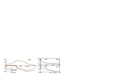
Figure 3: (color online). (a) Real($f_{R}$) and imaginary($f_{I}$) components of $f({E})=\frac{4\pi a_{L}}{m}(T^{-1}(E)-T_{0}^{-1})$ in an optical lattice with depth $v=2.5$ (the band width $6t=1.55E_{R}$). $f_{I}$ is related to the normalized density of state $\rho(\epsilon)$, ${f_{I}=4\rho(\frac{E}{2E_{R}})}$. $f(E)$ calculated without interband effects ($C_{1}=0$) or using a Hubbard (Hub) model are also shown. (b,c) Scattering cross sections($4\pi a^{2}_{L}|\chi|^{2}$, near the bottom of the band) and phase shifts($\theta$) at $a_{s}=-0.5a_{L}$ (resonance position $v_{c}=2.37$) and $v=2.5$, calculated using T-matrix, $|\chi|e^{i\theta}=\frac{m_{eff}T(E)}{4\pi a_{L}}$. Dashed lines are the data without interband effects.

We now turn to scattering matrix $T(E)$ for two atoms with total energy $E$Messiah . Using identical diagrams as shown in Fig.1, one can introduce a Lippmann-Schwinger equation for two scattering atoms in optical lattices; the solutions for $T(E)$ can be obtained as

$$\frac{1}{{T(E)}} = \frac{m\eta(E)}{4\pi a_{L}M}(\frac{a_{L}}{a_{s}}-C_{1}(E)+C_{2}(E)),$$ (10)

where $C_{1,2}(E)$ can be obtained by substituting $\epsilon_{n\mathbf{k}}$ in $C_{1,2}$ of Eq.(5),(6) with $\epsilon_{n\mathbf{k}}-E/2-i0^{+}$. At small $E$, the first two terms in the bracket in Eq.(10) can be approximated to be $U_{eff}$ that dictates the low energy scattering. Fig.3 shows cross sections and phase shifts in shallow lattices where higher band effects are dominating (See (b),(c)). When $E$ is approaching zero, asymptotically we have $T^{-1}(E)=\frac{m_{eff}}{4\pi}(a^{-1}_{bloch}+\beta k^{2}_{E}a_{L}+ik_{E}),\ k_{E}=\sqrt{m_{{}_{eff}}E}$ and $\beta$ approaches $0.03\pi$ when $C_{1}$ is negligible. T-matrix and scattering phase shifts in optical lattices exhibit much richer $E$-dependence than in free space; this is mainly due to a relatively large range of effective interactions (of order of $a_{L}$) in the lowest band compared to that of free space resonances, or a small resonance energy width (of order of $t$ as suggested in Eq.(9)).

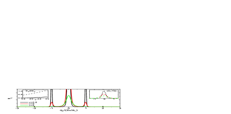
Figure 4: (color online). Real momentum distribution $n_{\mathbf{q}}$($q_{x}=q_{y}=0$, normalized) of bound states at different potential depths $v(>v_{c})$; $a_{s}=-0.5a_{L}$ and the resonance occurs at $v_{c}=2.37$. Right inset shows results without higher band effects(i.e. $C_{1}=0$) and the left one shows the binding energy (dashed line is the estimate without $C_{1}$); note that neglecting higher band effects severely overestimates $|E_{B}|$ leading to a much less singular momentum distribution function $n_{\mathbf{q}}$.

Beyond $v_{c}$, a stable molecule can be formed with a binding energy $E_{B}(<0)$. $E_{B}$ can be obtained by solving the following two-body equation

$$0 = \frac{m\eta}{4\pi a_{L}M}(\frac{a_{L}}{a_{s}}-C_{1}(E_{B})+C_{2}(E_{B})),$$ (11)

Near resonances, $|E_{B}|$ is proportional to $a_{bloch}^{-2}$ (see Eq.(8) for $a_{bloch}$) with the same scaling dimension as in free space. For a bound state $|\Psi\rangle=\sum_{n\mathbf{k}}c_{n\mathbf{k}}\psi^{{\dagger}}_{n\mathbf{k}}\psi^{{\dagger}}_{\mathbf{n-k}}$ , $n_{\mathbf{q}}=\sum_{n\mathbf{kG}}\delta_{\mathbf{q,k+G}}\ |w_{n}(\mathbf{k+G})|^{2}|c_{n\mathbf{k}}|^{2}$ and $c_{n\mathbf{k}}$ is proportional to $1/(2\epsilon_{n\mathbf{k}}-E_{B})$. In Fig.4, we plot $n_{\mathbf{q}}$ for $a_{s}=-0.5a_{L}$ where higher band effects are dominating.

In the limit of deep latticesWinkler06 ; Wouters06 , one can neglect higher band effects by setting $C_{1}(E)=0$ in Eq.(10),(11) and $\eta(E)=1$. Both the T-matrix and the binding energy in this limit exhibit a generalized particle-hole symmetry due to a property of the single particle density of states, $\rho({\epsilon})=\rho(6t-\epsilon)$. So for a given scattering length $a_{s}$, one finds that $ReT^{-1}(E)+ReT^{-1}(12t-E)=ReT^{-1}(12t)+ReT^{-1}(0)$ and $ImT^{-1}(E)=ImT^{-1}(12t-E)$(see Fig.3a). More important, the stable molecules below the lowest band for negative scattering lengths $a_{s}(<0)$ have close connections to mid-gap repulsively bound states for positive scattering lengths that were first thoughtfully pointed out by Winkler et al.Winkler06 . In addition, the T-matrix for negative $a_{s}$ can also be related to that for positive $a_{s}$ via a simple reflection symmetry. Indeed, by examining Eq.(10), (11) in the limit of deep lattices we verify the following exact relations between $a_{s}(<0)$ and $-a_{s}(>0)$ cases, $T(E,a_{s})=-T^{*}(12t-E,-a_{s})$, $-E_{B}(a_{s})=E_{B}(-a_{s})-12t$; resonance scattering and bound states near the bottom of lowest band for a negative $a_{s}$ therefore imply resonance scattering and bound states near the the top of the band for a positive scattering length $-a_{s}$. Note that our equation for the repulsively bound states in this particular limit is identical to the one in Ref.Winkler06 .

In conclusion, we have developed an approach to low-energy resonance scattering in optical lattices taking into account not only the intraband physics but more importantly higher band effects. The resonance scattering in optical lattices offers an alternative path to unitary cold Bose gases so far mainly studied via Feshbach resonancesJin08 . Resonances can also be utilized to study exciting few-body physics of heteronuclear moleculesPetrov07 and Efimov states. We thank Immanuel Bloch, Hanspeter Büchler, Gora Shlyapnikov, Victor Gurarie, Maxim Olshanii, Dmitry Petrov, Leo Radzihovsky and Ruquan Wang for stimulating discussions and the KITPc 2009 cold atom workshop in Beijing for its hospitality. This work is in part supported by NSFC, $973$-Project (China), and by NSERC (Canada), Canadian Institute for Advanced Research.

References

- (1) E. Tiesinga et al., Phys. Rev. A 47, 4114 (1993); J. P. Burke et al., Phys. Rev. Lett. 81, 3355 (1998).
- (2) S. Inouye et al., Nature 392, 151 (1998); Ph. Courteille et al., Phys. Rev. Lett. 81, 69 (1998); J. L. Roberts et al., Phys. Rev. Lett. 81, 5109 (1998).
- (3) T. Busch et al., Found. Phys. 28, 549 (1998).
- (4) T. Stöferle et al., Phys. Rev. Lett. 96, 030401 (2006).
- (5) C. Ospelkaus et al., Phys. Rev. Lett. 97, 120402 (2006).
- (6) M. Olshanii, Phys. Rev. Lett. 81, 938 (1998); T. Bergeman et al., Phys. Rev. Lett. 91, 163201 (2003).
- (7) D. S. Petrov et al., Phys. Rev. Lett. 84, 2551 (2000); D. S. Petrov et al., Phys. Rev. A 64, 012706 (2001).
- (8) L. Pricoupenko, Phys. Rev. Lett. 100, 170404 (2008).
- (9) H. Moritz et al., Phys. Rev. Lett. 94, 210401 (2005).
- (10) M. Greiner et al., Nature 415, 39 (2002).
- (11) M. Köhl et al., Phys. Rev. Lett. 94, 080403 (2005); R.B. Diener and T. L. Ho, Phys. Rev. Lett. 96, 010402(2006).
- (12) J. K. Chin et al., Nature 443, 961 (2006).
- (13) O. Mandel et al., Nature 425, 937 (2003).
- (14) P. O. Fedichev et al., Phys. Rev. Lett. 92, 080401 (2004).
- (15) A systematic approach was originally proposed in D. B. Kaplan et al., Nucl. Phys. B 534, 329(1998).
- (16) Numerical results show that the lowest band interaction have relatively weak dependence on ; coefficient calculated for follows and respectively in the small and large limit.
- (17) in free space, but depends on in an optical lattice. Deviation are negligible near resonances, i.e., large for shallow or small for deep .
- (18) Th. Best et al., Phys. Rev. Lett. 102, 030408 (2009).
- (19) A. Messiah, Quantum Mechanics (Dover Publications, 1999).
- (20) K. Winkler et al, Nature 441, 853(2006). We are thankful to I. Bloch, H. Büchler and P. Zoller for drawing our attention to repulsively bound states.
- (21) This limit was also studied in M. Wouters et al., Phys. Rev. A 73, 012707(2006). For 1D exact numerical results, see G. Orso et al., Phys. Rev. Lett. 95, 060402 (2005).
- (22) S. B. Papp et al., Phys. Rev. Lett. 101, 135301 (2008); S. E. Pollack et al., Phys. Rev. Lett. 102, 090402 (2009).
- (23) D. S. Petrov et al., Phys. Rev. Lett. 99, 130407 (2007).