The Next-to-Simplest Quantum Field Theories

Abstract:

We describe new on-shell recursion relations for tree-amplitudes in ${{\mathcal{N}}=1}$ and ${{\mathcal{N}}=2}$ gauge theories and use these to show that the structure of the S-matrix in pure ${{\mathcal{N}}=1}$ and ${{\mathcal{N}}=2}$ gauge theories resembles that of pure Yang-Mills. We proceed to study gluon scattering in gauge theories coupled to matter in arbitrary representations. The contribution of matter to individual bubble and triangle coefficients can depend on the fourth and sixth order Indices of the matter representation respectively. So, the condition that one-loop amplitudes be free of bubbles and triangles can be written as a set of linear Diophantine equations involving these higher-order Indices. These equations simplify for supersymmetric theories. We present new examples of supersymmetric theories that have only boxes (and no triangles or bubbles at one-loop) and non-supersymmetric theories that are free of bubbles. In particular, our results indicate that one-loop scattering amplitudes in the ${{\mathcal{N}}=2}$, SU(N) theory with a symmetric tensor hypermultiplet and an anti-symmetric tensor hypermultiplet are simple like those in the ${{\mathcal{N}}=4}$ theory.

1 Introduction

S-matrix elements in gauge theories often have beautiful properties that do not extend to correlation functions. As a result these properties are invisible in the Feynman diagram expansion. The past few years have seen the development of new on-shell techniques that not only make some of these properties manifest but also provide a computationally efficient approach to perturbation theory.

The first example of these remarkable properties was discovered in 1986, when Parke and Taylor wrote down a formula for Maximally-Helicity-Violating (MHV) amplitudes [1]. The Parke-Taylor formula provides a very compact expression for the tree-level scattering of two negative-helicity gluons with an arbitrary number of positive-helicity gluons. Moreover, it is very hard to derive this formula from the Yang-Mills (YM) Lagrangian.

Then, in 2004, Britto et al. [2, 3] discovered that tree-level scattering amplitudes in gauge theories obey recursion relations (now called the BCFW recursion relations) that relate higher point amplitudes to products of lower point amplitudes. These recursion relations allow us to construct any tree amplitude in a gauge theory starting with just the on-shell three point amplitude; more strikingly, they never make any reference to off-shell quantities! They also make the Parke-Taylor formula manifest.

Thus, contrary to what one might expect from the Lagrangian, gauge scattering amplitudes are nicer than scattering amplitudes of scalars or fermions which do not see these simplifications.

In [4, 5] the BCFW recursion relations were extended to ${\mathcal{N}}=4$ Super Yang Mills (SYM). Roughly speaking this works by utilizing supersymmetry to relate scattering amplitudes of the fermions and scalars in the theory to those of gauge bosons. More precisely, since all the particles in the ${\mathcal{N}}=4$ SYM theory lie in a single irreducible representation of the supersymmetry algebra, we can use supersymmetry to convert any two particles into negative helicity gauge bosons. This makes ${\mathcal{N}}=4$ tree-scattering amplitudes even nicer than pure gauge scattering amplitudes.

At one-loop, on-shell methods have been used since the early nineties by Bern et al. [6, 7, 8, 9, 10] as a computationally efficient method of calculating phenomenologically relevant amplitudes. In addition to this, just as they do at tree-level, on-shell methods reveal new structures in the one-loop S-matrix. In any quantum field theory, the one-loop S-matrix can be expanded in a basis of scalar box, triangle and bubble integrals apart from a possible rational remainder. The no-triangle property [8, 11, 12] states that any one-loop amplitude in the ${\mathcal{N}}=4$ SYM theory can be written as a linear combination of scalar box integrals only.

This structure at one-loop is related to the properties of the tree level ${\mathcal{N}}=4$ S-matrix. Arkani-Hamed et al. [5] showed that the no-triangle property follows immediately from the nice behavior of tree level ${\mathcal{N}}=4$ SYM amplitudes under the BCFW deformation.

So as we have seen above, on-shell methods provide a new perspective on S-matrix elements in perturbative theories. The properties of the ${\mathcal{N}}=4$ theory alluded to above (and similar simplifications in the ${\mathcal{N}}=8$ supergravity S-matrix [13]), led Arkani-Hamed et al. to suggest that ${\mathcal{N}}=4$ SYM and ${\mathcal{N}}=8$ SUGRA might be the ‘simplest’ quantum field theories despite having very complicated Lagrangians.

The question we ask in this paper is whether there are any other gauge theories with a simple one-loop S-matrix. Is it possible to alter the matter content of the ${{\mathcal{N}}=4}$ theory but still ensure that at least for gluon scattering, the S-matrix is free of triangles and bubbles? The authors of [14] showed that multi-photon amplitudes in QED, with a sufficient number of external photons, have a no-triangle property that is similar to ${{\mathcal{N}}=4}$ SYM. Our focus, in this paper, is on non-Abelian gauge theories.

It turns out that demanding that the gluon S-matrix be free of triangles and bubbles is equivalent to imposing some group-theoretic constraints on the matter representations in the theory. We tabulate these constraints and solve them. This gives us new examples of theories that are free of bubbles and triangles. We also find some new theories that have boxes and triangles but no bubbles.

In particular, one of the theories we find this way is the ${{\mathcal{N}}=2}$, SU(N) theory with a hypermultiplet transforming as the symmetric tensor and another hypermultiplet transforming as the anti-symmetric tensor of SU(N). We find that gluon scattering amplitudes in this theory are free of triangles and bubbles just like the ${{\mathcal{N}}=4}$ theory. This is true at finite $N$, without any need to take the planar limit. This theory is superconformal and, in fact, has a gravity dual that is an orientifold of AdS${}_{5}\times S^{5}$ [15]. So, several properties of the planar ${{\mathcal{N}}=4}$ S-matrix, such as dual superconformal invariance, descend to this theory [16]. Our results go beyond this parent-daughter equivalence and show that, even at finite $N$ when non-planar contributions are taken into account, one-loop gluon scattering amplitudes in this theory are simple as in the ${{\mathcal{N}}=4}$ theory.

As a prelude to studying loop amplitudes, we start by studying tree amplitudes in ${\mathcal{N}}=1$ and ${\mathcal{N}}=2$ theories. So, we first write down a new set of BCFW-like recursion relations that can be applied to ${\mathcal{N}}=1$ and ${\mathcal{N}}=2$ gauge theories. Structurally, these recursion relations are very similar to the recursion relations of pure YM theory. In particular, the BCFW extension that we need to perform is dependent on the helicities of the particles that we choose to extend. Nevertheless, in pure ${{\mathcal{N}}=1}$ and ${{\mathcal{N}}=2}$ theories, these recursion relations are enough to calculate any tree-amplitude. In theories with matter, just like in non-supersymmetric gauge theories with matter, the recursion relations are useful as long as a sufficient number of external particles belong to the vector multiplet.

We then use these recursion relations to study the one-loop S-matrix of pure ${\mathcal{N}}=1$ and ${\mathcal{N}}=2$ theories. Somewhat expectedly, we find that these theories have both bubbles and triangles in their one-loop expansion. Hence, from a structural viewpoint, at tree-level and at one-loop, the S-matrix of pure ${\mathcal{N}}=1$ and ${\mathcal{N}}=2$ theories is closer to that of non-supersymmetric Yang Mills than to that of the ${\mathcal{N}}=4$ theory. Clearly, these theories are too plain; so we add some matter.

In section 5, we consider the effect of the addition of matter, in arbitrary representations, on one-loop gluon amplitudes. By going to the so-called $q$-lightcone gauge, we are able to isolate the representation dependent color-factors that appear in individual bubble and triangle coefficients. We now find some surprising results.

The contribution of matter, in a given representation, to the one-loop $\beta$ function is captured by the (quadratic) Index of the representation. We find that the contribution of matter to an individual bubble coefficient can depend not only on the quadratic Index but also on the 4^th order Indices of the representation! In fact, since the $\beta$ function depends on the bubble coefficients, at first sight this might seem to be a contradiction. However, the $\beta$ function receives contributions from several bubble diagrams. While the 4^th order Indices contribute to the S-matrix through bubbles, when we consider the net UV divergence in the theory the dependence on the 4^th order Indices cancels!

Similarly, the contribution of matter to triangles depends on the second, fourth, fifth and sixth order Indices of the matter representation. There is no analogous result for boxes which are sensitive to the entire character of the representation and not just a few of its invariants.

For supersymmetric theories, these statements are modified a bit. Due to cancellations between fermions and bosons, a ${{\mathcal{N}}=1}$ chiral multiplet contributes to bubbles only through its quadratic Index and to triangles through its quadratic, fourth and fifth order Indices. When the chiral multiplets are in self-conjugate representations (this happens automatically if they are part of ${{\mathcal{N}}=2}$ hypermultiplets), the fifth order Indices vanish leaving behind only the second and fourth order Indices.

The fact that triangles and bubbles are sensitive to only a few invariants of the representation has an interesting consequence. It implies that triangles and bubbles will vanish in a theory that has matter in a representation with the same higher order Indices as the matter representation (multiple copies of the adjoint) that occurs in the ${{\mathcal{N}}=4}$ theory!

In a non-supersymmetric theory, we need to mimic all the Indices of the ${{\mathcal{N}}=4}$ theory up to the fourth order to get rid of bubbles and up to the sixth order to get rid of both triangles and bubbles. These constraints simplify for supersymmetric theories. In supersymmetric theories, the vanishing of the one-loop $\beta$ function is enough to ensure the absence of bubbles. To make both bubbles and triangles vanish, we need to mimic the Indices of the ${{\mathcal{N}}=4}$ theory up to the fifth order.

We present some explicit examples of theories that have only boxes and no triangles or bubbles in section 6. These theories are all supersymmetric. However, we do provide examples of non-supersymmetric theories that have triangles but no bubbles.

In our description above, we explained that on-shell methods have revealed several new properties of scattering amplitudes that are invisible in the Lagrangian. However, it also happens that some properties of the S-matrix are hard to see in the on-shell approach and this has been the subject of some recent investigations [17, 18, 19]. A by-product of our analysis is to provide some new examples of this at one-loop. For example, the $\beta$ function of a theory is proportional to the ratio of a sum of several bubble coefficients and the tree amplitude. From the S-matrix approach, it is very difficult to see why this sum of disparate bubble coefficients should miraculously simplify to give something that is numerically proportional to the tree-amplitude.

In fact, each individual bubble coefficient leads to UV-divergences that would appear to spoil the renormalizability of the theory. The tree-level analogue of this is that individual terms in the BCFW sum contain poles that cannot appear in a local quantum field theory [17]. When all bubble coefficients are added, these ‘spurious’ terms cancel (just like ‘spurious’ poles cancel at tree-level). It would be interesting to understand this property directly from the S-matrix approach.

A brief overview of this paper is as follows. In section 2, we establish our notation and present a lightning review of the BCFW technique. In section 3, we present new recursion relations for tree amplitudes in ${\mathcal{N}}=1,2$ theories. In section 4, we examine the one-loop S-matrix of pure ${\mathcal{N}}=1,2$ theories and show that both triangle and bubble diagrams occur here. In section 5, we analyze the effect of the addition of matter on one-loop gluon amplitudes. We show that contribution of matter to bubbles and triangles depends on only a few higher order Indices of the matter representation. Imposing the vanishing of bubbles and triangles leads to linear Diophantine equations in these higher-order Indices. We analyze these constraints and present some explicit examples of theories with a simple S-matrix in section 6. We present our conclusions in section 8. Section 7 contains several explicit calculations while the appendices contain some additional details.

2 Review

Here we establish some notation and briefly review spinor helicity variables and the standard BCFW extension.

Given an on-shell momentum for a massless particle, we can decompose it into spinors using

$$p_{\alpha\dot{\alpha}}=p_{\mu}\sigma^{\mu}_{\alpha\dot{\alpha}}=\lambda_{\alpha}\bar{\lambda}_{\dot{\alpha}}.$$ (1)

Our $\sigma$ matrix conventions are the same as [20]. We can take dot products of two momenta using

$$2p_{1}\cdot p_{2}=\langle\lambda_{1},\lambda_{2}\rangle\left[\bar{\lambda}_{1},\bar{\lambda}_{2}\right],$$ (2)

where

$$\left\langle\lambda_{1},\lambda_{2}\right\rangle=\epsilon^{\alpha\beta}(\lambda_{1})_{\alpha}(\lambda_{2})_{\beta}=(\lambda_{1})_{\alpha}\lambda_{2}^{\alpha},\qquad[\bar{\lambda}_{1},\bar{\lambda}_{2}]=\epsilon^{\dot{\alpha}\dot{\beta}}(\bar{\lambda}_{1})_{\dot{\alpha}}(\bar{\lambda}_{2})_{\dot{\beta}}=(\bar{\lambda}_{1})_{\dot{\alpha}}\bar{\lambda}_{2}^{\dot{\alpha}},$$ (3)

and $\epsilon^{12}=1$. In terms of these spinors, gauge boson polarization vectors can be chosen to be

$$\epsilon^{+}_{\alpha\dot{\alpha}}=\sqrt{2}{\mu_{\alpha}\bar{\lambda}_{\dot{\alpha}}\over\left\langle\lambda,\mu\right\rangle},\qquad\epsilon^{-}_{\alpha\dot{\alpha}}=\sqrt{2}{\lambda_{\alpha}\bar{\mu}_{\dot{\alpha}}\over[\bar{\lambda},\bar{\mu}]},$$ (4)

where $\mu,\bar{\mu}$ are arbitrary spinors. Thus, tree-amplitudes become rational functions of these spinors (see [21] and references there for applications of spinors to amplitudes).

2.1 On-Shell Methods at Tree-Level

Consider an arbitrary gauge boson amplitude with $n$ particles. We denote the helicity of the first gauge boson by $\sigma_{1}$ and that of the $n^{\rm th}$ gauge boson by $\sigma_{n}$. Now, deform the momenta and polarization vectors of these particles according to

$$\begin{split}\lambda_{1}(z)&=\lambda_{1},\>\bar{\lambda}_{1}(z)=\bar{\lambda}_{1}+z\bar{\lambda}_{n},\>\lambda_{n}(z)=\lambda_{n}-z\lambda_{1},\>\bar{\lambda}_{n}(z)=\bar{\lambda}_{n},\quad{\rm if~{}}(\sigma_{1},\sigma_{n})=(-1,1),\\ \lambda_{1}(z)&=\lambda_{1}+\lambda_{n}z,\>\bar{\lambda}_{1}(z)=\bar{\lambda}_{1},\>\lambda_{n}(z)=\lambda_{n},\>\bar{\lambda}_{n}(z)=\bar{\lambda}_{n}-z\bar{\lambda}_{1},\quad{\rm otherwise.}\end{split}$$ (5)

Here $z$ is an arbitrary complex number. Note that while $z$ can become large which makes individual components of the momenta associated with particle $1$ and $n$ large, each momentum stays on shell. This is called the BCFW extension. It was shown in [2, 3] that, under this extension, the tree amplitude

$${\mathcal{A}}^{\mathrm{t}}\left(\{\sigma_{1},\lambda_{1}(z),\bar{\lambda}_{1}(z)\}\ldots\{\sigma_{n},\lambda_{n}(z),\bar{\lambda}_{n}(z)\}\right)\xrightarrow[z\rightarrow\infty]{}{\rm O}\left({1\over z}\right).$$ (6)

This surprising result allows us to write down recursion relations for tree amplitudes. Tree amplitudes develop simple poles in $z$ whenever an intermediate propagator goes on shell and the residue at each pole is just the product of two smaller tree amplitudes. Since the amplitude dies off at large $z$, we can completely reconstruct it from these residues i.e. from lower point tree amplitudes. This leads to the BCFW recursion relations.

The BCFW recursion relations are valid for any gauge theory but take on a very simple form for $U(N)$ gauge theories. In a $U(N)$ gauge theory, it is useful to define the color-ordered amplitudes,

$${\mathcal{A}}^{\mathrm{t}}=2^{n\over 2}\sum_{\pi\in S_{n}/Z_{n}}A^{\mathrm{t}}\left(\{\sigma_{\pi(1)},\lambda_{\pi(1)},\bar{\lambda}_{\pi(1)}\},\ldots\{\sigma_{\pi(n)},\lambda_{\pi(n)},\bar{\lambda}_{\pi(n)}\}\right){\rm Tr}_{F}\left(T^{a_{\pi(1)}}\ldots T^{a_{\pi(n)}}\right),$$ (7)

where $a_{i}$ indexes the color of particle $i$ and the trace of the product of generators is taken in the fundamental representation. The sum is over the set of all permutations modulo cyclic permutations. The coefficients $A^{\mathrm{t}}$ are called color-ordered amplitudes and are obtained by summing over all double line graphs with the same cyclic ordering of external particles.

For color-ordered amplitudes, the BCFW recursion relations are

$$\begin{split}&A^{\mathrm{t}}\left(\{\sigma_{1},\lambda_{1}(z),\bar{\lambda}_{1}(z)\}\ldots\{\sigma_{n},\lambda_{n}(z),\bar{\lambda}_{n}(z)\}\right)\\ &=\sum_{\begin{subarray}{c}j=2\\ \sigma_{\rm int}=\pm 1\end{subarray}}^{n-2}{1\over\left(p_{1}(z)+\sum_{i=2}^{j}p_{i}\right)^{2}}\left[A^{\mathrm{t}}\left(\{\sigma_{1},\lambda_{1}(z_{p}^{j}),\bar{\lambda}_{1}(z_{p}^{j})\}\ldots\{\sigma_{j},\lambda_{j},\bar{\lambda}_{j}\},\{\sigma_{\rm int},\lambda_{\rm int},\bar{\lambda}_{\rm int}\}\right)\right.\\ &\times\left.A^{\mathrm{t}}\left(\{-\sigma_{\rm int},-\lambda_{\rm int},\bar{\lambda}_{\rm int}\},\{\sigma_{j+1},\lambda_{j+1},\bar{\lambda}_{j+1}\}\ldots\{\sigma_{n},\lambda_{n}(z_{p}^{j}),\bar{\lambda}_{n}(z_{p}^{j})\}\right)\right],\end{split}$$ (8)

where $z_{p}^{j},p_{\rm int}$ are defined by

$$\left(p_{1}(z_{p}^{j})+\sum_{i=2}^{j}p_{i}\right)^{2}=0,\qquad p_{\rm int}=p_{1}(z_{p}^{j})+\sum_{i=2}^{j}p_{i},$$ (9)

and the sum over $\sigma_{\rm int}$ runs over all possible intermediate helicities.

A very similar set of recursion relations can be derived for tree amplitudes in a gauge theory in any number of dimensions [22] (see also [23] and [24] for extensions of spinor helicity technology to higher dimensions).

3 Tree-Level Recursion in ${\mathcal{N}}=1$ and ${\mathcal{N}}=2$ Theories

We now describe how the BCFW recursion relations can be generalized to theories with ${\mathcal{N}}=1,2$ supersymmetry. First, we introduce some book-keeping notation — a generalization of Nair’s on-shell superspace [25] (see also [26]) that allows us to efficiently keep track of on-shell states in the ${\mathcal{N}}=1,2$ theories. With this notation in hand, it is easy to generalize the BCFW recursion; this is done in subsection 3.2.

3.1 On-shell supersymmetry

In figure 1, we show the on-shell particle content of the ${\mathcal{N}}=1,2$ vector multiplets labeling each particle by its helicity. Note, that in each case, CPT forces us to include two irreducible representations of the supersymmetry algebra in the physical theory. In contrast, the ${\mathcal{N}}=4$ multiplet is its own CPT conjugate.

Figure 1: The ${{\mathcal{N}}=1}$ and ${{\mathcal{N}}=2}$ vector multiplets have two irreps.

To keep track of the states in the multiplet, we will represent them using a number, $b$ and a Grassmann variable $\eta$. The number $b$, tells us which irreducible representation the state is in, while the Grassmann parameter will be useful for keeping track of the different states in a given irrep. For the vector multiplet, we take $b=1$ for the representation with positive helicity states and $b=-1$ for the representation with negative helicity states.

The classical theory has a $U({\mathcal{N}})$ R symmetry that we will use for book-keeping (and no other) purposes. In the ${\mathcal{N}}=2$ theory, writing $U(2)\sim U(1)\times SU(2)$, $\eta$ transforms in a ${\bf 2}$ of the $SU(2)$ and with $U(1)$ charge $b$. For the ${\mathcal{N}}=1$ theory, we simply assign $\eta$ a $U(1)$ charge $b$. We emphasize that the transformation of a given Grassmann parameter under the R-symmetry is dependent on the corresponding value of $b$.

Given two such Grassmann parameters, $\eta_{-1}$ linked to a particle with $b=-1$ and $\eta_{1}$ linked to a particle with $b=1$, we can form R-symmetry invariants

$$\eta_{-1}\cdot\eta_{1}=\sum_{I=1}^{{\mathcal{N}}}\eta_{-1}^{I}(\eta_{1})_{I}.$$ (10)

We follow the convention that $\eta_{-1}$ is naturally written with raised R-symmetry indices and $\eta_{1}$ is naturally written with lowered indices.

We define the state $|\{b,\eta,\lambda,\bar{\lambda}\}\rangle$ as follows:

$$|\{b,\eta,\lambda,\bar{\lambda}\}\rangle\equiv\left\{\begin{array}[]{l}e^{\langle\eta^{I}\cdot Q_{I},w\rangle}|g^{-},\lambda,\bar{\lambda}\rangle,\quad\text{if}~{}b=-1,\\ e^{[\eta_{I}\cdot\bar{Q}^{I},\bar{w}]}|g^{+},\lambda,\bar{\lambda}\rangle,\quad\text{if}~{}b=1,\end{array}\right.$$ (11)

where we have used $|g^{+},\lambda,\bar{\lambda}\rangle$ ($|g^{-},\lambda,\bar{\lambda}\rangle$) to denote a gauge boson with positive (negative) helicity and momentum $p_{\alpha\dot{\alpha}}=\lambda_{\alpha}\bar{\lambda}_{\dot{\alpha}}$. Here, the supersymmetry generators are normalized to satisfy

$$\{Q_{\alpha},\bar{Q}_{\dot{\alpha}}\}=P_{\alpha\dot{\alpha}}.$$ (12)

The spinors $w,\bar{w}$ satisfy $\langle\lambda,w\rangle=1=[\bar{\lambda},\bar{w}]$.

Under a supersymmetry transformation,

$$e^{\left\langle Q_{I},\zeta^{I}\right\rangle}|\{-1,\eta,\lambda,\bar{\lambda}\}\rangle=|\{-1,\eta-\left\langle\zeta,\lambda\right\rangle,\lambda,\bar{\lambda}\}\rangle.$$ (13)

This is because we can write $\zeta=-\left\langle\zeta,\lambda\right\rangle w+\left\langle\zeta,w\right\rangle\lambda$ and the term proportional to $\lambda$ does not modify the state at all. Also,

$$e^{\left\langle Q_{I},\zeta^{I}\right\rangle}|\{1,\eta,\lambda,\bar{\lambda}\}\rangle=e^{\left\langle\lambda,\zeta\right\rangle\cdot\eta}|\{1,\eta,\lambda,\bar{\lambda}\}\rangle.$$ (14)

Later, we will often need to consider products of two or more amplitudes with intermediate particles that are summed over the supermultiplet. The sum can be written in a manifestly supersymmetric form

$$\begin{split}\sum_{h\in{\rm multiplet}}&{\mathcal{A}}_{\rm left}(h,p){\mathcal{A}}_{\rm right}(-h,-p)\\ \rightarrow\sum_{b<0}\int&\left[{\mathcal{A}}_{\rm left}(\{b,\mu_{b},\lambda,\bar{\lambda}\}){\mathcal{A}}_{\rm right}(\{-b,\mu_{-b},-\lambda,\bar{\lambda}\})\right.\\ +&\left.{\mathcal{A}}_{\rm right}(\{b,\mu_{b},-\lambda,\bar{\lambda}\}){\mathcal{A}}_{\rm left}(\{-b,\mu_{-b},\lambda,\bar{\lambda}\})\right]e^{\mu_{-b}\cdot\mu_{b}}\,(-1)^{{\mathcal{N}}}d^{{\mathcal{N}}}\,\mu_{-b}\,d^{{\mathcal{N}}}\,\mu_{b}.\end{split}$$ (15)

This form is invariant under supersymmetry since, under a supersymmetry transformation $e^{\left\langle Q,\zeta\right\rangle}$, $\mu_{b}$ shifts according to (13), while the amplitude containing $-b$ picks up a phase according to (14). If we shift $\mu_{b}$ back to its original value, the transformation of the measure cancels this phase. The factor of $(-1)^{{\mathcal{N}}}$ is required to ensure that the coefficient of $1$ in ${\mathcal{A}}_{\rm left}$ and ${\mathcal{A}}_{\rm right}$ contributes with a positive sign. We have included a sum over $b$ to account for the general case where we have multiplets other than the vector multiplet.

3.2 Recursion Relations

Consider a tree amplitude with $n$ particles

$${\mathcal{A}}^{\rm t}\left(\{b_{1},\eta_{1},\lambda_{1},\bar{\lambda}_{1}\},\{b_{2},\eta_{2},\lambda_{2},\bar{\lambda}_{2}\}\ldots\{b_{n},\eta_{n},\lambda_{n},\bar{\lambda}_{n}\}\right).$$ (16)

We will show that this amplitude may be calculated via recursion relations provided at least two of the particles belong to the same irreducible representation in the vector multiplet. If all the external particles are in the vector multiplet this must be true. Say, the two particles in question are $m_{1}$ and $m_{2}$. Now, depending on whether $b_{m_{1}}=b_{m_{2}}=1$ or $b_{m_{1}}=b_{m_{2}}=-1$, we consider the following extension which is a function of a single parameter $z$.

$$\begin{array}[]{|c|c|c|}\hline\cr\text{Case}&\vrule\lx@intercol\hfil\text{Extension}\hfil\lx@intercol\vrule\lx@intercol\\ \hline\cr\hbox{\multirowsetup$b_{m_{1}}=b_{m_{2}}=-1$}&\lambda_{m_{1}}(z)=\lambda_{m_{1}}+z\lambda_{m_{2}},\>\bar{\lambda}_{m_{1}}(z)=\bar{\lambda}_{m_{1}}&\bar{\lambda}_{m_{2}}(z)=\bar{\lambda}_{m_{2}}-z\bar{\lambda}_{m_{1}}\\ &\eta_{m_{1}}(z)=\eta_{m_{1}}(z)+z\eta_{m_{2}}&\lambda_{m_{2}}(z)=\lambda_{m_{2}},\>\eta_{m_{2}}(z)=\eta_{m_{2}}\\ \hline\cr\hbox{\multirowsetup$b_{m_{1}}=b_{m_{2}}=1$}&\lambda_{m_{1}}(z)=\lambda_{m_{1}},\>\bar{\lambda}_{m_{1}}(z)=\bar{\lambda}_{m_{1}}+z\bar{\lambda}_{m_{2}},&\lambda_{m_{2}}(z)=\lambda_{m_{2}}-z\lambda_{m_{1}},\bar{\lambda}_{m_{2}}(z)=\bar{\lambda}_{m_{2}}\\ &\eta_{m_{1}}(z)=\eta_{m_{1}}(z)+z\eta_{m_{2}}&\bar{\lambda}_{m_{2}}(z)=\bar{\lambda}_{m_{2}},\>\eta_{m_{2}}(z)=\eta_{m_{2}}\\ \hline\cr\end{array}$$ (17)

We now show that under this extension the amplitude (16) dies off as ${\rm O}\left({1\over z}\right)$ for large $z$. Consider the first possibility above where $b_{m_{1}}=b_{m_{2}}=-1$ (the proof easily generalizes to the other case). We perform a supersymmetry transformation $e^{-\left\langle Q,\chi\right\rangle}$ on (16) (extended according to (17)) with parameter

$$\chi={\lambda_{m_{2}}\eta_{m_{1}}-\lambda_{m_{1}}\eta_{m_{2}}\over\langle\lambda_{m_{1}},\lambda_{m_{2}}\rangle}.$$ (18)

Note that $\chi$ is a Lorentz spinor and also transforms under $U({\mathcal{N}})$ as explained above. From the definition (11), the supersymmetry transformation leads us to

$$\begin{split}&{\mathcal{A}}^{\mathrm{t}}\left(\{b_{1},\eta_{1},\lambda_{1},\bar{\lambda}_{1}\},\ldots\{-1,\eta_{m_{1}}(z),\lambda_{m_{1}}(z),\bar{\lambda}_{m_{1}}\},\ldots\{-1,\eta_{m_{2}},\lambda_{m_{2}},\bar{\lambda}_{m_{2}}(z)\},\ldots\{b_{n},\eta_{n},\lambda_{n},\bar{\lambda}_{n}\}\right)\\ &=e^{\phi}{\mathcal{A}}^{\mathrm{t}}\left(\{b_{1},\eta_{1}^{\prime},\lambda_{1},\bar{\lambda}_{1}\},\ldots\{-1,0,\lambda_{m_{1}}(z),\bar{\lambda}_{m_{1}}\},\ldots\{-1,0,\lambda_{m_{2}},\bar{\lambda}_{m_{2}}(z)\},\ldots\{b_{n},\eta_{n}^{\prime},\lambda_{n},\bar{\lambda}_{n}\}\right),\end{split}$$ (19)

where we have defined

$$\begin{split}\phi&=\sum_{b_{i}>0}\langle\chi\cdot\eta_{i},\lambda_{i}\rangle,\\ \eta_{i}^{\prime}&=\eta_{i}+\langle\chi,\lambda_{i}\rangle,{\rm~{}if~{}}b_{i}<0\end{split}$$ (20)

Now, the tree-amplitude on the second line of (19) is just the scattering amplitude of two BCFW-extended negative helicity gauge bosons. If $b_{m_{1}}=b_{m_{2}}=1$, we can reduce the scattering amplitude (16) to one containing two BCFW-extended positive helicity gauge bosons. In either case, this amplitude vanishes as ${\rm O}\left({1\over z}\right)$ by the analysis of [27]. This proves our result.

The amplitude in (16), when extended according to (17), has simple poles in $z$ whenever an intermediate particle goes on shell. Since it also vanishes at large $z$, it can be reconstructed from the residues at these poles. However, each of these residues is just the product of a tree amplitude on the left and the right.

Let us describe this explicitly in a simple case. Consider color-ordered amplitudes in a pure $U(N)$ theory with $m_{1}=1,m_{2}=n$ and $b_{1}=b_{n}$. Then, we have the recursion relations

$$\begin{split}&A^{\mathrm{t}}\left(\{b_{1},\eta_{1}(z),\lambda_{1}(z),\bar{\lambda}_{1}(z)\}\ldots\{b_{n},\eta_{n},\lambda_{n}(z),\bar{\lambda}_{n}(z)\}\right)=\sum_{\begin{subarray}{c}j=2\\ b=\pm 1\end{subarray}}^{n-2}\int{(-1)^{{\mathcal{N}}}e^{\mu_{1}\cdot\mu_{-1}}d^{{\mathcal{N}}}\mu_{1}d^{{\mathcal{N}}}\mu_{-1}\over\left(p_{1}(z)+\sum_{i=2}^{j}p_{i}\right)^{2}}\\ &\times\left[A^{\mathrm{t}}\left(\{b_{1},\eta_{1}(z_{p}^{j}),\lambda_{1}(z_{p}^{j}),\bar{\lambda}_{1}(z_{p}^{j})\}\ldots\{b_{j},\eta_{j},\lambda_{j},\bar{\lambda}_{j}\},\{b,\mu_{b},\lambda_{\rm int},\bar{\lambda}_{\rm int}\}\right)\right.\\ &\times\left.A^{\mathrm{t}}\left(\{-b,\mu_{-b},-\lambda_{\rm int},\bar{\lambda}_{\rm int}\},\{b_{j+1},\lambda_{j+1},\bar{\lambda}_{j+1}\}\ldots\{b_{n},\eta_{n},\lambda_{n}(z_{p}^{j}),\bar{\lambda}_{n}(z_{p}^{j})\}\right)\right],\end{split}$$ (21)

where $\lambda_{1},\bar{\lambda}_{1},\lambda_{n},\bar{\lambda}_{n}$ are extended according to (17) and $z_{p}^{j},p_{\rm int}$ are defined by

$$\left(p_{1}(z_{p}^{j})+\sum_{i=2}^{j}p_{i}\right)^{2}=0,\qquad p_{\rm int}=p_{1}(z_{p}^{j})+\sum_{i=2}^{j}p_{i}.$$ (22)

We can use these recursion relations to work our way down to the three point amplitude. The 3-pt amplitude is a defining dynamical object that we discuss below.

3.3 3-pt amplitude

With three particles, and real non-collinear on-shell momenta, it is impossible to satisfy momentum conservation; however, this can be done with complex momenta. The 3-pt on-shell amplitude with complex external momenta occurs in intermediate calculations when we use (21) to construct amplitudes.

We give the on-shell amplitude for scattering within the vector multiplet. If the three momenta are $p_{i}^{\dot{\alpha}{\alpha}}=\lambda_{i}^{\alpha}\bar{\lambda}_{i}^{\dot{\alpha}}$, with $i=1\ldots 3$, we must have

$$\langle\lambda_{i},\lambda_{j}\rangle=0\quad{\rm or}\quad[\bar{\lambda}_{i},\bar{\lambda}_{j}]=0.$$

Now, if all the $b_{i}$ are equal, the amplitude is zero. There are two physically distinct cases, $b_{1}=b_{2}=-1,b_{3}=1$ and $b_{1}=b_{2}=1,b_{3}=-1$. In combination with the two possibilities above, there are four distinct possibilities to be considered. We consider, these in turn.

1. If $[\bar{\lambda}_{i},\bar{\lambda}_{j}]=0$ then the amplitude is non-zero only if at least two of the $b$ are -1. Consider the case where $b_{1}=b_{2}=-1,b_{3}=1$ (other cases are related to this by cyclic symmetry). Using a supersymmetry transformation $e^{\langle\chi\cdot Q\rangle}$ with the parameter

   $$\chi={\eta_{1}\lambda_{2}-\eta_{2}\lambda_{1}\over\langle\lambda_{1},\lambda_{2}\rangle},$$ (23)

   we can convert the amplitude to a 3-gluon amplitude. This leads to the result

   $$A^{\rm t}\left(\{-1,\eta_{1},\lambda_{1},\bar{\lambda}_{1}\},\{-1,\eta_{2},\lambda_{2},\bar{\lambda}_{2}\},\{1,\eta_{3},\lambda_{3},\bar{\lambda}_{3}\}\right)={\langle\lambda_{1},\lambda_{2}\rangle^{3}\over\langle\lambda_{2},\lambda_{3}\rangle\langle\lambda_{3},\lambda_{1}\rangle}e^{\langle\chi\cdot\eta_{3},\lambda_{3}\rangle}.$$ (24)

2. If $\left\langle\lambda_{i},\lambda_{j}\right\rangle=0$, the amplitude is non-zero only if two of the $b_{i}$ are 1. Say $b_{1}=b_{2}=1,b_{3}=-1$. Then, using a supersymmetry transformation by $e^{[\chi\cdot Q]}$ with

   $$\chi={\bar{\lambda}_{2}\eta_{1}-\bar{\lambda}_{1}\eta_{2}\over[\bar{\lambda}_{1},\bar{\lambda}_{2}]},$$ (25)

   we find

   $$A^{\rm t}\left(\{1,\eta_{1},\lambda_{1},\bar{\lambda}_{1}\},\{1,\eta_{2},\lambda_{2},\bar{\lambda}_{2}\},\{-1,\eta_{3},\lambda_{3},\bar{\lambda}_{3}\}\right)={[\bar{\lambda}_{1},\bar{\lambda}_{2}]^{3}\over[\bar{\lambda}_{2},\bar{\lambda}_{3}][\bar{\lambda}_{3},\bar{\lambda}_{1}]}e^{[\chi\cdot\eta_{3},\bar{\lambda}_{3}]}.$$ (26)

Using these three point amplitudes and the relations (21), it is possible to calculate any on-shell tree amplitude in the pure ${\mathcal{N}}=1$ and ${\mathcal{N}}=2$ gauge theories.

3.4 Chiral Multiplets

The formalism for vector multiplets described in the paper can be generalized to include other multiplets as well.

For example, the chiral multiplet in the ${\mathcal{N}}=1$ theory consists of an irreducible representation of the ${\mathcal{N}}=1$ supersymmetry algebra with helicities $-{1\over 2},0$ and another irreducible representation with helicities ${1\over 2},0$. We choose to build these representations on top of the two scalars that we denote by $s^{-}$ and $s^{+}$. This ensures that the amplitudes are always c-numbers. These scalars are conjugates of each other and the superscript tells us the helicity of the fermion that the scalar is paired with.

We can now extend the definition of (11) to include chiral multiplets,

$$|\{b,\eta,\lambda,\bar{\lambda}\}\rangle\equiv\left\{\begin{array}[]{l}e^{\langle\eta\cdot Q,w\rangle}|s^{+},\lambda,\bar{\lambda}\rangle,\quad\text{if}~{}b=0^{+},\\ e^{[\eta\cdot\bar{Q},\bar{w}]}|s^{-},\lambda,\bar{\lambda}\rangle,\quad\text{if}~{}b=0^{-},\end{array}\right.$$ (27)

The formulas of the section above hold provided we adopt the convention $0^{+}<0$ (note the counterintuitive sign) and $0^{+}\equiv-0^{-}$.

The coupling of the chiral multiplet with the vector multiplet is determined by the 3-pt amplitudes

$$\begin{split}&{\mathcal{A}}(\{0^{-},\eta_{1},\lambda_{1},\bar{\lambda}_{1},i\},\{0^{+},\eta_{2},\lambda_{2},\bar{\lambda}_{2},j\},\{-1,\eta_{3},\lambda_{3},\bar{\lambda}_{3},a\})\\ &=\sqrt{2}e^{\left\langle\chi\eta_{1},\lambda_{1}\right\rangle}{\left\langle\lambda_{2},\lambda_{3}\right\rangle\left\langle\lambda_{3},\lambda_{1}\right\rangle\over\left\langle\lambda_{1},\lambda_{2}\right\rangle}T^{a}_{ji},\\ \end{split}$$ (28)

with

$$\chi={\eta_{2}\lambda_{3}-\eta_{3}\lambda_{2}\over\left\langle\lambda_{2},\lambda_{3}\right\rangle},$$ (29)

and we have explicitly displayed the color of the gauge boson $a$, and the indices $i,j$ associated with the chiral multiplet.

The other non-zero 3-pt amplitude is

$$\begin{split}&{\mathcal{A}}(\{0^{-},\eta_{1},\lambda_{1},\bar{\lambda}_{1},i\},\{0^{+},\eta_{2},\lambda_{2},\bar{\lambda}_{2},j\},\{1,\eta_{3},\lambda_{3},\bar{\lambda}_{3},a\})\\ &=\sqrt{2}e^{[\chi\eta_{2},\bar{\lambda}_{2}]}{[\bar{\lambda}_{2},\bar{\lambda}_{3}][\bar{\lambda}_{3},\bar{\lambda}_{1}]\over[\bar{\lambda}_{1},\bar{\lambda}_{2}]}T^{a}_{ji},\end{split}$$ (30)

with

$$\chi={\eta_{1}\bar{\lambda}_{3}-\eta_{3}\bar{\lambda}_{1}\over[\bar{\lambda}_{1},\bar{\lambda}_{3}]}.$$ (31)

4 One-Loop: Pure ${{\mathcal{N}}=1}$ and ${{\mathcal{N}}=2}$ Theories

In any quantum field theory, one-loop amplitudes can be efficiently reconstructed from tree-level amplitudes. This utilizes the analytic structure of the S-matrix at one-loop. This subject has a long history and we refer the reader to [6, 7, 8, 9, 10]. After the revival of interest in on-shell techniques, this work has been extended [28, 29, 30, 31, 5]. This process also lends itself to easy automation [32].

Briefly, any one-loop amplitude can be written as a sum of scalar boxes, triangles and bubbles and a rational remainder.

$$\begin{split}{\mathcal{A}}^{1\ell}&=\sum_{{\alpha_{4}}}\int{A_{\alpha_{4}}\over\prod_{i=0}^{3}\left[(p+q^{\alpha_{4}}_{i})^{2}+i\epsilon\right]}\,{d^{4+2\epsilon}p\over(2\pi)^{4+2\epsilon}}\\ &+\sum_{\alpha_{3}}\int{B_{\alpha_{3}}\over\prod_{i=0}^{2}\left[(p+q^{\alpha_{3}}_{i})^{2}+i\epsilon\right]}\,{d^{4+2\epsilon}p\over(2\pi)^{4+2\epsilon}}\\ &+\sum_{\alpha_{2}}\int{C_{\alpha_{2}}\over\prod_{i=0}^{1}\left[(p+q_{i}^{\alpha_{2}})^{2}+i\epsilon\right]}\,{d^{4+2\epsilon}p\over(2\pi)^{4+2\epsilon}}\\ &+{\mathcal{R}}+{\rm O}\left(\epsilon\right).\end{split}$$ (32)

Here $A,B,C,{\mathcal{R}}$ are rational functions of the external kinematic invariants. The index $\alpha_{n}$ runs over different partitions of the external momenta into $n$ sets. It serves to remind us that in the expansion of any amplitude, there are several distinct boxes, triangle and bubbles. We can always take $q_{0}^{\alpha_{n}}=0$; $q_{i+1}^{\alpha_{n}}-q_{i}^{\alpha_{n}}$ is the sum of the external momenta in a set of the partition (as in (34) below). We emphasize that the expansion above is correct as a Laurent series in $\epsilon$ up to terms of ${\rm O}(\epsilon)$. We will review some features of this decomposition below but we refer the reader to [29, 30, 31, 32] for a description of how these coefficients can be determined, using just tree amplitudes, in any gauge theory.

In the maximally supersymmetric ${\mathcal{N}}=4$ SYM theory, the coefficients $B,C$ above are zero i.e. there are no triangles or bubbles in the expansion of a ${\mathcal{N}}=4$ amplitude. However, the expansion of pure ${\mathcal{N}}=1,2$ theories is very similar to that of ordinary gauge theories in this basis. All the terms in (32) are present in a generic amplitude. Let us briefly discuss how these terms arise. Our treatment follows [31, 5].

4.1 Triangles

To calculate triangle coefficients, we first partition the external momenta into three sets that we denote by

$$\{k_{\pi_{1}}\ldots k_{\pi_{i_{1}}}\},\{k_{\pi_{i_{1}+1}}\ldots k_{\pi_{i_{2}}}\},\{k_{\pi_{i_{2}+1}}\ldots k_{\pi_{n}}\}.$$ (33)

Different possible partitions are indexed by $\alpha_{3}$. We take $q_{0}=0$ and define

$$q_{1}=\sum_{i=1}^{i_{1}}k_{\pi_{i}},\qquad q_{2}=q_{1}+\sum_{i=i_{1}+1}^{i_{2}}k_{\pi_{i}}.$$ (34)

Putting 3 lines on shell in a loop does not freeze the internal momenta; instead it leaves us with one free parameter. We fix this parameter by introducing $w_{1},w_{2}$ s.t $w_{i}\cdot q_{j}=0;w_{i}\cdot w_{j}=-\delta_{ij}$ and solving the equations

$$p^{2}=(p+q_{1})^{2}=(p+q_{2})^{2}=0,\>p\cdot w_{1}=z.$$ (35)

This forces $p\cdot w_{2}=\pm\sqrt{r^{2}-z^{2}}$, for some $r$. We will call these two solutions $p^{\pm}$. We calculate the three-cut

$$\begin{split}&{\mathcal{C}}^{\pm}_{\alpha_{3}}(z)=(-1)^{{\mathcal{N}}}\sum_{\gamma^{i}=-1,1}\int\prod_{i=1}^{3}d^{{\mathcal{N}}}\,\mu_{1}^{i}\,d^{{\mathcal{N}}}\,\mu_{-1}^{i}\>\exp\{\sum_{i=1}^{3}\mu_{1}^{i}\cdot\mu_{-1}^{i}\}\\ &\left[{\mathcal{A}}^{\mathrm{t}}\left(\{\gamma^{1},\mu_{\gamma^{1}}^{1},p^{\pm}\},\{b^{\pi_{1}},\eta^{\pi_{1}},k_{\pi_{1}}\}\ldots\{b^{\pi_{i_{1}}},\eta^{\pi_{i_{1}}},k_{\pi_{i_{1}}}\},\{-\gamma^{2},\mu_{-\gamma^{2}}^{2},-p^{\pm}-q_{1}\}\right)\right.\\ &\left.{\mathcal{A}}^{\mathrm{t}}\left(\{\gamma^{2},\mu_{\gamma_{2}}^{2},p^{\pm}+q_{1}\},\{b^{\pi_{i_{1}+1}},\eta^{\pi_{i_{1}+1}},k_{\pi_{i_{1}+1}}\}\ldots\{b^{\pi_{i_{2}}},\eta^{\pi_{i_{2}}},k_{\pi_{i_{2}}}\},\{-\gamma^{3},\mu_{-\gamma^{3}}^{3},-p^{\pm}-q_{2}\}\right)\right.\\ &\left.{\mathcal{A}}^{\mathrm{t}}\left(\{\gamma^{3},\mu_{\gamma^{3}}^{3},p^{\pm}+q_{2}\},\{b^{\pi_{i_{2}+1}},\eta^{\pi_{i_{2}+1}},k_{\pi_{i+2+1}}\}\ldots\{b^{\pi_{n}},\eta^{\pi_{n}},k_{\pi_{n}}\},\{-\gamma^{1},\mu_{-\gamma^{1}}^{1},-p^{\pm}\}\right)\right],\end{split}$$ (36)

The triangle coefficient, corresponding to the partition (33) is then found through

$$B_{\alpha_{3}}={1\over 4\pi}\oint_{z=\infty}\sum_{\pm}{\mathcal{C}}_{\alpha_{3}}^{\pm}(z)\,{dz\over\sqrt{r^{2}-z^{2}}}.$$ (37)

In the ${\mathcal{N}}=4$ theory, ${\mathcal{C}}^{\pm}(z)$ vanishes as ${\rm O}\left({1\over z}\right)$ for large $z$ [5] and hence the triangle coefficients vanish. However, we can see that for ${\mathcal{N}}=1,2$ theories, this is not the case.

For example, consider the term in (36) where $\gamma^{1}=\gamma^{2}=\gamma^{3}$. For each of the tree amplitudes in (36), two momenta are going large. However, this is not the extension described in (5). In (5), the two momenta that were extended belonged to particles within the same supersymmetry multiplet i.e. particles with the same value of $b$. Thus, generically, (36) will not lead to a contribution that dies off for large $z$. This, in turn, leads to a non-zero triangle coefficient.

4.2 Bubbles

To calculate the scalar bubble coefficients, we divide the external momenta into two sets,

$$\{k_{\pi_{1}}\ldots k_{\pi_{i_{1}}}\},\{k_{\pi_{i_{1}+1}}\ldots k_{\pi_{n}}\},$$ (38)

with different possible partitions indexed by $\alpha_{2}$. With $q_{0}=0$, we define

$$q_{1}=\sum_{i=1}^{i_{1}}k_{\pi_{i}}.$$ (39)

It is convenient to analytically continue the external momenta till $q_{1}$ is time-like (for a technique of avoiding this, see [33]). Then, the solutions to the equations

$$p^{2}=(p+q_{1})^{2}=0,$$ (40)

lie on a sphere. We parametrize this dependence by introducing auxiliary vectors $w_{1},w_{2}$ with $w_{i}\cdot q_{1}=0;\>w_{i}\cdot w_{j}=-\delta_{ij}$ and setting

$$p\cdot w_{1}=\sqrt{q_{1}^{2}\over 4}\cos\theta,\quad p\cdot w_{2}=\sqrt{q_{1}^{2}\over 4}\sin\theta\cos\phi.$$ (41)

We denote the solutions to (40), (41) by $p(\theta,\phi)$. At any given value of $\theta,\phi$, we can BCFW extend $p$ and $p+q_{1}$ through a vector $q$, such that $q\cdot p(\theta,\phi)=q\cdot(p(\theta,\phi)+q_{1})=0$. With a complex parameter $z$, we define

$$\tilde{p}=p(\theta,\phi)+qz.$$ (42)

The two-cut is then calculated through,

$$\begin{split}&{\mathcal{C}}^{\pm}(\theta,\phi,z)=\sum_{\gamma^{i}=-1,1}\int\prod_{i=1}^{2}d^{{\mathcal{N}}}\,\mu_{1}^{i}d^{{\mathcal{N}}}\,\mu_{-1}^{i}\>\exp\{\sum_{i=1}^{2}\mu_{1}^{i}\cdot\mu_{-1}^{i}\}\\ &\left[{\mathcal{A}}^{\mathrm{t}}\left(\{\gamma^{1},\mu_{\gamma^{1}}^{1},\tilde{p}\},\{b^{\pi_{1}},\eta^{\pi_{1}},k_{\pi_{1}}\}\ldots\{b^{\pi_{i_{1}}},\eta^{\pi_{i_{1}}},k_{\pi_{i_{1}}}\},\{-\gamma^{2},\mu_{-\gamma^{2}}^{2},-\tilde{p}-q_{1}\}\right)\right.\\ &\left.{\mathcal{A}}^{\mathrm{t}}\left(\{\gamma^{2},\mu_{\gamma^{2}}^{2},\tilde{p}+q_{1}\},\{b^{\pi_{i_{1}+1}},\eta^{\pi_{i_{1}+1}},k_{\pi_{i_{1}+1}}\}\ldots\{b^{\pi_{n}},\eta^{\pi_{n}},k_{\pi_{n}}\},\{-\gamma^{1},\mu_{-\gamma^{1}}^{1},-\tilde{p}\}\right)\right].\end{split}$$ (43)

The bubble coefficient, corresponding to the partition (38) is given by

$$C_{\alpha_{2}}=\int\oint_{z=\infty}{\mathcal{C}}_{\alpha_{2}}(\theta,\phi,z)\,{dz\over 2\pi iz}\,d\left(\cos\theta\right)\,{d\phi\over 4\pi}.$$ (44)

Once again, when $\gamma^{1}=\gamma^{2}$, two momenta are going large in each tree amplitude. However, our analysis of section 3 tells us that this product of tree amplitudes does not die off at large $z$. Thus, generically, we expect pure ${\mathcal{N}}=1$ and ${\mathcal{N}}=2$ theories to contain bubbles in their one-loop expansion.

In fact this is clear from another perspective. In the expansion (32), bubbles are the only ultra-violet divergent diagrams. Since pure ${\mathcal{N}}=1$ and ${\mathcal{N}}=2$ theories do have UV-divergences at one-loop, they must contain bubble diagrams in their one-loop expansion. We discuss this in more detail below for the more interesting case of superconformal field theories.

5 One Loop: Gauge Theories with Arbitrary Matter

In the section above, we found that the structure of the tree-level and one-loop S-matrix in pure ${{\mathcal{N}}=1}$ and ${{\mathcal{N}}=2}$ gauge theories resembled that of pure Yang-Mills theory. In this section, we discuss the effect of the addition of matter (both fermionic and bosonic), in arbitrary representations, on the S-matrix.For simplicity, we will restrict ourselves to gluon scattering in such theories.

The notion of a ‘color-ordered amplitude’ is not very useful if we wish to consider gauge theories with matter in arbitrary representations. So, in this section, we will always deal with the full-amplitude, including all color-trace factors.

Tree-level gluon amplitudes in supersymmetric theories are unchanged by the addition of matter. At one-loop, with external gluons, we can write the full amplitude as

$${\cal A}^{1\ell}={\cal A}^{1\ell}_{\mathrm{g}}+{\cal A}^{1\ell}_{\mathrm{f}}+{\cal A}^{1\ell}_{\mathrm{s}},$$ (45)

where ${\cal A}^{1\ell}_{\mathrm{g}/f/s}$ denotes the contribution to the amplitude with only gauge bosons, fermions or scalars running in the loop. The pure gauge amplitude is given by ${\cal A}^{1\ell}_{\mathrm{g}}$; we turn to a study of the other terms in (45).

At first sight the contribution of matter to the one-loop S-matrix may seem horribly complicated. After all a one-loop diagram can involve an indefinite number of gluon-matter interactions. This might suggest that there is no simple way to capture the contribution of matter to triangles and bubbles.

On the other hand, bubbles are related to the one-loop $\beta$ function. Matter in a given representation provides a well known universal contribution to the $\beta$ function that is dependent on the quadratic Index of the matter representation and nothing else! How does this remarkable result come out of an S-matrix analysis?

It turns out the true state of affairs is in between these extremes. Matter in a given representation provides a contribution to individual bubble coefficients that depends, not only on the quadratic Index but also on the 4^th order Indices. For any given bubble, the coefficients of these Indices depend on the external states but not on the representation. The story for triangles is similar. The contribution of matter to a triangle can depend on the higher Indices up to order six. These Indices are multiplied by rational coefficients and when we change the representation, the Indices change but their coefficients don’t!

For supersymmetric theories these statements must be modified. It turns out that when we consider a ${\mathcal{N}}=1$ chiral multiplet, the contribution of fermions to the 4^th order Indices in bubbles exactly cancels the contribution of scalars. Similarly, for triangles the two contributions to the 6^th order Indices cancel. So, a chiral multiplet contributes only via its quadratic Index to bubbles and via the quadratic, 4^th and 5^th order Indices to triangles.

It is interesting to understand the relation of these statements to the result about the $\beta$ function. The $\beta$ function is proportional to the sum of several bubble coefficients. Individually, these bubble coefficients are not proportional to the tree amplitude and, in a non-supersymmetric theory, depend on the 4^th order Indices of the representation as well. However, when we add them all up, we find a result that just depends on the product of the tree-amplitude and the quadratic Index — everything else cancels!

We discuss these results, first for bubbles and then for triangles. We start by discussing scalars and then generalize our results to fermions and supersymmetric matter.

5.1 Many gluons and 2 matter particles

We see from our analysis of the previous section that to understand the contribution of matter to bubbles and triangles in gluon scattering amplitudes, we need to consider the tree amplitude with many gluons and 2 BCFW extended matter particles. This amplitude is schematically shown in figure 2. $K=\sum k_{i}$ is the total momentum of the gluons. $P$ does not diverge for large $z$ but may otherwise depend on $z$ as it, in fact, does when we consider the cut that contributes to a triangle. Since, $P+qz$ is on shell, $P\cdot q={\rm O}\left({1\over z}\right)$ at large $z$.

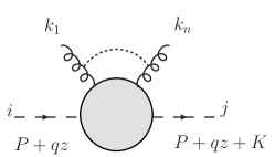
Figure 2: Two BCFW extended matter particles and many gluons

Our first aim is to examine the possible color-structures that can emerge in the amplitude shown in figure 2. We will perform our analysis for scalars first and then generalize it to include fermions.

Our treatment here is similar to [22]. To study the large $z$ behavior of the tree amplitudes in figure 2, we adopt the space-cone gauge of [34] that was used to analyze QCD amplitudes in [35]. This was called the q-lightcone gauge in [22]. We choose a gauge, so that the gauge field satisfies

$$q\cdot A(l)=0,\quad\text{for~{}}q\cdot l\neq 0.$$ (46)

If we also choose the gauge-boson propagator to satisfy $q_{\mu}\Pi^{\mu\nu}(l)=0$, for $q\cdot l\neq 0$ then, at large $z$, the tree-amplitude in Fig 2 is dominated by diagrams that have a small number of gluon-scalar vertices. This is because each scalar propagator comes with a factor of ${\rm O}\left({1\over z}\right)$, while factors of $z$ in the numerator can only come from interactions with a gluon line that carries the momentum $K$.

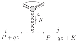
Figure 3: Dominant diagram at large z

Hence, in this gauge, the leading contribution to the tree amplitude in figure 2 is given by the diagram shown in Fig 3 This leads to a contribution

$$i\left[(2P+K+2qz)\cdot A^{a}(K)\right]T^{a}_{ji}.$$

In this and other diagrams below, the gluon lines that interact with the scalar could come from external gluons. Alternately, they could come from a gluon propagator that connects to the external gluons through the blobs shown in the diagrams. Since these details are not important for counting powers of $z$, we have parametrized the interactions of the scalars with the gluon lines through background vectors $A^{a}(l_{i})$ carrying momentum $l_{i}$ and the color index $a$.

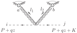
Figure 4: Contact interaction at ${\rm O}\left({z^{0}}\right)$

Proceeding to ${\rm O}\left({z^{0}}\right)$, we find that the contact interaction can also contribute. This leads to a contribution

$$i\left[A^{a}(l_{1})\cdot A^{b}(l_{2})\right]\{T^{a},T^{b}\}_{ji}.$$

In fact, by drawing a few more such diagrams one quickly finds a pattern emerging. Each diagram gives us a product of generators. Using the commutation relations of the algebra, we can express this product in terms of completely symmetrized products and the structure constants. We find that the leading contribution to the symmetrized product of $p$ generators comes with the power $z^{2-p}$. More precisely, an amplitude with $n$ gluons and two scalars — $s^{-}$ carrying color index $i$ and $s^{+}$ carrying color index $j$ — as shown in figure 2 is of the form

$${\mathcal{A}}(s^{-},s^{+},\ldots)=\sum_{p=1}^{n}{c_{a_{1}\ldots a_{p}}\over z^{p-2}}\left[T^{(a_{1}}\ldots T^{a_{p})}\right]_{ji}.$$ (47)

The $c$’s are rational functions of the external kinematic invariants, with the property that they do not diverge at large $z$, and are independent of the representation in which the scalars transform. Here, we provide a formal proof of this statement. The reader who prefers diagrams in q-lightcone gauge is referred to appendix B for further explicit calculations.

We will prove the statement (47) via induction. Note, that with one gluon the amplitude is of the form above. Now, assume that the form (47) is true for amplitudes with up to $n$ gluons. We will show that this implies that it is true for an amplitude with $n+1$ gluons.

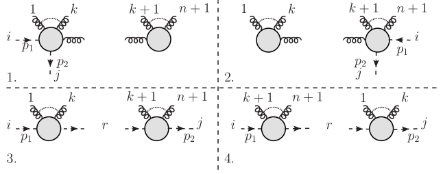
Figure 5: Four terms in the recursion relation

The amplitude with $n+1$ gluons can be calculated via BCFW recursion. Let us extend the 1^st and (n+1)^th gluon. So, we consider the BCFW extension $k_{1}\rightarrow k_{1}+tw,k_{n+1}\rightarrow k_{n+1}-tw$, as a function of the parameter $w$ (separate from $z$). We now find 4 types of terms. These are shown in figure 5 (where $p_{1}\equiv P+qz,p_{2}\equiv P+qz+K$).

• Terms where the last gluon is paired with $n-k$ other gluons. The intermediate particle is a gluon and the other gluons and both the scalars are paired with the first gluon.

• Terms where the first gluon is paired with $k-1$ other gluons. The intermediate particle is a gluon and the other gluons and both the scalars are paired with the last gluon.

• Terms where the $s^{-}$ is paired with the first gluon and $k-1$ other gluons and the intermediate cut particle is a scalar.

• Terms where the $s^{-}$ is paired with the last gluon and $n-k$ other gluons and the intermediate cut particle is a scalar.

The first two kinds of terms in the list above, clearly maintain the form 47. Consider the third term. If we club the first gluon with $k-1$ other gluons and $s^{-}$, we find a pole when $w$ takes the value $w_{0}=-{q\cdot(\sum_{i=1}^{k}k_{i})\over q\cdot t}+{\rm O}\left({1\over z}\right)$. So, the third term gives us a contribution to the amplitude of the form

$${1+{\rm O}\left({1\over z}\right)\over 2zq\cdot\sum_{i=1}^{k}k_{i}}\left[\sum_{p=1}^{k}{c^{1}_{a_{1}\ldots a_{p}}\over z^{p-2}}T^{(a_{1}}\ldots T^{a_{p})}_{ri}\sum_{m=1}^{n+1-k}{c^{2}_{a_{1}\ldots a_{m}}\over z^{m-2}}T^{(a_{1}}\ldots T^{a_{m})}_{jr}\right].$$ (48)

To the left, we have the propagator factor as in (8) and in the square bracket we have the product of the two amplitudes that, by hypothesis, have the form (47). Now, the $c$’s in the expression above are rational functions of the momentum associated with $s^{-}$ — $P+qz$ — and the spinors associated with the gluons. More precisely, the $c$’s can depend on dot products of $P+qz$ with the external polarization vectors and partial sums of the momenta that appear in the amplitude. Each of these terms is ${\rm O}\left({z}\right)$ and its dependence on $P$ is subleading. The only term we need to worry about is $(P+qz)\cdot(P+qz+K^{\prime})$ where $K^{\prime}=\sum_{i=1}^{k}k_{i}+tw_{0}$. However, we have

$$(P+qz)\cdot(P+qz+K^{\prime})=(P+qz)\cdot K^{\prime}=-{(K^{\prime})^{2}\over 2},$$ (49)

which is also independent of $P$ to leading order. In particular, this means that to leading order in $z$, the coefficients $c^{1},c^{2}$ are independent of $P$. This will be important for us below.

The fourth term involves a pole at $w_{1}=-{q\cdot(\sum_{i=1}^{k}k_{i})\over q\dot{t}}+{\rm O}\left({1\over z}\right)$. So $w_{1}-w_{0}={\rm O}\left({1\over z}\right)$. This amplitude now gives us a term of the form

$${-1+{\rm O}\left({1\over z}\right)\over 2zq\cdot\sum_{i=1}^{k}k_{i}}\left[\sum_{p=1}^{k}{c^{3}_{a_{1}\ldots a_{p}}\over z^{p-2}}T^{(a_{1}}\ldots T^{a_{p})}_{jr}\sum_{m=1}^{n+1-k}{c^{4}_{a_{1}\ldots a_{m}}\over z^{m-2}}T^{(a_{1}}\ldots T^{a_{m})}_{ri}\right].$$ (50)

However, the coefficients $c^{i}$ must satisfy

$$c^{1}-c^{3}={\rm O}\left({1\over z}\right)\quad c^{2}-c^{4}={\rm O}\left({1\over z}\right).$$ (51)

This is because they are both associated with the amplitude of a BCFW extended scalar shooting through a set of gluons. Up to terms of ${\rm O}\left({1\over z}\right)$, the gluons have the same momentum in two two cases since $w_{1}=w_{0}+{\rm O}\left({1\over z}\right)$. The subleading terms in the scalar momenta differ but as argued above, these only affect the ${\rm O}\left({1\over z}\right)$ terms in the $c$’s which are rational functions of the external scalar momenta.

This means that the amplitude with $n+1$ gluons is of the form,

$$\begin{split}&\sum_{p=1}^{k}\sum_{m=1}^{n-k+1}{1\over 2q\cdot\sum_{i=1}^{k}k_{i}}\left[{c^{1}_{a_{1}\ldots a_{p}}c^{2}_{a_{1}\ldots a_{m}}+{\rm O}\left({1\over z}\right)\over z^{p+m-3}}[T^{(a_{1}}\ldots T^{a_{m})},T^{(a_{1}}\ldots T^{a_{p})}]_{ji}\right]\\ &+{\rm O}\left({1\over z^{p+m-2}}\right)\{T^{(a_{1}}\ldots T^{a_{p})},T^{(a_{1}}\ldots T^{a_{m})}\}_{ji}.\end{split}$$ (52)

However, the commutator in (52) can be expressed in terms of a symmetrized product of at most $p+m-1$ generators. This proves our result.

We can prove a very similar result for fermions. The only subtlety here is that the fermionic amplitude is a rational function, not of the external fermionic momenta, but of the spinors that we associate to the two matter lines in figure 2. We are interested in the case where this amplitude comes from cutting a loop diagram. However, as we mentioned in footnote 2, in cutting a loop line we can choose to decompose the cut momenta $p$ into a convenient pair of spinors $p_{\alpha\dot{\alpha}}=\lambda_{\alpha}\bar{\lambda}_{\dot{\alpha}}$ provided that when we encounter $-p$ in another tree-amplitude associated with the cut, we maintain consistency with (15) by decomposing it as $-p=(-\lambda_{\alpha})\bar{\lambda}_{\dot{\alpha}}$.

We use this freedom to make the choice that we decompose the two large BCFW momenta in figure 2 as

$$\begin{split}(P+qz)_{\alpha\dot{\alpha}}&=(\lambda z+\lambda_{s}^{1})_{\alpha}(\bar{\lambda}+{\bar{\lambda}_{s}^{1}\over z})_{\dot{\alpha}}\\ -(P+qz+K)_{\alpha\dot{\alpha}}&=(-\lambda z-\lambda_{s}^{2})_{\alpha}(\bar{\lambda}+{\bar{\lambda}_{s}^{2}\over z})_{\dot{\alpha}}.\end{split}$$ (53)

Here, $\lambda_{s}^{i},\bar{\lambda}_{s}^{i}$ are some subleading terms that can depend on $z$ but must remain finite as $z\rightarrow\infty$. With the sign convention described above, this decomposition can be consistently imposed on all the tree-amplitudes that appear in the calculation of a bubble or a triangle coefficient.

Note that once we specify $\lambda_{s}^{1},\bar{\lambda}_{s}^{1}$ then $\lambda_{s}^{2}$ and $\bar{\lambda}_{s}^{2}$ are completely fixed by the external gluon momenta. By an extension of the argument given for scalars above, the dependence of $c$ on $\lambda_{s}^{1},\bar{\lambda}_{s}^{1}$ is subleading in $z$. With this observation, it is easy to repeat the proof above and show that subject to the decomposition (53), fermionic amplitudes also obey (47).

5.2 Contribution of Matter to Bubbles

We now have all the tools in hand to analyze the contribution of matter to individual bubble coefficients. We recall from section 4.2 that a bubble coefficient is calculated by making a cut and taking the product of the two tree-amplitudes,

$$C=\int d\Omega\oint_{z=\infty}{dz\over 2\pi iz}\sum{\mathcal{A}}^{\rm t}_{\rm left}(p_{1}+qz,-p_{2}-qz,\ldots){\mathcal{A}}^{\rm t}_{\rm right}(-p_{1}-qz,p_{2}+qz,\ldots).$$ (54)

Here $p_{1},p_{2}$ denote the two cut momenta and $q\cdot p_{1}=q\cdot p_{2}=0$. The sum is over the set of intermediate cut-particles (as, for example, in (43)) and the integral is over the phase-space associated with the cut.

From our analysis above, both ${\mathcal{A}}^{\rm t}_{\rm left}$ and ${\mathcal{A}}^{\rm t}_{\rm right}$ have the form of (47). Hence the contribution of scalars or fermions to the bubble coefficient is given by

$$\begin{split}C=(-1)^{F}\int d\Omega\oint_{z=\infty}{dz\over 2\pi iz}&\left[z^{2}c^{l}_{a_{1}}c^{r}_{a_{2}}{\rm Tr}(T^{a_{1}}T^{a_{2}})\right.\\ &+\left.\left(c^{l}_{a_{1}a_{2}}c^{r}_{a_{3}a_{4}}+c^{r}_{a_{1}a_{2}}c^{l}_{a_{3}a_{4}}\right){\rm Tr}(T^{(a_{1}}T^{a_{2})}T^{(a_{3}}T^{a_{4})})\right.\\ &+\left.\left(c^{l}_{a_{1}a_{2}a_{3}}c^{r}_{a_{4}}+c^{r}_{a_{1}a_{2}a_{3}}c^{r}_{a_{4}}\right){\rm Tr}(T^{(a_{1}}T^{a_{2}}T^{a_{3})}T^{a_{4}})\right],\end{split}$$ (55)

where $c^{l}$ and $c^{r}$ are associated with ${\mathcal{A}}^{\rm t}_{\rm left}$ and ${\mathcal{A}}^{\rm t}_{\rm right}$ respectively, in the expansion (47).

We can interchange the partially symmetrized traces in (55) for completely symmetrized traces at the cost of some structure constants. Hence, after doing the integral over $z$ and the phase space in (55), we find that the contribution of scalars/fermions in the representation $R_{s}/R_{f}$ can be written as

$$C_{s/f}=\sum_{n=2,4}\omega_{a_{1}\ldots a_{n}}{\rm Tr}_{R_{s}/R_{f}}(T^{(a_{1}}\ldots T^{a_{n})}),$$ (56)

where the $\omega$ are some coefficients that are independent of the representations $R_{s}/R_{f}$.

If we have a complex scalar running in the loop, (54) tells us that the loop receives a separate contribution from its complex conjugate. This contribution is the same, in every respect, except that we must modify the generators by $T^{a}\rightarrow-(T^{a})^{T}$. To keep this manifest at every step we will adopt the slightly unusual convention that whenever we write ${\rm Tr}_{R_{s}}$, we count a complex scalar and its conjugate as separate representations in $R_{s}$. This means, for example, that a scalar transforming in the fundamental representation of $SU(N)$ will be represented using $R_{s}={\bf N}+\overline{\bf N}$. This convention also allows us to treat complex and real (or pseudoreal) representations uniformly later. Moreover, it is immediately clear that the symmetrized product of three generators never appears in (56) above since $R_{s}$ must be self-conjugate. With chiral fermions, the odd symmetrized products do not vanish automatically. However, the symmetrized trace of three generators in $R_{f}$ must vanish for the theory to be anomaly free; so we have excluded this contribution from (56).

5.2.1 A small detour

This expression can be put in a slightly nicer form that reveals its dependence on various invariants of the algebra. We will take a small detour into group-theory to do this. So far our discussion has been valid for semi-simple groups. In this section, we focus on simple groups. Recall, that for any representation $R$,

$${\rm Tr}_{R}(T^{a}T^{b})=I_{2}(R)\kappa^{ab},$$ (57)

where $\kappa^{ab}$ is the Killing form. The coefficient $I_{2}(R)$ is called the (quadratic) Index and is commonly encountered in the calculation of the one-loop $\beta$ function. Similarly, for $SU(N)$ it is conventional to define

$${1\over 2}{\rm Tr}_{F}\left(T^{a}\{T^{b}T^{c}\}\right)\equiv d^{abc},$$ (58)

in the fundamental representation. Then, for any representation $R$

$${1\over 2}{\rm Tr}_{R}\left(T^{a}\{T^{b},T^{c}\}\right)=I_{3}(R)d^{abc}.$$ (59)

$I_{3}(R)$ — the third-order Index — is commonly called the anomaly.

In exactly the same way, for the fourth order trace we have [36]

$${\rm Tr}_{R}\left(T^{(a}T^{b}T^{c}T^{d)}\right)=I_{4}(R)d^{abcd}+I_{2,2}(R)\kappa^{(ab}\kappa^{cd)},$$ (60)

where $d^{abcd}$ are some suitably defined completely symmetric reference tensors. The coefficients $I_{4}(R)$ and $I_{2,2}(R)$ are called the fourth order Indices of the representation. We refer the reader to appendix A for further group theoretic details.

Substituting this expansion into (56), we find that we can write

$$C=I_{2}(R)\omega_{a_{1}a_{2}}\kappa^{a_{1}a_{2}}+I_{4}(R)\omega_{a_{1}a_{2}a_{3}a_{4}}d^{a_{1}a_{2}a_{3}a_{4}}+I_{2,2}(R)\omega_{a_{1}a_{2}a_{3}a_{4}}\kappa^{(a_{1}a_{2}}\kappa^{a_{3}a_{4})}.$$ (61)

In this equation all the dependence on the representation $R$ has been captured by the three indices $I_{2},I_{4},I_{2,2}$. Hence, the contribution of matter in a given representation to individual bubble coefficients can depend on up to the fourth order Indices of the representation!

This is related to the result that matter in a representation $R$ contributes to the one-loop $\beta$ function through the second order Index. The only ultra-violet divergent diagrams in (32) are the bubbles. However, any one-loop amplitude receives contributions from several distinct bubble coefficients. Each bubble coefficient corresponds to a partition of the external momenta as in (38). With $q_{\alpha_{2}}$ defined in (39) for a given partition indexed by $\alpha_{2}$, the ultra-violet divergent piece of a one-loop amplitude is

$${\mathcal{A}}^{1l}_{UV}=\sum{C_{\alpha_{2}}\over 32\pi^{2}}\ln{\Lambda^{2}\over q_{\alpha_{2}}^{2}}.$$ (62)

While each $C_{\alpha_{2}}$ is individually important for the one-loop amplitude, the total UV-divergence depends only on the sum $\sum_{\alpha_{2}}C_{\alpha_{2}}$. In fact this sum must be proportional to the tree amplitude for scattering of the external gluons [5].

Hence, while individual bubble coefficients depend on the higher order Indices and are not necessarily proportional to the tree-amplitude the sum of all bubble coefficients is proportional to the product of the tree amplitude and the second order Index! In fact, the extra UV divergences that appear in individual bubble coefficients are a bit like the ‘spurious poles’ [17] that appear in tree amplitudes; they cancel when we add all contributing terms. We verify this in section 7 but it would be nice to have a direct proof of this fact.

What about scalars in the adjoint representation? Is it true that, at least, for this kind of matter the bubble coefficient is proportional to the tree-amplitude? From our analysis in this subsection, we cannot answer this question. However, our explicit calculations in section 7.2 will show us that, even with adjoint matter, the contribution of matter to a bubble coefficient is not proportional to the tree-amplitude. Miraculously, when we add up all bubble coefficients, the ultra-violet divergent term at one-loop is proportional to the tree-amplitude!

5.3 Contribution of Matter to Triangles

Now, we consider the contribution of matter to triangles. Recall, from section 4.1 that the triangle coefficient is calculated by making a 3-cut and calculating the product of three tree-amplitudes

$$B=\sum_{\pm}\oint_{z=\infty}{dz\over 4\pi\sqrt{r^{2}-z^{2}}}A^{\rm t}(p_{1}^{\pm}(z),-p_{2}^{\pm}(z),\ldots)A^{\rm t}(-p_{1}^{\pm}(z),p_{3}^{\pm}(z),\ldots)A^{\rm t}(p_{2}^{\pm}(z),-p_{3}^{\pm}(z),\ldots).$$ (63)

Here, as described in more detail in section 4.1, $p_{i}^{\pm}(z)$ are null-vectors and for large $z$, $p_{i}^{\pm}(z)\rightarrow q^{\pm}z$ where $q^{\pm}$ are also null.

We can see from a simple extension of the analysis that we performed above that for the contributions of scalars in a representation $R_{s}$, or of fermions in a representation $R_{f}$, to a triangle coefficient we can write

$$B_{s/f}=\sum_{n=2,4,5,6}\omega_{a_{1}\ldots a_{n}}{\rm Tr}_{R_{s}/R_{f}}(T^{(a_{1}}\ldots T^{a_{n})}).$$ (64)

Hence, the contribution to matter to triangles can involve up to the sixth order Indices of the matter representation.

5.4 Simplifications in Supersymmetric Theories

We now describe a remarkable simplification that occurs in supersymmetric theories. In theories, with at least ${\mathcal{N}}=1$ supersymmetry, in each individual bubble coefficient, the contribution of fermions to the fourth order Indices exactly cancels the contribution of scalars. Similarly, in each individual triangle coefficient, the contribution of fermions to the sixth order Indices exactly cancels the contribution of scalars.

This means that for supersymmetric theories, each individual bubble and triangle coefficient can be written as

$$C=\omega^{C}_{a_{1}a_{2}}I_{2}(R)\kappa^{a_{1}a_{2}},\quad B=\sum_{n=2,4,5}\omega^{B}_{a_{1}\ldots a_{n}}{\rm Tr}_{R}(T^{(a_{1}}\ldots T^{a_{n})}).$$ (65)

If the chiral multiplets are in self-conjugate representations (this is automatic if they are part of ${{\mathcal{N}}=2}$ hypermultiplets), then the term with $n=5$ is also absent in (65).

This happens because, subject to the scaling choice (53), the coefficients for fermions and scalars in the expansion (47) satisfy

$$c^{s}-c^{f}={\rm O}\left({1\over z}\right).$$ (66)

We sketch a proof of this using supersymmetry. This proof is completed in appendix B which also contains some explicit calculations that verify (66) for the coefficients of symmetrized products involving up to 3 generators.

First, notice that we can embed the amplitude of figure 2 in a supersymmetric theory. Since all our external particles are gluons, the gauginos are just spectators. With the supersymmetric version of the chiral multiplet introduced in section 3.4, we can write this amplitude as

$${\mathcal{A}}^{\rm t}(\{0^{-},\eta_{1},\lambda_{1}(z),\bar{\lambda}_{1}(z)\},\{0^{+},\eta_{2},\lambda_{2}(z),\bar{\lambda}_{2}(z)\}\ldots\{b_{i},0,\lambda_{i},\bar{\lambda}_{i}\},\ldots),$$ (67)

where the $b_{i}=\pm 1$ represent gluons with either negative or positive helicity. The spinors $\lambda_{1},\bar{\lambda}_{1}$ and $\lambda_{2},\bar{\lambda}_{2}$ are chosen according to (53).

Now, consider a supersymmetry transformation $e^{\left\langle Q,\chi\right\rangle}$, with

$$\chi={\eta_{2}w\over z},\quad\langle w,{\lambda_{2}\over z}\rangle=1.$$ (68)

$w$ is not uniquely defined above since we can add any multiple of $\lambda_{2}$ to $w$ but this ambiguity will not affect us below provided we ensure that for large $z$, $w\rightarrow{\rm O}\left({1}\right)$. This implies $\chi\rightarrow{\rm O}\left({1\over z}\right).$

Demanding that the amplitude in (67) be invariant under this supersymmetry transformation leads to

$$\begin{split}&{\mathcal{A}}^{\rm t}(\{0^{-},\eta_{1},\lambda_{1}(z),\bar{\lambda}_{1}(z)\},\{0^{+},\eta_{2},\lambda_{2}(z),\bar{\lambda}_{2}(z)\}\ldots\{b_{i},0,\lambda_{i},\bar{\lambda}_{i}\},\ldots)\\ &=e^{\left\langle Q,\chi\right\rangle}{\mathcal{A}}^{\rm t}(\{0^{-},\eta_{1},\lambda_{1}(z),\bar{\lambda}_{1}(z)\},\{0^{+},\eta_{2},\lambda_{2}(z),\bar{\lambda}_{2}(z)\}\ldots\{b_{i},0,\lambda_{i},\bar{\lambda}_{i}\},\ldots)\\ &=e^{\phi}{\mathcal{A}}^{\rm t}(\{0^{-},\eta_{1},\lambda_{1}(z),\bar{\lambda}_{1}(z)\},\{0^{+},0,\lambda_{2}(z),\bar{\lambda}_{2}(z)\}\ldots\{b_{i},\eta_{i}^{\prime},\lambda_{i},\bar{\lambda}_{i}\},\ldots),\end{split}$$ (69)

where

$$\phi={\left\langle\lambda_{1},w\right\rangle\over z}\eta_{2}\eta_{1}=\eta_{2}\eta_{1}\left(1+{\rm O}\left({1\over z}\right)\right),\quad\eta_{i}^{\prime}=-\eta_{2}{\left\langle w,\lambda_{i}\right\rangle\over z},~{}{\rm if}~{}b_{i}=-1.$$ (70)

We can now series expand the last line of (69) in the $\eta_{i}^{\prime}$. The leading term in this expansion has only gluons and no gauginos. Since, particle $2$ is now a scalar and since there are no external gauginos, particle $1$ must also be a scalar. The term proportional to $\eta_{i}^{\prime}$ involves a gaugino in position $i$ and leads to an amplitude involving a chiral multiplet scalar, a negative helicity chiral multiplet fermion and a negative helicity vector multiplet gaugino. However, this amplitude is suppressed by ${1\over z}$!

$$\begin{split}&{\mathcal{A}}^{\rm t}(\{0^{-},\eta_{1},\lambda_{1}(z),\bar{\lambda}_{1}(z)\},\{0^{+},\eta_{2},\lambda_{2}(z),\bar{\lambda}_{2}(z)\}\ldots\{b_{i},0,\lambda_{i},\bar{\lambda}_{i}\},\ldots)\\ &=\left[1+\eta_{2}\eta_{1}\left(1+{\rm O}\left({1\over z}\right)\right)\right]{\mathcal{A}}^{\rm t}(\{0^{-},0,\lambda_{1}(z),\bar{\lambda}_{1}(z)\},\{0^{+},\eta_{2},\lambda_{2}(z),\bar{\lambda}_{2}(z)\}\ldots\{b_{i},\eta_{i}^{\prime},\lambda_{i},\bar{\lambda}_{i}\},\ldots)\\ &=\left[1+\eta_{2}\eta_{1}\left(1+{\rm O}\left({1\over z}\right)\right)\right]{\mathcal{A}}^{\rm t}(\{0^{-},0,\lambda_{1}(z),\bar{\lambda}_{1}(z)\},\{0^{+},0,\lambda_{2}(z),\bar{\lambda}_{2}(z)\}\ldots\{b_{i},0,\lambda_{i},\bar{\lambda}_{i}\},\ldots)\\ &+{R\over z}.\end{split}$$ (71)

If $b_{3}=-1$, then $R$ includes a term

$${\eta_{2}\eta_{1}\over z}{\mathcal{A}}^{\rm t}(\{f^{-},\lambda_{1}(z),\bar{\lambda}_{1}(z)\},\{s^{+},\lambda_{2}(z),\bar{\lambda}_{2}(z)\},\{\psi^{-},\lambda_{3},\bar{\lambda}_{3}\},\{g^{\pm},\lambda_{4},\bar{\lambda}_{4}\}\ldots),$$

and similar terms for each negative $b_{i}$. To complete the proof, we need to show that $R$ does not contain a contribution to the $k^{\rm th}$ symmetrized product that scales faster than ${1\over z^{k-2}}$. We show this in appendix B.

The argument above proves our result, since the coefficient of $\eta_{2}\eta_{1}$ in (67) gives us the amplitude with fermions while the coefficient of $1$ gives us the amplitude with scalars.

We should emphasize here that it is not the case that the scalar and fermion amplitudes are equal. In fact, the ${\rm O}\left({1\over z}\right)$ terms in (66) can and do contribute to both bubble and triangle coefficients. However, in the consideration of the fourth order Indices for bubbles, as (55) tells us, it is only the leading terms in $c$ that are important. Similarly, while calculating the contribution to the sixth order Indices in a triangle coefficient it is only the leading terms in $c$ that can contribute. Since, the fermion loop comes with a negative sign, this implies that the matter contribution of a chiral multiplet to bubble coefficients does not depend on the fourth-order Indices. Similarly, the matter contribution of a chiral multiplet to triangle coefficients does not depend on the sixth order Indices.

6 The Next to Simplest Quantum Field Theories

In the previous section we argued that the contribution of matter in a given representation to individual bubble and triangle coefficients is dependent on a small set of group-theoretic invariants. Now, we also know that there are no triangles or bubbles in the ${\mathcal{N}}=4$ theory. However, we can think of the ${\mathcal{N}}=4$ theory itself as a gauge theory with matter in the adjoint representation. The contribution of matter is such that it exactly cancels out the contribution of the gauge bosons to bubbles and triangles. This leads to an interesting possibility: what if we find a representation that mimics the higher order Indices of the adjoint representation? We could then replace the adjoint fields of the ${{\mathcal{N}}=4}$ theory with fields in this representation and still get a simple S-matrix!

Let us state this a little more explicitly. Let us call the contribution of scalars in a representation ${\rm R}_{s}$ to the bubble coefficient $C^{s}({\rm R}_{s},k_{1},\ldots k_{n},r_{1},\ldots r_{n})$ and the contribution to the triangle coefficient $B^{s}({\rm R}_{s},k_{1},\ldots k_{n},r_{1},\ldots r_{n})$ The notation emphasizes that this coefficient depends on the external momenta $k_{i}$ (we have suppressed the helicity dependence), the colors of the external gluons $r_{i}$ and the representation ${\rm R}_{s}$. We denote the contributions of gluons and fermions by $C^{g},B^{g}$, $C^{f}$ and $B^{f}$.

We know from the previous section that

$$\begin{split}C_{s/f}(R_{s/f},k_{i},r_{i})&=\sum_{n=2,4}\omega^{C}_{a_{1}\ldots a_{n}}\left(k_{i},r_{i}\right){\rm Tr}_{R_{s}/R_{f}}(T^{(a_{1}}\ldots T^{a_{n})}),\\ B_{s/f}(R_{s/f},k_{i},r_{i})&=\sum_{n=2,4,5,6}\omega^{B}_{a_{1}\ldots a_{n}}\left(k_{i},r_{i}\right){\rm Tr}_{R_{s}/R_{f}}(T^{(a_{1}}\ldots T^{a_{n})}),\end{split}$$ (72)

where $\omega^{B}$ and $\omega^{C}$ are independent of $R_{s}$ and $R_{f}$ but depend on $k_{i},r_{i}$. However we also know, from the fact that there are no bubbles or triangles in the ${\mathcal{N}}=4$ theory that

$$\begin{split}&C^{g}(k_{i},r_{i})+4C^{f}({\rm A},k_{i},r_{i})+6C^{s}({\rm A},k_{i},r_{i})=0,\\ &B^{g}(k_{i},r_{i})+4B^{f}({\rm A},k_{i},r_{i})+6B^{s}({\rm A},k_{i},r_{i})=0,\end{split}$$ (73)

where we have denoted the adjoint representation by ${\rm A}$. So, we wish to find representations $R_{s},R_{f}$ with the property

$$\begin{split}{\rm Tr}_{R_{s}}\left(\Pi_{i=1}^{n}T^{a_{i}}\right)&=6{\rm Tr}_{A}\left(\Pi_{i=1}^{n}T^{a_{i}}\right),\forall n\leq p\\ {\rm Tr}_{R_{f}}\left(\Pi_{i=1}^{n}T^{a_{i}}\right)&=4{\rm Tr}_{A}\left(\Pi_{i=1}^{n}T^{a_{i}}\right),\forall n\leq p.\end{split}$$ (74)

If we can find solutions for $p=6$ that would give us a theory that is free of triangles and bubbles. If we can find a solution for $p=4$ that would still be sufficient to give us a theory without bubbles.

These conditions simplify for supersymmetric theories. For a chiral multiplet $\chi$ in a representation $R_{\chi}$ we know that

$$\begin{split}C_{\chi}(R_{\chi},k_{i},r_{i})&=\omega^{C}_{a_{1}a_{2}}\left(k_{i},r_{i}\right){\rm Tr}_{R_{\chi}}(T^{a_{1}}T^{a_{2}}),\\ B_{\chi}(R_{\chi},k_{i},r_{i})&=\sum_{n=2,4,5}\omega^{B}_{a_{1}\ldots a_{n}}\left(k_{i},r_{i}\right){\rm Tr}_{R_{\chi}}(T^{(a_{1}}\ldots T^{a_{n})}),\end{split}$$ (75)

Furthermore, thinking of the ${\mathcal{N}}=4$ theory as a ${\mathcal{N}}=1$ theory with 3 chiral multiplets and denoting the vector multiplet by $V$, we know that

$$\begin{split}&C^{V}(k_{i},r_{i})+3C^{\chi}({\rm A},k_{i},r_{i})=0,\\ &B^{V}(k_{i},r_{i})+3B^{\chi}({\rm A},k_{i},r_{i})=0.\end{split}$$ (76)

So, in supersymmetric theories we need to put the chiral multiplet in a representation $R_{\chi}$ that satisfies

$${\rm Tr}_{R_{\chi}}\left(\Pi_{i=1}^{n}T^{a_{i}}\right)=3{\rm Tr}_{A}\left(\Pi_{i=1}^{n}T^{a_{i}}\right),\forall n\leq p.$$ (77)

Now a solution for $p=2$ is enough to give us a theory without bubbles while a solution for $p=5$ is enough to give us a theory with neither bubbles nor triangles. For the convenience of the reader we have summarized all the different conditions above in Table 1.

Condition (C): ${\rm Tr}_{\rm R}(\Pi_{i=1}^{n}T^{a_{i}})=m\,{\rm Tr}_{\rm adj}(\Pi_{i=1}^{n}T^{a_{i}}),~{}n\leq p$
Non-susy theories have	only boxes	no bubbles
if $R_{f}$ satisfies C with	p=6, m=4	p=4,m=4
and $R_{s}$ satisfies C with	p=6, m=6	p=4,m=6.
Susy theories have	only boxes	no bubbles
if $R_{\chi}$ satisfies C with	p=5, m=3	p=2,m=3.

Table 1: Conditions for the S-matrix to simplify

These equations for the absence of bubbles and triangles have a nice interpretation in terms of the Indices that we discussed earlier. The representations $R_{s},R_{f}$ and $R_{\chi}$ that we have been talking about above can be decomposed into irreducible representations

$$R=\bigoplus n_{i}^{s}R_{i}.$$ (78)

Since Indices are additive (this is just because ${\rm Tr}_{R_{1}\oplus R_{2}}={\rm Tr}_{R_{1}}+{\rm Tr}_{R_{2}}$), (74) or (77) are equivalent to a set of linear Diophantine equations in the variables $n_{i}$ that involve the higher-order Indices of the irreducible representations $R_{i}$!

We now present some solutions to these equations. Some further group-theoretic details are provided in appendix A.

6.1 Theories with only Boxes

We have been able to find solutions to (77) for $p\leq 5$.

Consider the ${\mathcal{N}}=2$, $SU(N)$ (for $N\geq 3$) theory with a hypermultiplet that transforms in the symmetric tensor representation of $SU(N)$ and another hypermultiplet that transforms as the anti-symmetric tensor. In ${{\mathcal{N}}=1}$ language, this leads to

$$\begin{split}{\rm R}_{\chi}&=\cdot{\bf adj}\oplus\cdot{\bf sym}\oplus{\bf asym}\oplus{\rm{\overline{\bf sym}}}\oplus{\rm\overline{\bf asym}}.\end{split}$$ (79)

We provide more details in appendix A but the reader can verify that, with this choice of representations, (77) is satisfied. So, this theory has neither bubbles nor triangles in its one-loop gluon S-matrix!

Note that gluon amplitudes, at one-loop, are not sensitive to the superpotential. As far as such amplitudes are concerned, a ${{\mathcal{N}}=1}$ theory with the same spectrum as the theory above will also be free of triangles and bubbles.

To take a more exotic example, consider a gauge theory based on the gauge-group $G_{2}$. The adjoint of $G_{2}$ is the $[{\bf 14}]$. If we consider the ${{\mathcal{N}}=1}$ theory, with a chiral multiplet in the representation

$$R_{\chi}=3\cdot[{\bf 7}]\oplus[{\bf 27}],$$ (80)

then also (77) is satisfied! So this gauge theory also has only boxes in its one-loop S-matrix!

Finally, we should mention that commonly studied superconformal theories like the ${\mathcal{N}}=2$, $SU(N)$ theory with $2N$ hypermultiplets or superconformal quiver gauge theories that are dual to orbifolds of $AdS_{5}\times S^{5}$ [37] generically contain fundamental (or bi-fundamental) matter in $SU(N)$. Individual triangle coefficients in such theories do not vanish since with scalars and fermions in a combination of just the fundamental and anti-fundamental representations of $SU(N)$, (77) cannot be satisfied for $p\geq 2$. However, at large $N$, these theories do provide approximate solutions to (77) as discussed in 6.3.

6.2 Theories without Bubbles

It is much easier to find theories without bubbles. First, note that the condition for supersymmetric theories to be free of bubbles, which is (77) with $p=2$, is just the condition for the one-loop $\beta$ function to vanish. So, any supersymmetric theory with vanishing one-loop $\beta$ function is free of bubbles at one-loop. This includes, of course, the ${\mathcal{N}}=2$, $SU(N)$ theory with $2N$ hypermultiplets.

More interestingly, we can also find non-supersymmetric examples of theories that do not have bubbles. For non-supersymmetric theories the condition that individual bubble coefficients vanish is considerably stronger than the condition for the one-loop $\beta$ function to vanish.

For example, consider the $SU(2)$ theory with the following content

$$R_{s}=14\cdot[{\bf 2}]+[{\bf 4}],\quad R_{f}=4\cdot[{\bf 3}].$$ (81)

This is a $SU(2)$ gauge theory with 7 complex scalar doublets and one scalar in the ${3\over 2}$ representation. We impose a reality condition on this last field. More explicitly, if we write this field as a symmetric 3-index tensor $\phi^{i_{1}j_{1}k_{1}}$ in a 2 dimensional space, then the reality condition is $\phi^{*}_{i_{2}j_{2}k_{2}}=\epsilon_{i_{1}i_{2}}\epsilon_{j_{1}j_{2}}\epsilon_{k_{1}k_{2}}\phi^{i_{1}j_{1}k_{2}}$. In addition, this theory has 4 adjoint Weyl fermions. Since (74) is met for $p\leq 4$, this theory does not have bubbles at one-loop!

Then we can derive other examples from the two supersymmetric theories that are free of both triangles and bubbles. For example, we could replace all the fermions in (79) with adjoint fermions. After including the adjoint fermions from the vector multiplet, this would lead to a theory with

$$\begin{split}{\rm R}_{s}&=2\cdot{\bf adj}\oplus 2\cdot{\bf sym}\oplus 2\cdot{\bf asym}\oplus 2\cdot{\rm{\overline{\bf sym}}}\oplus 2\cdot{\rm\overline{\bf asym}}.\\ {\rm R}_{f}&=4\cdot{\bf adj}\end{split}$$ (82)

Proceeding this way we can derive many other examples of non-supersymmetric theories without bubbles from the two theories of section 6.1.

We have not yet found representations ${\rm R}_{s}$ and ${\rm R}_{f}$ that would make triangles vanish for non-supersymmetric theories. However, it is possible to systematically search for such solutions and we provide a method to do so in appendix A.

6.3 Large N

The results about 1-loop gluon amplitudes that we have presented above hold exactly, without any need to take the planar limit. However, when the gauge group becomes large, it is possible to find new approximate solutions to (77).

For example, for $SU(N)$, at large N, the generators of the adjoint can be written as

$$T_{\rm adj}^{a}=T_{\rm f}^{a}\otimes 1+1\otimes(T_{\rm af}^{a}),\quad T_{\rm af}^{a}=-(T_{\rm f}^{a})^{T},$$ (83)

and so,

$${\rm Tr}\left(T_{\rm adj}^{(a_{1}}\ldots T_{\rm adj}^{a_{2n})}\right)=2N{\rm Tr}\left(T_{\rm f}^{(a_{1}}\ldots T_{\rm f}^{a_{2n})}\right)+\ldots,$$ (84)

where the $\ldots$ indicate terms that are subleading in $N$.

In particular, this tells us that the superconformal quiver gauge theories that are dual to orbifolds of AdS${}_{5}\times S^{5}$ are free of triangles and bubbles in the planar limit. This had to be, since these theories are daughters of the ${{\mathcal{N}}=4}$ theory and their planar correlation functions can be obtained from the ${{\mathcal{N}}=4}$ theory [16, 38, 39]. Note that (84) also implies that, at large $N$, gluon amplitudes in the ${{\mathcal{N}}=2}$, $SU(N)$ theory with $2N$ hypermultiplets are also free of triangles or bubbles.

7 Examples

We now provide several examples of concrete amplitudes. This somewhat lengthy list performs two roles. It helps to check the claims that we have made but also serves to elucidate the beautiful structure described above.

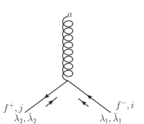
Figure 6: Fermion-gluon interaction

This section is divided in three parts. In subsection 7.1, we provide explicit calculations of tree amplitudes with 2 matter particles (scalars or fermions) and gluons. In subsection 7.2, we use these tree amplitudes to calculate the triangle and bubble coefficients that appear in $2\rightarrow 2$ gluon scattering. In subsection 7.3, we summarize the results of these calculations. The reader can skip directly to 7.3 and then turn back to 7.1 and 7.2 for details.

7.1 Tree Amplitudes with 2 matter particles

Here, we list the formulas for amplitudes involving two scalars or two fermions and up to 3 external gluons. We have stripped off a factor of $-i\left(-g_{YM}\right)^{n-2}$ from the $n$ point amplitude below.

7.1.1 3-pt Amplitudes

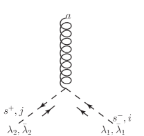
Figure 7: Scalar-gluon interaction

We use the following 3-pt amplitudes. For fermions, figure 6 evaluates to

$$\begin{split}{\mathcal{A}}^{\rm t}(f^{-},f^{+},g^{-})&=\sqrt{2}{\left\langle\lambda_{3},\lambda_{1}\right\rangle^{2}\over\left\langle\lambda_{1},\lambda_{2}\right\rangle}T^{a}_{ji},\\ {\mathcal{A}}^{\rm t}(f^{-},f^{+},g^{+})&=\sqrt{2}{[\bar{\lambda}_{3},\bar{\lambda}_{2}]^{2}\over[\bar{\lambda}_{2},\bar{\lambda}_{1}]}T^{a}_{ji}.\end{split}$$ (85)

For scalars, we have the figure 7

$$\begin{split}{\mathcal{A}}^{\rm t}(s^{-},s^{+},g^{-})&=\sqrt{2}{\left\langle\lambda_{2},\lambda_{3}\right\rangle\left\langle\lambda_{3},\lambda_{1}\right\rangle\over\left\langle\lambda_{1},\lambda_{2}\right\rangle}T^{a}_{ji},\\ {\mathcal{A}}^{\rm t}(s^{-},s^{+},g^{+})&=\sqrt{2}{[\bar{\lambda}_{2},\bar{\lambda}_{3}][\bar{\lambda}_{3},\bar{\lambda}_{1}]\over[\bar{\lambda}_{1},\bar{\lambda}_{2}]}T^{a}_{ji}.\end{split}$$ (86)

For completeness, we list the gluon 3-pt amplitudes

$$\begin{split}{\mathcal{A}}^{\rm t}(g^{-},g^{-},g^{+})&=\sqrt{2}{\left\langle\lambda_{1},\lambda_{2}\right\rangle^{3}\over\left\langle\lambda_{2},\lambda_{3}\right\rangle\left\langle\lambda_{3},\lambda_{1}\right\rangle}f^{123},\\ {\mathcal{A}}^{\rm t}(g^{-},g^{-},g^{+})&=\sqrt{2}{[\bar{\lambda}_{1},\bar{\lambda}_{2}]^{3}\over[\bar{\lambda}_{2},\bar{\lambda}_{3}][\bar{\lambda}_{3},\bar{\lambda}_{1}]}f^{123},\end{split}$$ (87)

in conventions where the structure constants are defined by

$$\left[T^{a},T^{b}\right]=f^{abc}\,T^{c}.$$ (88)

7.1.2 4-pt Amplitudes

The four point amplitudes for 2 fermions and gluons of the same helicity vanishes; the amplitude with gluons of opposite helicity is

$$\begin{split}{\mathcal{A}}^{\rm t}(f^{-},f^{+},g^{+},g^{-})={2{\left\langle\lambda_{1},\lambda_{4}\right\rangle}^{2}\over\left\langle\lambda_{3},\lambda_{4}\right\rangle\left\langle\lambda_{1},\lambda_{2}\right\rangle}\left({\left\langle\lambda_{2},\lambda_{4}\right\rangle\over\left\langle\lambda_{2},\lambda_{3}\right\rangle}\left(T^{a}T^{b}\right)_{ji}-{\left\langle\lambda_{1},\lambda_{4}\right\rangle\over\left\langle\lambda_{1},\lambda_{3}\right\rangle}\left(T^{b}T^{a}\right)_{ji}\right),\end{split}$$ (89)

where $g^{+}$ carries color $a$ and $g^{-}$ carries color $b$. The four point amplitude with 2 scalars and gluons of opposite helicities is

$$\begin{split}{\mathcal{A}}^{\rm t}(s^{-},s^{+},g^{+},g^{-})={2\left\langle\lambda_{4},\lambda_{1}\right\rangle\left\langle\lambda_{2},\lambda_{4}\right\rangle\over\left\langle\lambda_{3},\lambda_{4}\right\rangle\left\langle\lambda_{1},\lambda_{2}\right\rangle}\left({\left\langle\lambda_{2},\lambda_{4}\right\rangle\over\left\langle\lambda_{2},\lambda_{3}\right\rangle}\left(T^{a}T^{b}\right)_{ji}-{\left\langle\lambda_{1},\lambda_{4}\right\rangle\over\left\langle\lambda_{1},\lambda_{3}\right\rangle}\left(T^{b}T^{a}\right)_{ji}\right).\end{split}$$ (90)

7.1.3 5-pt Amplitudes

Finally, we turn to the 5-pt amplitude. With two gluons of positive helicity and one of negative helicity, this is

$$\begin{split}&{\mathcal{A}}^{\rm t}(f^{-},f^{+},g^{+},g^{+},g^{-})\\ &=\frac{-2\sqrt{2}\left\langle\lambda_{1},\lambda_{5}\right\rangle{}^{3}}{\left\langle\lambda_{1},\lambda_{2}\right\rangle\left\langle\lambda_{3},\lambda_{5}\right\rangle\left\langle\lambda_{4},\lambda_{5}\right\rangle\left\langle\lambda_{1},\lambda_{3}\right\rangle}\left(\frac{\left\langle\lambda_{2},\lambda_{5}\right\rangle(T^{b}T^{c}T^{a})_{ji}}{\left\langle\lambda_{2},\lambda_{4}\right\rangle}-\frac{\left\langle\lambda_{1},\lambda_{5}\right\rangle(T^{c}T^{b}T^{a})_{ji}}{\left\langle\lambda_{1},\lambda_{4}\right\rangle}\right)\\ &+\frac{2\sqrt{2}\left\langle\lambda_{2},\lambda_{5}\right\rangle\left\langle\lambda_{1},\lambda_{5}\right\rangle{}^{2}}{\left\langle\lambda_{1},\lambda_{2}\right\rangle\left\langle\lambda_{4},\lambda_{5}\right\rangle\left\langle\lambda_{3},\lambda_{5}\right\rangle\left\langle\lambda_{2},\lambda_{3}\right\rangle}\left(\frac{\left\langle\lambda_{2},\lambda_{5}\right\rangle(T^{a}T^{b}T^{c})_{ji}}{\left\langle\lambda_{2},\lambda_{4}\right\rangle}-\frac{\left\langle\lambda_{1},\lambda_{5}\right\rangle(T^{a}T^{c}T^{b})_{ji}}{\left\langle\lambda_{1},\lambda_{4}\right\rangle}\right)\\ &+\frac{2\sqrt{2}f^{abd}\left\langle\lambda_{1},\lambda_{5}\right\rangle{}^{2}}{\left\langle\lambda_{1},\lambda_{2}\right\rangle\left\langle\lambda_{3},\lambda_{4}\right\rangle\left\langle\lambda_{3},\lambda_{5}\right\rangle}\left(\frac{\left\langle\lambda_{2},\lambda_{5}\right\rangle(T^{d}T^{c})_{ji}}{\left\langle\lambda_{2},\lambda_{4}\right\rangle}-\frac{\left\langle\lambda_{1},\lambda_{5}\right\rangle(T^{c}T^{d})_{ji}}{\left\langle\lambda_{1},\lambda_{4}\right\rangle}\right),\end{split}$$ (91)

where the gluons carry colors $a,b,c$ respectively. The scalar amplitude, with the same choice of gluon helicities, is,

$$\begin{split}&{\mathcal{A}}^{\rm t}(s^{-},s^{+},g^{+},g^{+},g^{-})\\ &\frac{-2\sqrt{2}\left\langle\lambda_{2},\lambda_{5}\right\rangle\left\langle\lambda_{1},\lambda_{5}\right\rangle{}^{2}}{\left\langle\lambda_{1},\lambda_{2}\right\rangle\left\langle\lambda_{1},\lambda_{3}\right\rangle\left\langle\lambda_{3},\lambda_{4}\right\rangle\left\langle\lambda_{4},\lambda_{5}\right\rangle}\left(\frac{\left\langle\lambda_{1},\lambda_{5}\right\rangle(T^{c}T^{b}T^{a})_{ji}}{\left\langle\lambda_{1},\lambda_{4}\right\rangle}-\frac{\left\langle\lambda_{2},\lambda_{5}\right\rangle(T^{b}T^{c}T^{a})_{ji}}{\left\langle\lambda_{2},\lambda_{4}\right\rangle}\right)\\ &+\frac{2\sqrt{2}\left\langle\lambda_{2},\lambda_{5}\right\rangle{}^{2}\left\langle\lambda_{1},\lambda_{5}\right\rangle}{\left\langle\lambda_{1},\lambda_{2}\right\rangle\left\langle\lambda_{2},\lambda_{3}\right\rangle\left\langle\lambda_{3},\lambda_{5}\right\rangle\left\langle\lambda_{4},\lambda_{5}\right\rangle}\left(\frac{\left\langle\lambda_{1},\lambda_{5}\right\rangle(T^{a}T^{c}T^{b})_{ji}}{\left\langle\lambda_{1},\lambda_{4}\right\rangle}-\frac{\left\langle\lambda_{2},\lambda_{5}\right\rangle(T^{a}T^{b}T^{c})_{ji}}{\left\langle\lambda_{2},\lambda_{4}\right\rangle}\right)\\ &-\frac{2\sqrt{2}f^{abd}\left\langle\lambda_{1},\lambda_{5}\right\rangle\left\langle\lambda_{2},\lambda_{5}\right\rangle}{\left\langle\lambda_{1},\lambda_{2}\right\rangle\left\langle\lambda_{3},\lambda_{4}\right\rangle\left\langle\lambda_{3},\lambda_{5}\right\rangle}\left(\frac{\left\langle\lambda_{2},\lambda_{5}\right\rangle(T^{d}T^{c})_{ji}}{\left\langle\lambda_{2},\lambda_{4}\right\rangle}-\frac{\left\langle\lambda_{1},\lambda_{5}\right\rangle(T^{c}T^{d})_{ji}}{\left\langle\lambda_{1},\lambda_{4}\right\rangle}\right).\end{split}$$ (92)

Note, that we have

$${\mathcal{A}}^{\rm t}(f^{-},f^{+},g^{+},g^{+},g^{-})=-{\left\langle\lambda_{1},\lambda_{5}\right\rangle\over\left\langle\lambda_{2},\lambda_{5}\right\rangle}{\mathcal{A}}^{\rm t}(s^{-},s^{+},g^{+},g^{+},g^{-}).$$ (93)

The amplitudes with the other choice of helicities for the gluons may be obtained from the expressions given above by parity and charge conjugation.

For example, the scalar amplitude with the opposite helicities for gluons can be obtained by turning all the $\lambda$’s above into $\bar{\lambda}$’s.

$$\begin{split}&{\mathcal{A}}^{\rm t}(s^{-},s^{+},g^{-},g^{-},g^{+})\\ &=\frac{-2\sqrt{2}[\bar{\lambda}_{2},\bar{\lambda}_{5}][\bar{\lambda}_{1},\bar{\lambda}_{5}]{}^{2}}{[\bar{\lambda}_{1},\bar{\lambda}_{2}][\bar{\lambda}_{1},\bar{\lambda}_{3}][\bar{\lambda}_{3},\bar{\lambda}_{4}][\bar{\lambda}_{4},\bar{\lambda}_{5}]}\left(\frac{[\bar{\lambda}_{1},\bar{\lambda}_{5}](T^{c}T^{b}T^{a})_{ji}}{[\bar{\lambda}_{1},\bar{\lambda}_{4}]}-\frac{[\bar{\lambda}_{2},\bar{\lambda}_{5}](T^{b}T^{c}T^{a})_{ji}}{[\bar{\lambda}_{2},\bar{\lambda}_{4}]}\right)\\ &+\frac{2\sqrt{2}[\bar{\lambda}_{2},\bar{\lambda}_{5}]{}^{2}[\bar{\lambda}_{1},\bar{\lambda}_{5}]}{[\bar{\lambda}_{1},\bar{\lambda}_{2}][\bar{\lambda}_{2},\bar{\lambda}_{3}][\bar{\lambda}_{3},\bar{\lambda}_{5}][\bar{\lambda}_{4},\bar{\lambda}_{5}]}\left(\frac{[\bar{\lambda}_{1},\bar{\lambda}_{5}](T^{a}T^{c}T^{b})_{ji}}{[\bar{\lambda}_{1},\bar{\lambda}_{4}]}-\frac{[\bar{\lambda}_{2},\bar{\lambda}_{5}](T^{a}T^{b}T^{c})_{ji}}{[\bar{\lambda}_{2},\bar{\lambda}_{4}]}\right)\\ &-\frac{2\sqrt{2}f^{abd}[\bar{\lambda}_{1},\bar{\lambda}_{5}][\bar{\lambda}_{2},\bar{\lambda}_{5}]}{[\bar{\lambda}_{1},\bar{\lambda}_{2}][\bar{\lambda}_{3},\bar{\lambda}_{4}][\bar{\lambda}_{3},\bar{\lambda}_{5}]}\left(\frac{[\bar{\lambda}_{2},\bar{\lambda}_{5}](T^{d}T^{c})_{ji}}{[\bar{\lambda}_{2},\bar{\lambda}_{4}]}-\frac{[\bar{\lambda}_{1},\bar{\lambda}_{5}](T^{c}T^{d})_{ji}}{[\bar{\lambda}_{1},\bar{\lambda}_{4}]}\right).\end{split}$$ (94)

The fermionic amplitude with the opposite helicities requires us to use CP. This interchanges $f^{+}$ and $f^{-}$. C takes the representation matrices $T^{a}\rightarrow-(T^{a})^{T}$. To maintain the convention that the negative helicity fermion is associated with $\lambda_{1},\bar{\lambda}_{1},i$, we need to interchange the labels $\bar{\lambda}_{1},i\leftrightarrow\bar{\lambda}_{2},j$; finally, we need to add a minus sign that is associated with performing CP on the fermion pair. This leads to the amplitude,

$${\mathcal{A}}^{\rm t}(f^{-},f^{+},g^{-},g^{-},g^{+})={[\bar{\lambda}_{2},\bar{\lambda}_{5}]\over[\bar{\lambda}_{1},\bar{\lambda}_{5}]}{\mathcal{A}}^{\rm t}(s^{-},s^{+},g^{+},g^{+},g^{-}).$$ (95)

7.1.4 Checking Structure

Let us now check that the structures that we have claimed do appear in these amplitudes. We wish to verify that these amplitudes can be written in the form (47) when the matter momenta are BCFW extended. We will check this for the five point amplitude. The amplitude (91) can be written as

$$\begin{split}&{\mathcal{A}}^{\rm t}(f^{-},f^{+},g^{+},g^{+},g^{-})=\kappa\left({\left\langle\lambda_{2},\lambda_{5}\right\rangle\over\left\langle\lambda_{2},\lambda_{3}\right\rangle}-{\left\langle\lambda_{1},\lambda_{5}\right\rangle\over\left\langle\lambda_{1},\lambda_{3}\right\rangle}\right)\left({\left\langle\lambda_{2},\lambda_{5}\right\rangle\over\left\langle\lambda_{2},\lambda_{4}\right\rangle}-{\left\langle\lambda_{1},\lambda_{5}\right\rangle\over\left\langle\lambda_{1},\lambda_{4}\right\rangle}\right)T^{(a}T^{b}T^{c)}\\ &+\kappa\left({\left\langle\lambda_{2},\lambda_{5}\right\rangle\over\left\langle\lambda_{2},\lambda_{3}\right\rangle}+{\left\langle\lambda_{1},\lambda_{5}\right\rangle\over\left\langle\lambda_{1},\lambda_{3}\right\rangle}+2{\left\langle\lambda_{4},\lambda_{5}\right\rangle\over\left\langle\lambda_{3},\lambda_{4}\right\rangle}\right)\left({\left\langle\lambda_{2},\lambda_{5}\right\rangle\over\left\langle\lambda_{2},\lambda_{4}\right\rangle}-{\left\langle\lambda_{1},\lambda_{5}\right\rangle\over\left\langle\lambda_{1},\lambda_{4}\right\rangle}\right){\{[T^{a},T^{b}],T^{c}\}\over 4}\\ &+\kappa\left({\left\langle\lambda_{2},\lambda_{5}\right\rangle\over\left\langle\lambda_{2},\lambda_{3}\right\rangle}+{\left\langle\lambda_{1},\lambda_{5}\right\rangle\over\left\langle\lambda_{1},\lambda_{3}\right\rangle}\right)\left({\left\langle\lambda_{2},\lambda_{5}\right\rangle\over\left\langle\lambda_{2},\lambda_{4}\right\rangle}-{\left\langle\lambda_{1},\lambda_{5}\right\rangle\over\left\langle\lambda_{1},\lambda_{4}\right\rangle}\right){\{[T^{a},T^{c}],T^{b}\}\over 4}\\ &+\kappa\left({\left\langle\lambda_{2},\lambda_{5}\right\rangle\over\left\langle\lambda_{2},\lambda_{3}\right\rangle}-{\left\langle\lambda_{1},\lambda_{5}\right\rangle\over\left\langle\lambda_{1},\lambda_{3}\right\rangle}\right)\left({\left\langle\lambda_{2},\lambda_{5}\right\rangle\over\left\langle\lambda_{2},\lambda_{4}\right\rangle}+{\left\langle\lambda_{1},\lambda_{5}\right\rangle\over\left\langle\lambda_{1},\lambda_{4}\right\rangle}\right){\{[T^{b},T^{c}],T^{a}\}\over 4}\\ &+\kappa\left[{\left\langle\lambda_{2},\lambda_{5}\right\rangle\over\left\langle\lambda_{2},\lambda_{3}\right\rangle}\left(2{\left\langle\lambda_{2},\lambda_{5}\right\rangle\over\left\langle\lambda_{2},\lambda_{4}\right\rangle}+{\left\langle\lambda_{1},\lambda_{5}\right\rangle\over\left\langle\lambda_{1},\lambda_{4}\right\rangle}\right)+{\left\langle\lambda_{1},\lambda_{5}\right\rangle\over\left\langle\lambda_{1},\lambda_{3}\right\rangle}\left(2{\left\langle\lambda_{1},\lambda_{5}\right\rangle\over\left\langle\lambda_{1},\lambda_{4}\right\rangle}+{\left\langle\lambda_{2},\lambda_{5}\right\rangle\over\left\langle\lambda_{2},\lambda_{4}\right\rangle}\right)\right.\\ &\left.+3{\left\langle\lambda_{4},\lambda_{5}\right\rangle\over\left\langle\lambda_{3},\lambda_{4}\right\rangle}\left({\left\langle\lambda_{2},\lambda_{5}\right\rangle\over\left\langle\lambda_{2},\lambda_{4}\right\rangle}+{\left\langle\lambda_{1},\lambda_{5}\right\rangle\over\left\langle\lambda_{1},\lambda_{4}\right\rangle}\right)\right]{[[T^{a},T^{b}],T^{c}]\over 6}\\ &+\kappa\left({\left\langle\lambda_{2},\lambda_{5}\right\rangle\over\left\langle\lambda_{2},\lambda_{3}\right\rangle}\left({\left\langle\lambda_{2},\lambda_{5}\right\rangle\over\left\langle\lambda_{2},\lambda_{4}\right\rangle}+2{\left\langle\lambda_{1},\lambda_{5}\right\rangle\over\left\langle\lambda_{1},\lambda_{4}\right\rangle}\right)+{\left\langle\lambda_{1},\lambda_{5}\right\rangle\over\left\langle\lambda_{1},\lambda_{3}\right\rangle}\left({\left\langle\lambda_{1},\lambda_{5}\right\rangle\over\left\langle\lambda_{1},\lambda_{4}\right\rangle}+2{\left\langle\lambda_{2},\lambda_{5}\right\rangle\over\left\langle\lambda_{2},\lambda_{4}\right\rangle}\right)\right){[[T^{c},T^{a}],T^{b}]\over 6}.\end{split}$$ (96)

In this equation

$$\kappa={2\sqrt{2}\left\langle\lambda_{1},\lambda_{5}\right\rangle^{2}\over\left\langle\lambda_{1},\lambda_{2}\right\rangle\left\langle\lambda_{3},\lambda_{5}\right\rangle\left\langle\lambda_{4},\lambda_{5}\right\rangle}.$$ (97)

In this form, it is clear that if $\lambda_{1},\lambda_{2}$ grow large as in (53) then the amplitude takes the form (47). The reader might be concerned about the $\left\langle\lambda_{1},\lambda_{2}\right\rangle$ term that appears in $\kappa$ which seems to depend on the subleading pieces of $\lambda_{1},\lambda_{2}$. However, we can write,

$$\left\langle\lambda_{1},\lambda_{2}\right\rangle=\left\langle\lambda_{1},\lambda_{3}\right\rangle{\left\langle\lambda_{5},\lambda_{1}\right\rangle[\bar{\lambda}_{5},\bar{\lambda}_{3}]+\left\langle\lambda_{4},\lambda_{1}\right\rangle[\bar{\lambda}_{4},\bar{\lambda}_{3}]\over 2(k_{1}+k_{4}+k_{5})\cdot k_{3}},$$ (98)

which shows that this term does not, in fact, depend on the subleading pieces in $\lambda_{1},\lambda_{2}$. In fact, subject to the condition (53), we can write

$$\begin{split}\lambda_{2}&=-\lambda_{1}+\lambda_{3}{\left\langle\lambda_{5},\lambda_{1}\right\rangle[\bar{\lambda}_{5},\bar{\lambda}_{3}]+\left\langle\lambda_{4},\lambda_{1}\right\rangle[\bar{\lambda}_{4},\bar{\lambda}_{3}]\over 2(k_{1}+k_{4}+k_{5})\cdot k_{3}},\\ \bar{\lambda}_{2}&={(k_{1}+k_{4}+k_{5})\cdot k_{3}\over k_{1}\cdot k_{3}}\bar{\lambda}_{1}-\bar{\lambda}_{3}{\left\langle\lambda_{5},\lambda_{3}\right\rangle[\bar{\lambda}_{5},\bar{\lambda}_{1}]+\left\langle\lambda_{4},\lambda_{3}\right\rangle[\bar{\lambda}_{4},\bar{\lambda}_{1}]\over 2k_{1}\cdot k_{3}}.\end{split}$$ (99)

Since the scalar amplitude can be written

$${\mathcal{A}}^{\rm t}(s^{-},s^{+},g^{+},g^{+},g^{-})=-{\left\langle\lambda_{2},\lambda_{5}\right\rangle\over\left\langle\lambda_{1},\lambda_{5}\right\rangle}{\mathcal{A}}^{\rm t}(f^{-},f^{+},g^{+},g^{+},g^{-}).$$ (100)

The structure that we have advertised holds for this amplitude as well. Moreover, with the choice (53), we see that the coefficients $A$ in (47) is the same for fermions and scalars to leading order in $z$.

7.2 A One Loop Example: $2\rightarrow 2$ scattering

We now explicitly calculate a triangle and a bubble coefficient in a $2\rightarrow 2$ scattering process in a gauge theory with matter.

Without loss of generality, we choose the following initial momenta

$$\begin{split}k_{1}&=y^{2}(1,1,0,0),\quad k_{2}=y^{2}(1,-1,0,0),\\ k_{3}&=y^{2}(-1,\cos\theta,\sin\theta,0),\quad k_{4}=y^{2}(-1,-\cos\theta,-\sin\theta,0).\end{split}$$ (101)

We will denote $x\equiv e^{i\theta}$. We also choose the external helicities to be $h_{1}=h_{3}=1,h_{2}=h_{4}=-1$. Writing $k_{i}\sigma^{\mu}_{\alpha\dot{\alpha}}=\left(\lambda_{i}\right)_{\alpha}\left(\bar{\lambda}_{i}\right)_{\dot{\alpha}}$, with the Minkowski space condition $\lambda_{i}^{*}=\pm\bar{\lambda}_{i}$, we find the following spinor decomposition of the momenta

$$\begin{split}\lambda_{1}&=y\{1,1\};\bar{\lambda}_{1}=y\{1,1\};\quad\lambda_{2}=y\{1,-1\};\bar{\lambda}_{2}=y\{1,-1\};\\ \lambda_{3}&=y\{i,-ix\};\bar{\lambda}_{3}=y\{i,-i/x\};\quad\lambda_{4}=y\{i,ix\};\bar{\lambda}_{4}=y\{i,i/x\}.\end{split}$$ (102)

The tree-amplitude for this choice of momenta is

$$\begin{split}{{\mathcal{A}}^{\rm t}\over 4}&=-\frac{(x+1)^{4}}{4(x-1)^{2}x}\left[{\rm Tr}_{F}\left(T^{a}T^{b}T^{c}T^{d}\right)+{\rm Tr}_{F}\left(T^{b}T^{a}T^{d}T^{c}\right)\right]\\ &+\frac{(x+1)^{2}}{4x}\left[{\rm Tr}_{F}\left(T^{a}T^{b}T^{d}T^{c}\right)+{\rm Tr}_{F}\left(T^{b}T^{a}T^{c}T^{d}\right)\right]\\ &+\frac{(x+1)^{2}}{(x-1)^{2}}\left[{\rm Tr}_{F}\left(T^{a}T^{d}T^{b}T^{c}\right)+{\rm Tr}_{F}\left(T^{d}T^{a}T^{c}T^{b}\right)\right].\end{split}$$ (103)

7.2.1 A Triangle Coefficient

Let us calculate the coefficient of the triangle diagram shown in figure 8. There are two possibilities when the intermediate momenta are put on shell and extended in the form explained above.

$$\begin{array}[]{l|l|l|l}&p_{31}&p_{24}&p_{43}\\ \hline\cr&&&\\ p^{+}&(z\lambda_{4}+\lambda_{3})\bar{\lambda}_{3}&\lambda_{4}(z\bar{\lambda}_{3}-\bar{\lambda}_{4})&z\lambda_{4}\bar{\lambda}_{3}\\ &&&\\ p^{-}&\lambda_{3}(-z\bar{\lambda}_{4}+\bar{\lambda}_{3})&(-z\lambda_{3}-\lambda_{4})\bar{\lambda}_{4}&-z\lambda_{3}\bar{\lambda}_{4}\\ \hline\cr\end{array}$$

Using formula (63), the contribution of gluons, fermions and scalars to the triangle coefficient is

$$\begin{split}{B^{g}}&=\frac{32y^{4}\left(x^{4}+2x^{3}+10x^{2}+2x+1\right)}{\left(x+1\right)^{4}}\left[{\rm Tr}_{A}\left(T^{a}T^{b}T^{c}T^{d}\right)+{\rm Tr}_{A}\left(T^{b}T^{a}T^{d}T^{c}\right)\right],\\ {-B^{f}}&=-\frac{16y^{4}\left(x-1\right)^{4}}{\left(x+1\right)^{4}}{\rm Tr}_{R_{f}}\left(T^{a}T^{b}T^{c}T^{d}\right)-\frac{256y^{4}x^{2}}{\left(x+1\right)^{4}}{\rm Tr}_{R_{f}}\left(T^{b}T^{a}T^{d}T^{c}\right),\\ {B^{s}}&=\frac{-32y^{4}x\left(x-1\right)^{2}}{\left(x+1\right)^{4}}\left[{\rm Tr}_{R_{s}}\left(T^{a}T^{b}T^{c}T^{d}\right)+{\rm Tr}_{R_{s}}\left(T^{b}T^{a}T^{d}T^{c}\right)\right],\end{split}$$ (104)

where the subscript below the trace indicates that it is representation dependent.

7.2.2 Triangles in Supersymmetric Theories

Figure 8: A triangle diagram for $2\rightarrow 2$ scattering

Here, we show via a direct calculation that the contribution of a ${\mathcal{N}}=1$ chiral multiplet (or a ${\mathcal{N}}=2$ hypermultiplet) to the triangle depends on the 4^th order Indices of its representation. Just to make sure that nothing we are doing is an artifact of our coordinate choice, we will work with completely general external spinors $\lambda_{i},\bar{\lambda}_{i}$.

Consider the configuration of 8. We have 4 gluons with spinors $\lambda_{i},\bar{\lambda}_{i}$. The helicities are $1,-1,1,-1$ respectively. The cut momenta must be one of two choices $(p_{34})_{\alpha\dot{\alpha}}=A_{1}(\lambda_{3})_{\alpha}(\bar{\lambda}_{4})_{\dot{\alpha}}$ or $p_{34}=A_{2}(\lambda_{4})_{\alpha}(\bar{\lambda}_{3})_{\dot{\alpha}}$ (where A is a constant that we will fix below).

According to the prescription detailed above we now need to find two unit vectors $w_{1},w_{2}$ with $w_{i}\cdot k_{3}=w_{i}\cdot k_{4}=0$ and set $p_{34}\cdot w_{1}=z$. We can choose

$$\begin{split}(w_{1})_{\alpha\dot{\alpha}}&={{1\over\left\langle\lambda_{3},\lambda_{4}\right\rangle}(\lambda_{3})_{\alpha}(\lambda_{4})_{\dot{\alpha}}+{1\over[\bar{\lambda}_{4},\bar{\lambda}_{3}]}(\lambda_{4})_{\alpha}(\lambda_{3})_{\dot{\alpha}}},\\ (w_{2})_{\alpha\dot{\alpha}}&={{-i\over\left\langle\lambda_{3},\lambda_{4}\right\rangle}(\lambda_{3})_{\alpha}(\lambda_{4})_{\dot{\alpha}}+{i\over[\bar{\lambda}_{4},\bar{\lambda}_{3}]}(\lambda_{4})_{\alpha}(\lambda_{3})_{\dot{\alpha}}}.\end{split}$$ (105)

This sets $A_{1}={z\over\left\langle\lambda_{3},\lambda_{4}\right\rangle}$ and $A_{2}={z\over\left\langle\bar{\lambda}_{4},\bar{\lambda}_{3}\right\rangle}$. However, note that in the first case, $p_{34}\cdot w_{2}=iz$, whereas in the second case $p_{34}\cdot w_{2}=-iz$. Hence, the variable $r$ defined below (35) is zero. This means that we can freely rescale $z$, since (37) tells us to look at the $z^{0}$ term in the product of three tree amplitude. We will use this to set $A_{1}=A_{2}=z$ above.

Consider the first possibility above with $(p_{34})_{\alpha\dot{\alpha}}=(\lambda_{3})_{\alpha}(\bar{\lambda}_{4})_{\dot{\alpha}}$. We will first analyze the fermionic contributions and then the bosonic contributions.

The 4-pt amplitude involves a negative helicity fermion with spinors $z\lambda_{3}+\lambda_{4},\bar{\lambda}_{4}$, a positive helicity fermion with spinors $-z\lambda_{3},\bar{\lambda}_{4}-{\bar{\lambda}_{3}\over z}$ a positive helicity gluon with $\lambda_{1},\bar{\lambda}_{1}$ and a negative helicity gluon with $\lambda_{2},\bar{\lambda}_{2}$. The amplitude with this combination can be obtained using formula (89) and we find that it is

$${\cal A}_{1}={-2\over z}{\left\langle z\lambda_{3}+\lambda_{4},\lambda_{2}\right\rangle^{2}\over\left\langle\lambda_{1},\lambda_{2}\right\rangle\left\langle\lambda_{4},\lambda_{3}\right\rangle}\left[{\left\langle\lambda_{3},\lambda_{2}\right\rangle\over\left\langle\lambda_{3},\lambda_{1}\right\rangle}(T^{a}T^{b})_{ji}-{\left\langle z\lambda_{3}+\lambda_{4},\lambda_{2}\right\rangle\over\left\langle z\lambda_{3}+\lambda_{4},\lambda_{1}\right\rangle}(T^{b}T^{a})_{ji}\right].$$ (106)

The two three-point amplitudes are

$$\begin{split}{\cal A}_{2}&=\sqrt{2}z\left\langle\lambda_{4},\lambda_{3}\right\rangle T^{d}_{ik},\\ {\cal A}_{3}&=\sqrt{2}z[\bar{\lambda}_{3},\bar{\lambda}_{4}]zT^{c}_{kj}.\end{split}$$ (107)

Since, we are looking for the coefficient of ${\rm Tr}{\left(T^{(a}T^{b}T^{c}T^{d)}\right)}$, the color-factors above are not important and we find

$$\begin{split}{\cal A}_{1}{\cal A}_{2}{\cal A}_{3}&={-4z[\bar{\lambda}_{3},\bar{\lambda}_{4}]\left\langle z\lambda_{3}+\lambda_{4},\lambda_{2}\right\rangle^{2}\over\left\langle\lambda_{1},\lambda_{2}\right\rangle}\left[{\left\langle\lambda_{3},\lambda_{2}\right\rangle\over\left\langle\lambda_{3},\lambda_{1}\right\rangle}-{\left\langle z\lambda_{3}+\lambda_{4},\lambda_{2}\right\rangle\over\left\langle z\lambda_{3}+\lambda_{4},\lambda_{1}\right\rangle}\right]{\rm Tr}(T^{(a}T^{b}T^{c}T^{d)})\\ &+{\rm lower~{}order~{}traces.}\end{split}$$ (108)

Another contribution comes from reversing all the fermion lines. With this, the amplitudes are

$${\cal A}_{1}={-2\over z}{\left\langle z\lambda_{3},\lambda_{2}\right\rangle^{2}\over\left\langle\lambda_{1},\lambda_{2}\right\rangle\left\langle\lambda_{4},\lambda_{3}\right\rangle}\left[{\left\langle\lambda_{3},\lambda_{2}\right\rangle\over\left\langle\lambda_{3},\lambda_{1}\right\rangle}(T^{a}T^{b})_{ij}-{\left\langle z\lambda_{3}+\lambda_{4},\lambda_{2}\right\rangle\over\left\langle z\lambda_{3}+\lambda_{4},\lambda_{1}\right\rangle}(T^{b}T^{a})_{ij}\right].$$ (109)

The two three-point amplitudes are

$$\begin{split}{\cal A}_{2}&=-\sqrt{2}z\left\langle\lambda_{4},\lambda_{3}\right\rangle T^{d}_{ki},\\ {\cal A}_{3}&=-\sqrt{2}z[\bar{\lambda}_{3},\bar{\lambda}_{4}]zT^{c}_{jk}.\end{split}$$ (110)

Adding the contributions from the amplitudes above and including the minus sign for the fermion loop, we find that the contribution to the three-cut from fermions is:

$$\begin{split}-{\mathcal{C}}_{f}(z)&=-4z{[\bar{\lambda}_{3},\bar{\lambda}_{4}]\left[\left\langle z\lambda_{3}+\lambda_{4},\lambda_{2}\right\rangle^{2}+z^{2}\left\langle\lambda_{3},\lambda_{2}\right\rangle^{2}\right]\over\left\langle\lambda_{1},\lambda_{2}\right\rangle}\left[{\left\langle\lambda_{3},\lambda_{2}\right\rangle\over\left\langle\lambda_{3},\lambda_{1}\right\rangle}-{\left\langle z\lambda_{3}+\lambda_{4},\lambda_{2}\right\rangle\over\left\langle z\lambda_{3}+\lambda_{4},\lambda_{1}\right\rangle}\right]{\rm Tr}(T^{(a}T^{b}T^{c}T^{d)})\\ &+{\rm lower~{}order~{}traces.}\end{split}$$ (111)

The contribution for scalars is very similar. The reader can easily work out using (90) that the contribution of scalars to the 4^th order trace is

$$\begin{split}{\mathcal{C}}_{s}&=-4z{[\bar{\lambda}_{3},\bar{\lambda}_{4}]\over\left\langle\lambda_{1},\lambda_{2}\right\rangle}\left[\left\langle z\lambda_{3}+\lambda_{4},\lambda_{2}\right\rangle\left\langle z\lambda_{3},\lambda_{2}\right\rangle\right]\left[{\left\langle\lambda_{3},\lambda_{2}\right\rangle\over\left\langle\lambda_{3},\lambda_{1}\right\rangle}-{\left\langle z\lambda_{3}+\lambda_{4},\lambda_{2}\right\rangle\over\left\langle z\lambda_{3}+\lambda_{4},\lambda_{1}\right\rangle}\right]{\rm Tr}(T^{(a}T^{b}T^{c}T^{d)})\\ &+{\rm lower~{}order~{}traces.}\end{split}$$ (112)

The sum of the two contributions is

$$\begin{split}{\mathcal{C}}_{s}+{\mathcal{C}}_{f}&=4z{[\bar{\lambda}_{3},\bar{\lambda}_{4}]\over\left\langle\lambda_{1},\lambda_{2}\right\rangle}\left[\left\langle z\lambda_{3}+\lambda_{4},\lambda_{2}\right\rangle-\left\langle z\lambda_{3},\lambda_{2}\right\rangle\right]^{2}\left[{\left\langle\lambda_{3},\lambda_{2}\right\rangle\over\left\langle\lambda_{3},\lambda_{1}\right\rangle}-{\left\langle z\lambda_{3}+\lambda_{4},\lambda_{2}\right\rangle\over\left\langle z\lambda_{3}+\lambda_{4},\lambda_{1}\right\rangle}\right]{\rm Tr}(T^{(a}T^{b}T^{c}T^{d)})\\ &+{\rm lower~{}order~{}traces.}\end{split}$$ (113)

We can expand out the last bracket to ${\rm O}\left({1\over z}\right)$ to find that the contribution to the 4^th order trace in the triangle coefficient is

$$2(B_{s}^{4}+B_{f}^{4})=-4{[\bar{\lambda}_{3},\bar{\lambda}_{4}]\left\langle\lambda_{4},\lambda_{2}\right\rangle^{2}\over\left\langle\lambda_{1},\lambda_{2}\right\rangle}\left[{\left\langle\lambda_{4},\lambda_{2}\right\rangle\over\left\langle\lambda_{3},\lambda_{1}\right\rangle}-{\left\langle\lambda_{3},\lambda_{2}\right\rangle\left\langle\lambda_{4},\lambda_{1}\right\rangle\over\left\langle\lambda_{3},\lambda_{1}\right\rangle^{2}}\right].$$ (114)

This combination does not vanish for generic external momenta.

Figure 9: A bubble diagram for $2\rightarrow 2$ scattering

7.2.3 A Bubble Coefficient

With the same initial momenta as above, we will calculate the coefficient of the bubble diagram shown in 9.

Using (54) and integrating over the phase space leads to the following contribution from gluons, fermions and scalars.

$$\begin{split}{C^{g}_{1}\over 4}&=\frac{11x^{4}+32x^{3}+138x^{2}+32x+11}{12x(x+1)^{2}}\left[{\rm Tr}_{A}\left(T^{a}T^{b}T^{c}T^{d}\right)+{\rm Tr}_{A}\left(T^{b}T^{a}T^{d}T^{c}\right)\right]\\ &-\frac{11(x+1)^{2}}{12x}\left[{\rm Tr}_{A}\left(T^{a}T^{b}T^{d}T^{c}\right)+{\rm Tr}_{A}\left(T^{b}T^{a}T^{c}T^{d}\right)\right],\\ {-C^{f}_{1}\over 4}&=\frac{x^{4}-14x^{3}+18x^{2}-14x+1}{6x(x+1)^{2}}{\rm Tr}_{R_{f}}\left(T^{a}T^{b}T^{c}T^{d}\right)-\frac{(x+1)^{2}}{6x}{\rm Tr}_{R_{f}}\left(T^{a}T^{b}T^{d}T^{c}\right)\\ &-\frac{(x+1)^{2}}{6x}{\rm Tr}_{R_{f}}\left(T^{b}T^{a}T^{c}T^{d}\right)+\frac{x^{4}+10x^{3}+66x^{2}+10x+1}{6x(x+1)^{2}}{\rm Tr}_{R_{f}}\left(T^{b}T^{a}T^{d}T^{c}\right),\\ {C^{s}_{1}\over 2}&=-\frac{x^{4}+16x^{3}-66x^{2}+16x+1}{12x(x+1)^{2}}\left[{\rm Tr}_{R_{s}}\left(T^{a}T^{b}T^{c}T^{d}\right)+{\rm Tr}_{R_{s}}\left(T^{b}T^{a}T^{d}T^{c}\right)\right]\\ &+\frac{(x+1)^{2}}{12x}\left[{\rm Tr}_{R_{s}}\left(T^{a}T^{b}T^{d}T^{c}\right)+{\rm Tr}_{R_{s}}\left(T^{b}T^{a}T^{c}T^{d}\right)\right].\end{split}$$ (115)

Note that the fermionic contribution in (115) includes a finite coefficient of ${\rm Tr}\left(\left[T^{a},T^{b}\right]\left\{T^{c},T^{d}\right\}\right)$ although anomaly cancellation requires the trace itself to vanish.

Let us also calculate the other non-zero bubble coefficient for this amplitude, shown in 10 suffices to give us the right $\beta$ functions. Evaluating this bubble diagram, we find that the contribution of the gluons, scalars and fermions is as follows.

$$\begin{split}{{\mathcal{C}}^{g}_{2}\over 4}&=\frac{2\left(7x^{4}+10x^{3}+54x^{2}+10x+7\right)}{3\left(x^{2}-1\right)^{2}}\left[{\rm Tr}_{A}\left(T^{a}T^{b}T^{c}T^{d}\right)+{\rm Tr}_{A}\left(T^{b}T^{a}T^{d}T^{c}\right)\right]\\ &-\frac{11(x+1)^{2}}{3(x-1)^{2}}\left[{\rm Tr}_{A}\left(T^{a}T^{d}T^{b}T^{c}\right)+{\rm Tr}_{A}\left(T^{a}T^{c}T^{b}T^{d}\right)\right],\\ {-{\mathcal{C}}^{f}_{2}\over 4}&=\frac{11x^{4}-16x^{3}+42x^{2}-16x+11}{3\left(x^{2}-1\right)^{2}}{\rm Tr}_{R_{f}}\left(T^{a}T^{b}T^{c}T^{d}\right)-\frac{2(x+1)^{2}}{3(x-1)^{2}}{\rm Tr}_{R_{f}}\left(T^{a}T^{d}T^{b}T^{c}\right)\\ &-\frac{2(x+1)^{2}}{3(x-1)^{2}}{\rm Tr}_{R_{f}}\left(T^{a}T^{c}T^{b}T^{d}\right)-\frac{x^{4}+16x^{3}-66x^{2}+16x+1}{3\left(x^{2}-1\right)^{2}}{\rm Tr}_{R_{f}}\left(T^{b}T^{a}T^{d}T^{c}\right),\\ {{\mathcal{C}}^{s}_{2}\over 2}&=\frac{2\left(x^{4}-14x^{3}+18x^{2}-14x+1\right)}{3\left(x^{2}-1\right)^{2}}\left[{\rm Tr}_{R_{s}}\left(T^{a}T^{b}T^{c}T^{d}\right)+{\rm Tr}_{R_{s}}\left(T^{b}T^{a}T^{d}T^{c}\right)\right]\\ &+\frac{(x+1)^{2}}{3(x-1)^{2}}\left[{\rm Tr}_{R_{s}}\left(T^{a}T^{d}T^{b}T^{c}\right)+{\rm Tr}_{R_{s}}\left(T^{a}T^{c}T^{b}T^{d}\right)\right].\end{split}$$ (116)

7.2.4 Beta Function

Figure 10: The other bubble diagram

Note that although the two bubble coefficients (115) and (116) are, individually, quite complicated they give us exactly the right $\beta$ function when they are added together. In the $SU(N)$ theory, using $I_{2}(F)={1\over 2}$, we see

$$\begin{split}&C^{g}_{1}+C^{g}_{2}={-22\over 3}N_{c}M_{\rm tree},\\ &C^{f}_{1}+C^{f}_{2}={4\over 3}I_{2}(R_{f})M_{\rm tree},\\ &C^{s}_{1}+C^{s}_{2}={1\over 3}I_{2}(R_{s})M_{\rm tree}.\end{split}$$ (117)

Restoring powers of $g_{\rm YM}$ and recalling that each bubble coefficient multiplies a UV divergent term as in (62), this leads to the $\beta$ function equation,

$${dg_{\rm YM}\over d\ln\Lambda}={g_{\rm YM}^{3}\over 16\pi^{2}}\left({-11N_{c}\over 3}+{2\over 3}I_{2}(R_{f})+{1\over 6}I_{2}(R_{s})\right).$$ (118)

We remind the reader of our conventions for $R_{s}$ explained at the end of section 5.2.

7.3 The Moral of the Story

We will now use the calculations above to illustrate several of the claims made in the text.

1. The checks of 7.1.4 show that tree amplitudes with many gluons and two BCFW extended scalars or fermions can be expanded in a series like (47) where the symmetrized product of $k$ generators is multiplied by $z^{2-k}$. Moreover, as (93) and (95) tell us, under the choice (53), the relation (66) is satisfied.

2. Turning now to the one-loop calculation, we find that the contribution of gluons, scalars and fermions to the triangle coefficient (104) is complicated; these contributions do not seem to be simply related to the tree amplitudes (103). Nevertheless, the relation (73) holds which is reassuring since it implies that the triangle coefficient vanishes in the ${{\mathcal{N}}=4}$ theory, for any choice of external momenta and colors.

3. Note that for generic ${{\mathcal{N}}=1}$ and ${{\mathcal{N}}=2}$ theories this coefficient does not vanish. For example, in the ${{\mathcal{N}}=2}$, $SU(2)$ theory with $4$ hypermultiplets, taking all colors to be the same, this coefficient evaluates to $B=48y^{4},$ with our choice of external momenta.

4. However, for the theories described in section 6.1, the triangle coefficient vanishes for any choice of the external colors! While we had only 4 external gluons in this example, we have numerically verified this no-triangle property for up to 12 external gluons.

5. The contribution of gluons, scalars and fermions to the bubble coefficient (115) is also quite complicated and is not proportional to the tree amplitude (103). Once again, for the ${\mathcal{N}}=4$ theory, this coefficient vanishes because of (73).

6. However, this coefficient also vanishes in the Seiberg-Witten theory and in fact in any theory that has at least ${\mathcal{N}}=1$ supersymmetry and vanishing one-loop $\beta$ function. This coefficient also vanishes for the non-supersymmetric $SU(2)$ theory described in section 6.2.

7. Finally, note that when we add the two bubble coefficients (115) and (116) we get exactly the right contribution to the $\beta$ function as shown in (118). Note, that while there are massive cancellations when we consider the net UV-divergence, all the terms in individual bubble coefficients are important for the scattering amplitude.

8 Conclusions and Discussion

• In this paper, we started by introducing a version of on-shell superspace for gauge theories with ${\mathcal{N}}=1$ or ${\mathcal{N}}=2$ supersymmetry. This representation led to new recursion relations for tree amplitudes in these theories that are described in section 3.2.

• In section 4, we used these recursion relations to show that the one-loop S-matrix of pure ${\mathcal{N}}=1,2$ theories contains both triangles and bubbles.

• In section 5, we discussed gauge theories with arbitrary matter content. We found that, in non-supersymmetric theories, bubble coefficients are sensitive only to the quadratic and fourth order Indices of the matter representation. Triangle coefficients are sensitive to the quadratic, fourth, fifth and sixth order Indices.

• In 5.4, we argued that in supersymmetric theories, cancellations between fermions and bosons lead to simplifications in the statements above. A ${{\mathcal{N}}=1}$ chiral multiplet, in a given representation, contributes to bubbles only through its quadratic Index. It contributes to triangles through its quadratic, fourth and fifth order Indices.

• So demanding the absence of bubbles and triangles in a theory leads to a set of linear Diophantine equations that involve the higher order Indices of the matter representation. These equations are discussed in section 6.

• In section 6.1, we presented some new examples of theories that have only boxes and no triangles or bubbles. These include the ${{\mathcal{N}}=2}$ $SU(N)$ theory with a hypermultiplet in the symmetric tensor and another hypermultiplet transforming in the anti-symmetric tensor. We also provided some examples of theories without bubbles in 6.2. At large $N$ it is possible to find other approximate solutions to these Diophantine equations and this is described in 6.3.

A natural question that arises from this analysis is whether the ${{\mathcal{N}}=2}$ theory, with symmetric and anti-symmetric tensor hypermultiplets described above, shares any of the other nice properties of the ${{\mathcal{N}}=4}$ theory. An immediately encouraging observation comes from calculating the central charges $a$ and $c$ in this theory. In the free-theory, we find (see [40, 41] and references there) that

$$\begin{split}a&={2n_{v}+n_{h}\over 12}={3N^{2}-2\over 12}={N^{2}\over 4}-{1\over 6}\\ c&={5n_{v}+n_{h}\over 24}={6N^{2}-5\over 24}={N^{2}\over 4}-{5\over 24}\end{split}$$ (119)

So, in the large $N$ limit, $a$ and $c$ are the same up to subleading terms of ${\rm O}\left({1\over N^{2}}\right)$! This is a necessary condition for this theory to have a gravity dual [42].

After this paper first appeared on the arXiv, we learned of the work [15], where this ${{\mathcal{N}}=2}$ theory was studied; its gravity dual was shown to be an orientifold of AdS${}_{5}\times S^{5}$ by T-dualizing the brane construction found in [43]. In particular, using the arguments of planar equivalence described in [44], this implies that planar correlation functions of this theory can be obtained from the ${{\mathcal{N}}=4}$ theory. Hence, many nice properties of the planar limit of ${{\mathcal{N}}=4}$ theory, such as dual superconformal invariance, descend to this theory.

We emphasize though, that this observation does not subsume our results, since our analysis does not rely on large $N$. At finite $N$, other daughters of the ${{\mathcal{N}}=4}$ theory do posses triangles and bubbles as emphasized in 6.3 but the special ${{\mathcal{N}}=2}$ theory described above does not.

It would also be interesting to extend the analysis in this paper to higher loops. In an appropriately chosen scheme, the beta function for ${{\mathcal{N}}=1}$ and ${{\mathcal{N}}=2}$ theories is one-loop exact. What simplifications does this imply for the S-matrix of ${{\mathcal{N}}=1}$ and ${{\mathcal{N}}=2}$ theories at higher-loops?

Moving away from supersymmetry, we would also like to find some examples of non-supersymmetric theories without triangles or learn of a proof that there are no such theories. Finally, it would be very interesting to extend the study in this paper to supergravity theories with less than ${\mathcal{N}}=8$ supersymmetry.

Appendices

Appendix A Mimicking the Adjoint

In this appendix, we indicate how one may go about systematically looking for solutions to (74) and (77). Stated abstractly, the problem we are concerned with, is as follows. Is there any group, G with a representation R (not necessarily irreducible) that has the following property:

$${\rm Tr}_{\rm R}(\Pi_{i=1}^{n}T^{a_{i}})=m\,{\rm Tr}_{\rm adj}(\Pi_{i=1}^{n}T^{a_{i}}),~{}n\leq p,$$ (120)

where $T^{a_{i}}$ are generators of the group and ${\rm Tr}_{\rm R}$ means trace in the representation $R$. For non-supersymmetric theories, the S-matrix simplifies if we can find solutions to (120) for the parameters shown in Table (2).

	Only Boxes	No Bubbles
$R_{f}$ satisfies (120) with	p=6, m=4	p=4, m=4
$R_{s}$ satisfies (120) with	p=6, m=6	p=4, m=6

Table 2: Conditions for non-supersymmetric theories

For supersymmetric theories, these conditions simplify to those of Table 3.

	Only Boxes	No Bubbles
$R_{\chi}$ satisfies (120) with	p=5, m=3	p=2, m=3

Table 3: Conditions for supersymmetric theories

Tables 3 and 2 contain the same information as Table 1. The representation $R_{s}$ in Table 2 must be self-conjugate. The ${\mathcal{N}}=4$ theory provides a trivial solution to the constrains of Table 2 with ${\rm R}_{f}=4\cdot{\bf adj},{\rm R}_{s}=6\cdot{\bf adj}$ and to the constraints of Table 3 with $R_{\chi}=3\cdot{\bf adj}$. We are interested in replacing some or all of the adjoints by other representations.

First, let us elaborate on the statement that (120) is the same as demanding the equality of symmetrized traces up to order $p$. It is clear that (120) implies the equality of the symmetrized traces on both sides. However, the converse is also true. This is because any trace of $n$ generators can be written as a sum of symmetrized traces of products of up to $n$ generators with coefficients that depend only on the structure-constants. For example

$${\rm Tr}(T^{a}T^{b}T^{c})={1\over 2}\left[{\rm Tr}(\{T^{a},T^{b}\}T^{c})+{\rm Tr}([T^{a},T^{b}]T^{c})\right]={\rm Tr}(T^{(a}T^{b}T^{c)})+{f^{abd}\over 2}{\rm Tr}(T^{d}T^{c}).$$ (121)

As we described in section 5.2.1, in a simple Lie algebra, a symmetrized trace of a product of generators can be expanded in terms of the invariant tensors of the algebra multiplied by numbers that are called Indices. Two commonly encountered examples of this property are the statements that

$${\rm Tr}_{R}(T^{a}T^{b})=I_{2}(R)\kappa^{ab},\quad{1\over 2}{\rm Tr}_{R}\left(T^{a}\{T^{b},T^{c}\}\right)=I_{3}(R)d^{abc}.$$ (122)

where $\kappa^{ab}$ is the Killing form and $d^{abc}$ is a suitable defined completely symmetric tensor. The coefficient $I_{2}(R)$ is called the quadratic Index and the third order Index $I_{3}(R)$ is called the anomaly. In general, we have

$${\rm Tr}_{R}\left(T^{(a_{1}}T^{a_{2}}\ldots T^{a_{n})}\right)=I_{n}(R)d^{a_{1}a_{2}\ldots a_{n}}+{\rm products~{}of~{}lower~{}order~{}tensors}.$$ (123)

The coefficients that appear in this expansion are called Indices. A systematic study of the higher order Indices and their relation to higher-order Casimir invariants was undertaken in the early eighties by Okubo and Patera [45, 46, 36, 47]. We also refer the reader to the detailed paper [48].

These Indices are additive

$$I_{n}({\rm R}_{1}\oplus{\rm R}_{2})=I_{n}({\rm R}_{1})+I_{n}({\rm R}_{2}).$$ (124)

This implies that if we write $R=\bigoplus n_{i}R_{i}$, where the $R_{i}$ are irreducible representations, (120) is equivalent to a set of linear Diophantine equations in the variables $n_{i}$ that involve the higher order Indices of the representations $R_{i}$.

Using the detailed formulas for Indices and Casimir invariants, up to fourth order given in [36] and the relations between the different Indices at each order given in [48], we can check the solution (79). For the group $SU(n+1)$ it is useful to work in terms of $n+1$ orthogonal weights, $o_{i}$, rather than the $n$ weights in the Dynkin basis. The relation between these two bases is given in (139). In this orthogonal basis, the adjoint, symmetric tensor and anti-symmetric tensor are given by

$$\begin{split}&{\rm\bf adj:}~{}o_{1}=-o_{n+1}=1;\quad o_{i}=0,~{}{\rm otherwise}\\ &{\rm\bf sym:}~{}o_{1}={2n\over n+1};\quad o_{i\geq 2}={-2\over n+1}\\ &{\rm\bf asym:}~{}o_{1}=o_{2}={n-1\over n+1};\quad o_{i\geq 3}={-2\over n+1}.\end{split}$$ (125)

We will also need the half-sum of positive roots in this basis:

$$\rho_{i}={n\over 2}+1-i.$$ (126)

For each representation, we define the auxiliary quantities

$$\begin{split}&\tilde{c}_{2}=\sum_{i=1}^{n+1}(o_{i}+\rho_{i})^{2}-\sum_{i=1}^{n+1}(\rho_{i})^{2},\\ &\tilde{c}_{4}=\sum_{i=1}^{n+1}(o_{i}+\rho_{i})^{4}-\sum_{i=1}^{n+1}(\rho_{i})^{4},\\ &\tilde{c}_{22}=\left[\sum_{i=1}^{n+1}(o_{i}+\rho_{i})^{2}\right]^{2}-\left[\sum_{i=1}^{n+1}(\rho_{i})^{2}\right]^{2},\end{split}$$ (127)

while the dimensions of the three representations are

$$d_{\rm ad}=(n+1)^{2}-1,~{}d_{\rm sy}={(n+1)(n+2)\over 2},~{}d_{\rm as}={n(n+1)\over 2}.$$ (128)

$\tilde{c}_{2}$ is the famous quadratic Casimir; the fourth order Casimir is not unique but in the convention of [36], it is given by a linear combination of $\tilde{c}_{22}$ and $\tilde{c}_{4}$.

The Indices and the Casimirs differ by a factor of the dimension of the representation. Using the explicit formulas in [36] and [48] the reader can check that the Indices of (79) mimic the Indices of the adjoint up to fourth order, because the following relations hold:

$$\begin{split}&d_{\rm ad}\tilde{c}_{2}^{\rm ad}=d_{\rm sy}\tilde{c}_{2}^{\rm sy}+d_{\rm sy}\tilde{c}_{2}^{\rm sy},\\ &d_{\rm ad}(\tilde{c}_{2}^{\rm ad})^{2}=d_{\rm sy}(\tilde{c}_{2}^{\rm sy})^{2}+d_{\rm as}(\tilde{c}_{2}^{\rm as})^{2},\\ &d_{\rm ad}\tilde{c}_{22}^{\rm ad}=d_{\rm sy}\tilde{c}_{22}^{\rm sy}+d_{\rm as}\tilde{c}_{22}^{\rm as},\\ &d_{\rm ad}\tilde{c}_{4}^{\rm ad}=d_{\rm sy}\tilde{c}_{4}^{\rm sy}+d_{\rm as}\tilde{c}_{4}^{\rm as}.\end{split}$$ (129)

The conjugate representations in (79) are required to make the representation anomaly free and to make the fifth order Indices vanish as they do for the adjoint

We can also check (80). According to [49], for any generator $X$ of $G_{2}$, in any representation $\lambda$, we have

$${\rm Tr}(X^{4})=K(\lambda){\rm Tr}(X^{2})^{2}={d_{ad}\over 2(2+d_{ad})d_{\lambda}}\left(6-{c_{2}^{ad}\over c_{2}^{\lambda}}\right){\rm Tr}(X^{2})^{2},$$ (130)

where $d_{ad},d_{\lambda}$ are the dimensions of the adjoint and $\lambda$ and $c_{2}$ is the quadratic Casimir. In light of this, all we need to do to verify (80) is check that

$$\begin{split}3I_{2}({\bf 14})&=3I_{2}({\bf 7})+I_{2}({\bf 27}),\\ 3K({\bf 14})I_{2}({\bf 14})^{2}&=3K({\bf 7})I_{2}({\bf 7})^{2}+K({\bf 27})I_{2}({\bf 27})^{2}.\end{split}$$ (131)

These equations are true, since if we normalize $I_{2}({\bf 7})=1$, then we have

$$\begin{split}I_{2}({\bf 7})&=1,\quad I_{2}({\bf 14})=4,\quad I_{2}({\bf 27})=9,\\ c_{2}^{\bf 7}&=2,\quad c_{2}^{\bf 14}=4,\quad c_{2}^{\bf 27}={14\over 3}.\end{split}$$ (132)

Finally, it is useful to rephrase (120) as follows. Define

$$t\equiv\sum_{a=1}^{\rm dim(G)}x_{a}T^{a}.$$ (133)

Then, (120) is equivalent to demanding

$${\rm Tr}_{R}t^{n}=m\,{\rm Tr}_{\rm adj}\,t^{n},\quad n=1\ldots p.$$ (134)

This problem can be simplified even further. Equation (134) is equivalent to demanding that

$${\rm Tr}_{R}e^{\lambda t}=m\,{\rm Tr}_{\rm adj}\,e^{\lambda t}+{\rm O}\left({\lambda^{0}}\right)+{\rm O}(\lambda^{p+1}).$$ (135)

On both sides of (135), we now have a group character. The ${\rm O}\left({\lambda^{0}}\right)$ term enters because the two representations might have different dimensions. It is well known that we can always rotate $e^{t}$ via conjugation into an element of the maximal torus

$${\rm Tr}\left(e^{\lambda t}\right)={\rm Tr}\left(e^{\lambda H}\right),$$ (136)

where $H$ is a member of the Cartan subalgebra and the statement is independent of the representation in which the trace is taken. Hence, if we consider the group character

$$\chi_{\rm R}(\theta_{i})\equiv{\rm Tr}_{\rm R}\,e^{\sum_{i=1}^{n}\theta_{i}T^{i}},$$ (137)

(where we emphasize that the sum in the exponent runs only over the elements of the Cartan subalgebra), then (120) is equivalent to:

$$\chi_{\rm R}(\lambda\theta_{i})=m\chi_{\rm adj}(\lambda\theta_{i})+{\rm O}\left({\lambda^{0}}\right)+{\rm O}(\lambda^{p+1}).$$ (138)

This equation is computationally easier to check than (120). The reader can use this to check the validity of the solutions (80) and (81).

A.1 Character Formulae

For the readers convenience, we list here the characters for the various infinite series of simple Lie groups – $A_{n},B_{n},C_{n},D_{n}$.

A.1.1 $A_{n}$

This is the group $SU(n+1)$. The representations of $SU(n+1)$ can be conveniently encoded in Young diagrams. We will use $(d_{1},\ldots d_{n})$ to indicate the Young diagram with $d_{n}$ columns of length $n$. For the purpose of calculating the character, it is convenient to go to the so-called orthogonal basis [50]. We define the $n+1$ numbers $o_{1},\ldots o_{n+1}$ by

$$o_{j}=\sum_{i=j}^{n}d_{i}-{1\over n+1}\sum_{i=1}^{n}id_{i}.$$ (139)

If we choose the Cartan subalgebra to comprise generators $T^{i}$ (which, when acting on the highest weight state have eigenvalues $d_{i}$), then the character

$$\chi_{R}(\vec{\theta})={\rm Tr}_{R}e^{\theta_{i}T^{i}},$$ (140)

is conveniently encoded in the variables

$$\phi_{1}=\theta_{1};\quad\phi_{1<i\leq n}=\theta_{i}-\theta_{i-1};\quad\phi_{n+1}=-\theta_{n}.$$ (141)

With this definition,

$$\chi_{R}={\det\left[\exp\left({\phi_{i}(o_{j}+{n\over 2}+1-j)}\right)\right]\over\det\left[\exp\left({\phi_{i}({n\over 2}+1-j)}\right)\right]}.$$ (142)

A.1.2 $B_{n}$

$B_{n}$ is the group $SO(2n+1)$. The orthogonal basis is a natural basis to use here. We write the highest weights of a representation in the orthogonal basis as $o_{1}\ldots o_{n}$; these are the weights under rotations in orthogonal half-planes in $R^{2n+1}$. These weights are positive and must be either all integral or all half-integral. Furthermore, if $j>i$, then $o_{i}>o_{j}$. (We refer the reader to [50] for the conversion to the Dynkin basis.) With this choice of basis for the Cartan subalgebra, the character is

$$\chi_{R}={\det\left[\sinh\left({\theta_{i}(o_{j}+n+{1\over 2}-j)}\right)\right]\over\det\left[\sinh\left({\theta_{i}(n+{1\over 2}-j)}\right)\right]}.$$ (143)

A.1.3 $C_{n}$

$C_{n}$ is the group $Sp(2n)$. In the orthogonal basis, the Cartans of $C_{n}$, in the fundamental representation, are $2n\times 2n$ matrices with elements ${\rm diag}(i\sigma_{2},0,0\ldots),{\rm diag}(0,i\sigma_{2},0,0,\ldots),\ldots$, where each $0$ is shorthand for a $2\times 2$ matrix. The weights in the orthogonal basis, $o_{i}$, must be all integral. Furthermore,just as in the case of $B_{n}$, if $j>i$, then $o_{i}>o_{j}$. The character is then given by

$$\chi_{R}={\det\left[\sinh\left({\theta_{i}(o_{j}+n+1-j)}\right)\right]\over\det\left[\sinh\left({\theta_{i}(n+1-j)}\right)\right]}.$$ (144)

A.1.4 $D_{n}$

This is the group $SO(2n)$. Once again we write the weights in an orthogonal basis as $o_{1},\ldots o_{n}$. If $j>i$, $|o_{i}|>|o_{j}|$. The weight $o_{n}$ can be negative whereas all others must be positive. As for $B_{n}$, the $o_{i}$ must be either all integral or all half-integral. The formula for the character is

$$\chi_{R}={\det\left[\sinh\left(\theta_{i}(h_{j}+n-j)\right)\right]+\det\left[\cosh\left(\theta_{i}(h_{j}+n-j)\right)\right]\over\det\left[\cosh\left(\theta_{i}(n-j)\right)\right]}.$$ (145)

Appendix B A Loose End and Some Explicit Calculations

B.1 The amplitude with many gluons and a gaugino

We will now complete the proof outlined in the section 5.4 using induction. We have already shown that subject to the condition (53), both scalar and fermion amplitudes of the type shown in figure 2 can be expanded as shown in (47). We now wish to prove two additional statements. First that, in supersymmetric theories,

$$c^{s}_{a_{1}\ldots a_{n}}-c^{f}_{a_{1}\ldots a_{n}}={\rm O}\left({1\over z}\right),$$ (146)

and second that the contribution of an amplitude with 1 negative helicity gaugino, a negative helicity chiral multiplet fermion and a chiral multiplet scalar to the n^th symmetrized product of generators can grow no faster than ${1\over z^{n-2}}$.

Let us assume that the first statement is true for amplitudes involving up to $n$ gluons. We will refer to the statement as $P(n)$. Let us also assume that the second statement is true for amplitudes with $1$ gaugino and $n$ gluons. We will refer to this as $Q(n)$. Then the supersymmetry argument given in the text shows that $Q(n)\Rightarrow P(n+1)$. We will now show that $P(n)\wedge Q(n)\Rightarrow Q(n+1)$.

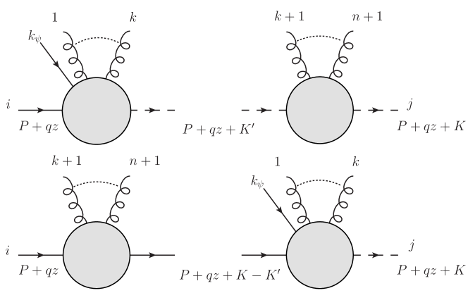
Figure 11: BCFW for the amplitude with 1 gaugino

The amplitude with 1 gaugino and $n+1$ gluons can be computed via BCFW recursion. There are two interesting terms in this recursion. These are shown in the figure 11. By the hypotheses $P(n)$ and $Q(n)$, the first line leads to

$$\left[\sum_{p=1}^{n-k+1}\sum_{q=1}^{k+1}{c^{2}_{a_{1}\ldots a_{p}}T^{(a_{1}}\ldots T^{a_{p})}\over z^{p-2}}{c^{1}_{a_{1}\ldots a_{q}}T^{(a_{1}}\ldots T^{a_{q})}\over z^{q-2}}\right]{1+{\rm O}\left({1\over z}\right)\over 2qz\cdot K^{\prime}},$$

wit $K^{\prime}=k_{\psi}+\sum_{i=1}^{k}k_{i}$. The second line leads to

$$\left[\sum_{p=1}^{n-k+1}\sum_{q=1}^{k+1}{c^{4}_{a_{1}\ldots a_{q}}T^{(a_{1}}\ldots T^{a_{q})}\over z^{q-2}}{c^{3}_{a_{1}\ldots a_{p}}T^{(a_{1}}\ldots T^{a_{p})}\over z^{p-2}}\right]{-1+{\rm O}\left({1\over z}\right)\over 2qz\cdot K^{\prime}}.$$

However, by hypothesis $P(n)$,

$$c^{3}-c^{2}={\rm O}\left({1\over z}\right).$$ (147)

Also,

$$c^{4}-c^{1}={\rm O}\left({1\over z}\right),$$ (148)

since both $c^{4}$ and $c^{1}$ are analytic functions of the external spinors and the external gluon momenta which only differ in the subleading terms in the two cases. Adding the two terms, we now get a commutator and subleading terms

$$\begin{split}&\left[\sum_{p,q}{c^{1}_{a_{1}\ldots a_{p}}c^{2}_{a_{1}\ldots a_{q}}+{\rm O}\left({1\over z}\right)\over z^{p+q-3}}[T^{(a_{1}}\ldots T^{a_{p})},T^{(a_{1}}\ldots T^{a_{q})}]\right]{1\over 2q\cdot K^{\prime}}\\ &+{\rm O}\left({1\over z^{p+q-2}}\right)\{T^{(a_{1}}\ldots T^{a_{p})},T^{(a_{1}}\ldots T^{a_{q})}\}.\end{split}$$

Since the commutator above can be written as a symmetrized product of at most $p+q-1$ generators, we have shown that $P(n)\wedge Q(n)\Rightarrow Q(n+1)$. This completes our proof.

B.2 Explicit Checks

Table 4: Dominant diagrams at large $z$

Scalars	Fermions

We now perform explicit checks of (66) by drawing Feynman diagrams in q-lightcone gauge. As we described in section (5.1), the advantage of this gauge is that it lets us write down all diagrams that contribute to the symmetrized product of generators at some order. In Table 4, we have drawn these diagrams for both scalars and fermions. The diagrams on the first line give us the leading coefficient of $T^{a}$; the diagrams on the second line give us the leading contribution to the symmetrized product of two generators. The diagrams on the third and fourth line give us the leading contribution to the symmetrized product of three generators. We emphasize that the gluon lines shown in these diagrams do not necessarily belong to external gluons. They could as well come come from a gluon propagator that connects to the external gluons through the blobs shown in the diagrams. As in 5.1, we have parametrized the interactions of the matter fields with the gluon lines through background vectors $A_{i}$. These carry momentum $l_{i}$ and to lighten the notation we take the color-index also to be $i$. Also, $K=\sum l_{i}$ and we always keep the decomposition (53) in mind. Our objective here is to verify (66) using explicit calculations in q-lightcone gauge. We put $g=1$ below but keep track of all other factors.

Single Generator

The coefficient $c^{1}$ in (47) is dominated by diagrams that have a single gluon-matter vertex. The first line of Table 4 shows this interaction for both fermions and scalars. The scalar diagram evaluates to

$${\cal M}^{s}=\left(2iqz\cdot A_{1}+{\rm O}\left({1}\right)\right)T^{1}_{ji}.$$ (149)

The fermionic amplitude is (reading the Feynman diagram in the first line of Table 4 against the line)

$${\cal M}^{f}=iT^{1}_{ji}\bar{\lambda}_{\dot{\alpha}}A_{1}^{\dot{\alpha}\beta}\lambda_{\beta}z=2iqz\cdot A_{1}T^{1}_{ji}+{\rm O}\left({1}\right).$$ (150)

Note, that the $\bar{\lambda}$ on the left, comes from the cut-line on the right. In principle, we could have chosen to decompose the momentum here into different spinors than the choice we made for the cut-line on the left. We would then not have got an answer that matched with the scalar answer. This is the relevance of condition (53).

Symmetrized Product of 2 Generators

With two gauge-boson matter vertices we can get a term with a symmetrized product of two generators. The scalar and fermion amplitudes are dominated by the diagrams on the second line of Table 4 and we find

$${\cal M}^{s}=iA_{1}\cdot A_{2}\{T^{1},T^{2}\}_{ji}.$$ (151)

Note, that the q-lightcone gauge implies that it must be possible to write $A_{1}$ and $A_{2}$ as

$$A_{1}^{\alpha\dot{\alpha}}=\lambda^{\alpha}\bar{a}_{1}^{\dot{\alpha}}+\bar{\lambda}^{\dot{\alpha}}a_{1}^{\alpha}.$$ (152)

where $a_{1}$ and $\bar{a}_{1}$ are some spinors. Summing over the two arrangements of the gluon lines, we find the large z fermionic contribution

$${\mathcal{M}}_{f}=-i(\bar{\lambda}_{\dot{\alpha}}\bar{a}_{1}^{\dot{\alpha}}\lambda^{\beta}(l_{1})_{\beta\dot{\gamma}}\bar{\lambda}^{\dot{\gamma}}a_{2}^{\nu}\lambda_{\nu}){T^{1}T^{2}\over q\cdot l_{1}z}+1\leftrightarrow 2+{\rm O}\left({1\over z}\right).$$ (153)

Note the advantage of the q-lightcone gauge here. the momentum running between lines 1 and 2 is actually $P+q+l_{1}$. However, the $q$-lightcone gauge tells us that if we decided to contract $A_{1}$ and $A_{2}$ with the $q$ in the center, then we would pick up the subleading pieces $\bar{\lambda}_{s}^{2}$ and $\lambda_{s}^{1}$ on the right and the left. This would give us an overall power of ${1\over z}$. The contribution to the symmetric term is obtained by adding the coefficients of the two color-factors above. This is

$$\begin{split}{\mathcal{M}}_{f}&=-i{\{T^{1},T^{2}\}\over 2}\left(\left\langle a^{1},\lambda\right\rangle[\bar{\lambda},\bar{a}^{2}]+\left\langle a^{2},\lambda\right\rangle[\bar{\lambda},\bar{a}^{1}]+{\rm O}\left({1\over z}\right)\right)+\ldots\\ &=\left(iA_{1}\cdot A_{2}+{\rm O}\left({1\over z}\right)\right)\{T^{1},T^{2}\}+\ldots\end{split}$$ (154)

where the $\ldots$ denote terms proportional to $[T^{1},T^{2}]$. So the contribution to the second order symmetrized product from scalars and fermions is again the same.

Note that while the contribution to the symmetric product is the same as that of the scalar, the contribution to the commutator term is not. However, the commutator is effectively a single-generator term this contribution is subleading to the leading single-generator term that we evaluated above which is ${\rm O}\left({z}\right)$.

Symmetrized Product of 3 Generators

We now turn to the diagram with 3 external lines. We consider three gluon lines carrying momenta $l_{i}$. This is somewhat more complicated than above. For the scalar, summing the diagram in line 3 of table 4 and the other permutations of the gluon lines, we get

$$\begin{split}{\mathcal{M}}^{s}&=i^{3}{\left((2P+l^{3})\cdot A_{3}\right)\left(A_{1}\cdot A_{2}\right)\over qz\cdot l^{3}}\{T^{2},T^{1}\}T^{3}+i^{3}{\left((2(P+l^{1}+l^{2})+l^{3})\cdot A_{3}\right)\left(A_{1}\cdot A_{2}\right)\over qz\cdot(P+l^{1}+l^{2})}T^{3}\{T^{1},T^{2}\}\\ &+{\rm 2~{}permutations}+{\rm O}\left({1\over z^{2}}\right)\\ &=\left[{2i\over z}{(l_{1}+l_{2})\cdot A_{3}\over q\cdot l_{3}}+{\rm 2~{}permutations}+{\rm O}\left({1\over z^{2}}\right)\right]T^{(1}T^{2}T^{3)}+\ldots\end{split}$$ (155)

On the other hand defining $\chi_{\alpha\dot{\alpha}}=(\lambda z+\lambda_{s}^{1})_{\alpha}(\bar{\lambda}+{\bar{\lambda}_{s}^{2}\over z})_{\dot{\alpha}}$, the fermionic amplitude can be conveniently written as a trace

$$\begin{split}{\mathcal{M}}_{f}&=i^{5}{{\rm Tr}\left[(\chi\cdot\sigma)(A_{3}\cdot\bar{\sigma})\left((P+qz+l^{1}+l^{2})\cdot\sigma\right)(A_{2}\cdot\bar{\sigma})\left((P+qz+l^{1})\cdot\sigma\right)(A_{1}\cdot\bar{\sigma})\right]\over(2qz\cdot l^{1})(2qz\cdot(l^{1}+l^{2}))}\,T^{3}T^{2}T^{1}\\ &+{\rm 6~{}permutations}+{\rm O}\left({1\over z^{2}}\right).\end{split}$$ (156)

While the $\sigma$ matrix algebra is somewhat complicated here, it is quite easy to check with the help of a computer that the contribution to the completely symmetrized third order product is the same to leading order

$${\mathcal{M}}^{f}-{\mathcal{M}}^{s}={\rm O}\left({1\over z^{2}}\right)T^{(1}T^{2}T^{3)}+\ldots$$ (157)

4 External Lines

At first sight, the diagram on the last lines of Table 4 might seem confusing. This seems to give a term with 4 generators but only comes with a ${\rm O}\left({1\over z}\right)$. However, there are six other diagrams that contribute to the same 4^th order symmetrized product that comes from this diagram. In particular, the diagram shown gives a contribution

$$i^{3}\left[{(A_{1}\cdot A_{2})(A_{3}\cdot A_{4})\over 2z}\right]\left[{\{T^{3},T^{4}\}\{T^{1},T^{2}\}\over q\cdot(l_{1}+l_{2})}\right]+{\rm O}\left({1\over z^{2}}\right).$$ (158)

However, there is another diagram for which the first bracket is the same but the term in the second bracket is different. This arises from permuting the 4-pt vertices in the figure. Adding these terms, we find that the contribution to the amplitude is given by

$$\begin{split}i^{3}\left[{(A_{1}\cdot A_{2})(A_{3}\cdot A_{4})\over 2z}\right]\times\left[{\{T^{3}T^{4}\}\{T^{1}T^{2}\}\over q\cdot(l_{1}+l_{2})}+{\{T^{1}T^{2}\}\{T^{3}T^{4}\}\over q\cdot(l_{3}+l_{4})}\right]+{\rm O}\left({1\over z^{2}}\right).\end{split}$$ (159)

We now note that

$$q\cdot(l_{1}+l_{2}+l_{3}+l_{4})=0,$$ (160)

because both the BCFW-extended legs are null. This means that the term in (159) simplifies to

$$\left[{(A_{1}\cdot A_{2})(A_{3}\cdot A_{4})\over z}\right]{\left[\{T^{3}T^{4}\},\{T^{1}T^{2}\}\right]\over(q\cdot(l_{1}+l_{2}))}+{\rm O}\left({1\over z^{2}}\right).$$ (161)

However the term above can be written as a symmetrized trace of up to 3 generators. As we expect, this comes with a factor of ${\rm O}\left({1\over z}\right)$. The proof that the fermionic term shown on the last line of Table 4 gives the same leading contribution to the completely symmetric part of the amplitude is very similar to the proof given for the case with 2-external lines and we will not repeat it here.

Note that (158) does give a ${\rm O}\left({1\over z^{2}}\right)$ contribution to the 4^th order symmetrized product even after we permute the gluon lines. We also need to consider another set of diagrams involving one 4-pt vertex and 2 3-pt vertices. The sum of these two sets of diagrams matches the leading fermionic contribution to the 4^th order product. In a very similar spirit, one can check that the diagrams with 5 and 6 external lines that give a contribution to the 4^th order symmetrized product are the same, to leading order, for fermions and scalars.

Appendix C Feynman Diagrams vs BCFW: An Explicit Tree Amplitude

In this appendix, we perform a simple calculation that shows, how our new recursion relations work in detail. We will consider a $2\rightarrow 2$ scattering processes in a ${\mathcal{N}}=1$ gauge theory without matter.

We take our particles to have momenta $k_{i}$ (marked as ingoing) with a spinor decomposition $k_{i}^{\alpha\dot{\alpha}}=\lambda_{i}^{\alpha}\bar{\lambda}_{i}^{\dot{\alpha}}$, with $i=1\ldots 4$. We take $b_{1}=b_{2}=0,b_{3}=b_{4}=1$. We will label the first two Grassmann parameters by $\xi^{1},\xi^{2}$, and the third and fourth by $\eta 1,\eta^{2}$. Our analysis here is valid for a general gauge group with structure constants $f^{abc}$.

In this example, we will show — through a direct evaluation of Feynman diagrams — that this scattering amplitude has the right behavior when the first two momenta are BCFW extended.

We perform the BCFW extension

$$\lambda_{1}\rightarrow\lambda_{1}+z\lambda_{2},\>\bar{\lambda}_{2}\rightarrow\bar{\lambda}_{2}-z\bar{\lambda}_{1},\>\xi_{1}\rightarrow\xi_{1}+z\xi_{2},$$ (162)

and expand the scattering amplitude in a power series in the Grassmann parameters. Keeping only the non-vanishing terms, this leads to

$$\begin{split}&{\mathcal{A}}^{\mathrm{t}}(\xi^{1}(z),\xi^{2},\eta^{1},\eta^{2})={\mathcal{A}}^{\mathrm{t}}(g^{-},g^{-},g^{+},g^{+})+\xi^{1}\eta^{2}{\mathcal{A}}^{\mathrm{t}}(f^{-},g^{-},g^{+},f^{+})+\xi^{1}\eta^{1}{\mathcal{A}}^{\mathrm{t}}(f^{-},g^{-},f^{+},g^{+})\\ &+\xi^{1}\xi^{2}\eta^{1}\eta^{2}{\mathcal{A}}^{\mathrm{t}}(f^{-},f^{-},f^{+},f^{+})+\xi^{2}\eta^{2}\left[{\mathcal{A}}^{\mathrm{t}}(g^{-},f^{-},g^{+},f^{+})+z{\mathcal{A}}^{\mathrm{t}}(f^{-},g^{-},g^{+},f^{+})\right]\\ &+\xi^{2}\eta^{1}\left[{\mathcal{A}}^{\mathrm{t}}(g^{-},f^{-},f^{+},g^{+})+z{\mathcal{A}}^{\mathrm{t}}(f^{-},g^{-},f^{+},g^{+})\right],\end{split}$$ (163)

where $f^{\pm}$ denotes a fermion with helicity ${\pm}{1\over 2}$ and $g^{\pm}$ denotes a gluon with helicity $\pm 1$. Every amplitude above has an implicit dependence on $z$ through the spinors which have been extended in (162). We see that for ${\mathcal{A}}^{\rm t}(\xi^{1},\xi^{2},\eta^{1},\eta^{2})$ to vanish in the large $z$ limit non-trivial cancellations are required. For example ${\mathcal{A}}^{\rm t}(g^{-},f^{-},f^{+},g^{+})+z{\mathcal{A}}^{\rm t}(f^{-},g^{-},f^{+},g^{+})$ should vanish as z goes to infinity. We now show that this is indeed the case.

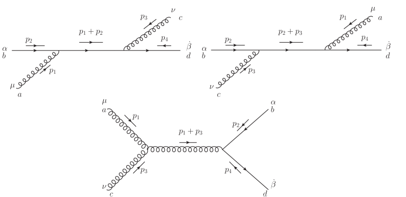
Figure 12: Feynman diagrams: 2 fermions to 2 gluons

The amplitude for ${\mathcal{A}}^{\rm t}(g^{-},f^{-},f^{+},g^{+})$ receives contributions from three diagrams which are shown in figure 12 and may be evaluated to obtain the expression

$$\left.{\mathcal{A}}^{\rm t}(g^{-},f^{-},g^{+},f^{+})\right|_{z=0}=\frac{2\langle\lambda_{2},\lambda_{1}\rangle^{2}}{\langle\lambda_{3},\lambda_{1}\rangle\langle\lambda_{2},\lambda_{4}\rangle}\left(\frac{\langle\lambda_{4},\lambda_{1}\rangle}{\langle\lambda_{4},\lambda_{3}\rangle}f^{cde}f^{aeb}-\frac{\langle\lambda_{2},\lambda_{1}\rangle}{\langle\lambda_{2},\lambda_{3}\rangle}f^{ade}f^{ceb}\right).$$ (164)

The scattering amplitude ${\mathcal{A}}^{\rm t}(f^{-},g^{-},g^{+},f^{+})$ may be obtained from the above expression by interchanging the indices a and b and the labels 1 and 2.

$$\left.{\mathcal{A}}^{\rm t}(f^{-},g^{-},g^{+},f^{+})\right|_{z=0}=\frac{2\langle\lambda_{2},\lambda_{1}\rangle^{2}}{\langle\lambda_{3},\lambda_{2}\rangle\langle\lambda_{1},\lambda_{4}\rangle}\left(\frac{\langle\lambda_{4},\lambda_{2}\rangle}{\langle\lambda_{4},\lambda_{3}\rangle}f^{cde}f^{bea}-\frac{\langle\lambda_{1},\lambda_{2}\rangle}{\langle\lambda_{1},\lambda_{3}\rangle}f^{bde}f^{cea}\right).$$ (165)

The four-fermion scattering amplitude receives contributions from the two Feynman diagrams shown in 13.

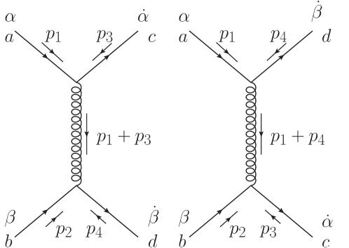
Figure 13: Feynman diagrams for 4 fermion scattering

These diagrams lead to

$$\left.{\mathcal{A}}^{\rm t}(f^{-},f^{-},f^{+},f^{+})\right|_{z=0}=2f^{cae}f^{dbe}\frac{\langle\lambda_{1},\lambda_{2}\rangle^{2}}{\langle\lambda_{1},\lambda_{3}\rangle\langle\lambda_{4},\lambda_{2}\rangle}-2f^{dae}f^{cbe}\frac{\langle\lambda_{1},\lambda_{2}\rangle^{2}}{\langle\lambda_{1},\lambda_{4}\rangle\langle\lambda_{3},\lambda_{2}\rangle}.$$ (166)

We now BCFW extend these expressions, to obtain, in the limit of $z$ approaching infinity

$${\mathcal{A}}^{\rm t}(g^{-},f^{-},g^{+},f^{+})\rightarrow\frac{2\langle\lambda_{2},\lambda_{1}\rangle^{2}}{z\langle\lambda_{3},\lambda_{2}\rangle\langle\lambda_{2},\lambda_{4}\rangle}\left(\frac{z\langle\lambda_{4},\lambda_{2}\rangle}{\langle\lambda_{4},\lambda_{3}\rangle}f^{cde}f^{aeb}-\frac{\langle\lambda_{2},\lambda_{1}\rangle}{\langle\lambda_{2},\lambda_{3}\rangle}f^{ade}f^{ceb}\right),$$ (167)

and

$${\mathcal{A}}^{\rm t}(f^{-},g^{-},g^{+},f^{+})\rightarrow\frac{2\langle\lambda_{2},\lambda_{1}\rangle^{2}}{z\langle\lambda_{3},\lambda_{2}\rangle\langle\lambda_{2},\lambda_{4}\rangle}\left(\frac{\langle\lambda_{4},\lambda_{2}\rangle}{\langle\lambda_{4},\lambda_{3}\rangle}f^{cde}f^{bea}-\frac{\langle\lambda_{1},\lambda_{2}\rangle}{z\langle\lambda_{2},\lambda_{3}\rangle}f^{bde}f^{cea}\right).$$ (168)

Hence we have, in the limit of $z$ approaching infinity

$$\begin{split}&\lim_{z\rightarrow\infty}{\mathcal{A}}^{\rm t}(g^{-},f^{-},g^{+},f^{+})+z{\mathcal{A}}^{\rm t}(f^{-},g^{-},g^{+},f^{+})\\ &=\frac{2\langle\lambda_{2},\lambda_{1}\rangle^{2}}{z\langle\lambda_{3},\lambda_{2}\rangle\langle\lambda_{2},\lambda_{4}\rangle}\left(\frac{\langle\lambda_{4},\lambda_{2}\rangle}{\lambda_{4},\lambda_{3}}f^{cde}\left(f^{aeb}+f^{bea}\right)\right)\\ &=0.\end{split}$$ (169)

The other nontrivial cancellation, between ${\mathcal{A}}^{\rm t}(g^{-},f^{-},f^{+},g^{+})$ and ${\mathcal{A}}^{\rm t}(f^{-},g^{-},f^{+},g^{+})$ can be seen from the above by switching the labels c and d, and 3 and 4. Evidently, the amplitude ${\mathcal{A}}^{\rm t}(f^{-},f^{-},f^{+},f^{+})$ also dies off as ${\rm O}\left({1\over z}\right)$ for large $z$. This proves our result.

References

- [1] S. J. Parke and T. R. Taylor, An Amplitude for Gluon Scattering, Phys. Rev. Lett. 56 (1986) 2459.
- [2] R. Britto, F. Cachazo, and B. Feng, New recursion relations for tree amplitudes of gluons, Nucl. Phys. B715 (2005) 499–522, [hep-th/0412308].
- [3] R. Britto, F. Cachazo, B. Feng, and E. Witten, Direct proof of tree-level recursion relation in Yang- Mills theory, Phys. Rev. Lett. 94 (2005) 181602, [hep-th/0501052].
- [4] A. Brandhuber, P. Heslop, and G. Travaglini, A note on dual superconformal symmetry of the N=4 super Yang-Mills S-matrix, Phys. Rev. D78 (2008) 125005, [arXiv:0807.4097].
- [5] N. Arkani-Hamed, F. Cachazo, and J. Kaplan, What is the Simplest Quantum Field Theory?, arXiv:0808.1446.
- [6] Z. Bern and D. A. Kosower, The Computation of loop amplitudes in gauge theories, Nucl. Phys. B379 (1992) 451–561.
- [7] Z. Bern, L. J. Dixon, and D. A. Kosower, One loop corrections to five gluon amplitudes, Phys. Rev. Lett. 70 (1993) 2677–2680, [hep-ph/9302280].
- [8] Z. Bern, L. J. Dixon, D. C. Dunbar, and D. A. Kosower, One loop n point gauge theory amplitudes, unitarity and collinear limits, Nucl. Phys. B425 (1994) 217–260, [hep-ph/9403226].
- [9] Z. Bern, L. J. Dixon, D. C. Dunbar, and D. A. Kosower, Fusing gauge theory tree amplitudes into loop amplitudes, Nucl. Phys. B435 (1995) 59–101, [hep-ph/9409265].
- [10] Z. Bern and A. G. Morgan, Massive Loop Amplitudes from Unitarity, Nucl. Phys. B467 (1996) 479–509, [hep-ph/9511336].
- [11] Z. Bern, N. E. J. Bjerrum-Bohr, and D. C. Dunbar, Inherited twistor-space structure of gravity loop amplitudes, JHEP 05 (2005) 056, [hep-th/0501137].
- [12] N. E. J. Bjerrum-Bohr, D. C. Dunbar, H. Ita, W. B. Perkins, and K. Risager, The no-triangle hypothesis for N = 8 supergravity, JHEP 12 (2006) 072, [hep-th/0610043].
- [13] N. E. J. Bjerrum-Bohr and P. Vanhove, Absence of Triangles in Maximal Supergravity Amplitudes, JHEP 10 (2008) 006, [arXiv:0805.3682].
- [14] S. Badger, N. E. J. Bjerrum-Bohr, and P. Vanhove, Simplicity in the Structure of QED and Gravity Amplitudes, JHEP 02 (2009) 038, [arXiv:0811.3405].
- [15] I. P. Ennes, C. Lozano, S. G. Naculich, and H. J. Schnitzer, Elliptic models, type IIB orientifolds and the AdS/CFT correspondence, Nucl. Phys. B591 (2000) 195–226, [hep-th/0006140].
- [16] M. Bershadsky and A. Johansen, Large N limit of orbifold field theories, Nucl. Phys. B536 (1998) 141–148, [hep-th/9803249].
- [17] A. Hodges, Eliminating spurious poles from gauge-theoretic amplitudes, arXiv:0905.1473.
- [18] D. Nguyen, M. Spradlin, A. Volovich, and C. Wen, The Tree Formula for MHV Graviton Amplitudes, arXiv:0907.2276.
- [19] N. Arkani-Hamed, F. Cachazo, C. Cheung, and J. Kaplan, A Duality For The S Matrix, arXiv:0907.5418.
- [20] J. Wess and J. Bagger, Supersymmetry and supergravity. Princeton Series in Physics. Princeton University Press, 1992. 259 p.
- [21] L. J. Dixon, Calculating scattering amplitudes efficiently, hep-ph/9601359.
- [22] N. Arkani-Hamed and J. Kaplan, On Tree Amplitudes in Gauge Theory and Gravity, JHEP 04 (2008) 076, [arXiv:0801.2385].
- [23] C. Cheung and D. O’Connell, Amplitudes and Spinor-Helicity in Six Dimensions, arXiv:0902.0981.
- [24] R. H. Boels, Covariant representation theory of the Poincare algebra and some of its extensions, arXiv:0908.0738.
- [25] V. P. Nair, A Current Algebra for some Gauge Theory Amplitudes, Phys. Lett. B214 (1988) 215.
- [26] S. Mandelstam, Light Cone Superspace and the Ultraviolet Finiteness of the N=4 Model, Nucl. Phys. B213 (1983) 149–168.
- [27] C. Cheung, On-Shell Recursion Relations for Generic Theories, arXiv:0808.0504.
- [28] R. Britto, F. Cachazo, and B. Feng, Generalized unitarity and one-loop amplitudes in N = 4 super-Yang-Mills, Nucl. Phys. B725 (2005) 275–305, [hep-th/0412103].
- [29] Z. Bern, L. J. Dixon, and D. A. Kosower, Bootstrapping multi-parton loop amplitudes in QCD, Phys. Rev. D73 (2006) 065013, [hep-ph/0507005].
- [30] C. F. Berger, Z. Bern, L. J. Dixon, D. Forde, and D. A. Kosower, Bootstrapping one-loop QCD amplitudes with general helicities, Phys. Rev. D74 (2006) 036009, [hep-ph/0604195].
- [31] D. Forde, Direct extraction of one-loop integral coefficients, Phys. Rev. D75 (2007) 125019, [arXiv:0704.1835].
- [32] C. F. Berger et. al., An Automated Implementation of On-Shell Methods for One- Loop Amplitudes, Phys. Rev. D78 (2008) 036003, [arXiv:0803.4180].
- [33] S. Raju, The Noncommutative S-Matrix, JHEP 06 (2009) 005, [arXiv:0903.0380].
- [34] G. Chalmers and W. Siegel, Simplifying algebra in Feynman graphs. II: Spinor helicity from the spacecone, Phys. Rev. D59 (1999) 045013, [hep-ph/9801220].
- [35] D. Vaman and Y.-P. Yao, QCD recursion relations from the largest time equation, JHEP 04 (2006) 030, [hep-th/0512031].
- [36] S. Okubo, Modified fourth-order casimir invariants and indices for simple lie algebras, Journal of Mathematical Physics 23 (1982), no. 1 8–20.
- [37] S. Kachru and E. Silverstein, 4d conformal theories and strings on orbifolds, Phys. Rev. Lett. 80 (1998) 4855–4858, [hep-th/9802183].
- [38] J. Erlich and A. Naqvi, Nonperturbative tests of the parent/orbifold correspondence in supersymmetric gauge theories, JHEP 12 (2002) 047, [hep-th/9808026].
- [39] M. Schmaltz, Duality of non-supersymmetric large N gauge theories, Phys. Rev. D59 (1999) 105018, [hep-th/9805218].
- [40] M. J. Duff, Twenty years of the Weyl anomaly, Class. Quant. Grav. 11 (1994) 1387–1404, [hep-th/9308075].
- [41] S. S. Gubser, Einstein manifolds and conformal field theories, Phys. Rev. D59 (1999) 025006, [hep-th/9807164].
- [42] O. Aharony, S. S. Gubser, J. M. Maldacena, H. Ooguri, and Y. Oz, Large N field theories, string theory and gravity, Phys. Rept. 323 (2000) 183–386, [hep-th/9905111].
- [43] J. Park and A. M. Uranga, A note on superconformal N = 2 theories and orientifolds, Nucl. Phys. B542 (1999) 139–156, [hep-th/9808161].
- [44] A. Armoni, M. Shifman, and G. Veneziano, Exact results in non-supersymmetric large N orientifold field theories, Nucl. Phys. B667 (2003) 170–182, [hep-th/0302163].
- [45] S. Okubo and J. Patera, General indices of representations and casimir invariants, Journal of Mathematical Physics 25 (1984), no. 2 219–227.
- [46] S. Okubo and J. Patera, General indices of simple lie algebras and symmetrized product representations, Journal of Mathematical Physics 24 (1983), no. 12 2722–2733.
- [47] S. Okubo, Casimir invariants and vector operators in simple and classical lie algebras, Journal of Mathematical Physics 18 (1977), no. 12 2382–2394.
- [48] T. van Ritbergen, A. N. Schellekens, and J. A. M. Vermaseren, Group theory factors for Feynman diagrams, Int. J. Mod. Phys. A14 (1999) 41–96, [hep-ph/9802376].
- [49] S. Okubo, Quartic Trace Identity for Exceptional Lie Algebras, J. Math. Phys. 20 (1979) 586.
- [50] J. Fuchs and C. Schweigert, Symmetries, Lie algebras and representations. Cambridge University Press New York, NY, USA, 1997.