An anisotropic preconditioning for the Wilson fermion matrix on the lattice

Abstract

A preconditioning for the Wilson fermion matrix on the lattice is defined, which is particularly suited to the case when the temporal lattice spacing is much smaller than the spatial one. Details on the implementation of the scheme are given. The method is tested in numerical studies of QCD on anisotropic lattices.

I Introduction

Anisotropic discretisations Morningstar and Peardon (1997); Umeda et al. (2003); Morrin et al. (2006) have proved an extremely useful tool for determining the energy spectrum of lattice field theories using the Monte Carlo method. Four dimensional Euclidean space-time is discretised with separate grid spacings $a_{s}$ and $a_{t}$ for the spatial dimensions and the temporal direction with $\xi=a_{s}/a_{t}$. The spectrum of the theory is determined by measuring the correlation function between operators on the fields in a Monte Carlo calculation and performing a statistical analysis to determine the rate of decay of these functions. This fall-off is related to the energies of eigenstates of the quantum-mechanical hamiltonian. A fine resolution in the temporal direction is crucial to make an accurate determination of energies, particularly when considering massive or highly excited states. The advantage of the anisotropic lattice is that the rapid rise in numerical effort needed to reduce the lattice spacing is ameliorated by just reducing the spacing in the time direction. The Hadron Spectrum collaboration is currently using these lattice regularisations in a large-scale programme Lin et al. (2009); Edwards et al. (2008); Lin et al. (2007) aiming to measure the QCD spectrum to high precision. The calculations by the collaboration include the full dynamics of the lightest three quark fields and in these investigations, the dominant source of computational overhead is solving the linear system corresponding to quark propagation in a given gauge field background. Quark propagation is described by finding solutions to a lattice representation of the Euclidean-space Dirac equation:

$$(D\!\!\!\!/+m)\psi=\eta,$$ (1)

where $D\!\!\!\!/$ is the Dirac operator in the presence of the gauge fields. The Hadron Spectrum collaboration has used anisotropic lattices with Wilson and Sheikholeslami-Wohlert Sheikholeslami and Wohlert (1985) discretisations of the Dirac operator. These solutions, $\psi$ must be computed during application of the Markov process that generates the ensemble of gauge fields for Monte Carlo importance sampling as well as during the measurement phase. The vector space in which the solution is to be constructed is sufficiently large that direct methods are impractical and instead iterative solvers must be employed. While the anisotropic lattice gives substantial benefits in statistical precision the disadvantage is that the inclusion of a fine discretisation scale; $a_{t}$; increases the condition number of the linear system to be solved. This naturally leads to an increase in the number of iterations needed in the solver. A well-established means of improving efficiency is to precondition the problem.

A quick examination reveals that the dominant terms in the coefficient matrix of the linear system represent the discretisation of the temporal derivative in the Dirac operator. In this work, operators that directly inverts this term are constructed and used to form a preconditioner. Once the means of applying the inverse of the temporal term in the Wilson or SW operator has been defined it is seen that further preconditioning using Schur or ILU factorisation can be applied. To test this idea, the condition numbers of temporally preconditioned operators are computed on several gauge field ensembles. This test uses quenched ensembles since they are substantially easier to generate with a range of different anisotropies than fully dynamical ones, and the issue of determining the parameters in the lattice action needed to give a particular physical anisotropy $\xi$ is greatly simplified. The temporal preconditioned matrices to be inverted have condition numbers approximately twenty times smaller than their unpreconditioned counterparts and about three to four times smaller than the commonly used even-odd lattice Schur preconditioning when the anisotropy ranges from three to six. Taking into account numerical overheads, this translates to cost reductions of around 1.7-2.4. No advantage is found using temporal preconditioning in the isotropic case.

This paper is organized as follows: in section II we set up our notation, and describe in detail the basics of temporal preconditioning and how it may be combined with further even-odd preconditioning. In section III we detail our numerical investigations, including the tuning of our fermion anisotropy parameters and a presentation of condition numbers for various kinds of preconditioning schemes. We sum up and draw our conclusions in section IV.

II Theory

The Wilson fermion matrix and its ${\cal O}(a)$-improved Sheikholeslami-Wohlert (SW) version can be defined on an anisotropic lattice with three coarse spatial directions with spacing $a_{s}$ and a fine temporal spacing $a_{t}$. In practice, the anisotropy is introduced into the simulation by modifying the couplings in the lattice action that weight temporal and spatial components. There relative weights are denoted $\gamma_{g}$ for terms in the gauge action and $\gamma_{f}$ for the fermions. These parameters are tuned carefully to ensure Lorentz invariance is restored in long-distance physics. If these parameters are determined using a perturbative expansion, then at the tree level they are $\gamma_{f}=\gamma_{g}=\xi$. Since practical simulations will be performed close to the continuum limit, this relationship should hold to within approximately $25\%$. Following the notation of Lin et al. (2009), we will denote the tuned values of these parameters as $\gamma^{*}_{g}$ and $\gamma^{*}_{f}$ respectively.

With these definitions, the fermion matrix is defined as the sum of the following terms:

$$M=A+\mu\delta_{x,y}-D_{t}-\frac{1}{\gamma_{f}}D_{s},$$ (2)

with

$$D_{t}=\frac{1-\gamma_{0}}{2}U_{0}(x)\delta_{x+\hat{0},y}+\frac{1+\gamma_{0}}{2}U^{\dagger}_{0}(x-\hat{0})\delta_{x-\hat{0},y},$$ (3)

$$D_{s}=\sum_{i=1}^{3}\left(\frac{1-\gamma_{i}}{2}U_{i}(x)\delta_{x+\hat{i},y}+\frac{1+\gamma_{i}}{2}U^{\dagger}_{i}(x-\hat{i})\delta_{x-\hat{i},y}\right),$$ (4)

where $\gamma_{i}$ for $i=0,1,2,3$ are appropriate spin matrices and $\mu$ is an anisotropic mass term corresponding to bare mass $m_{0}$ defined as $\mu=a_{t}m_{0}+1+\frac{3}{\gamma_{f}}$.

In the case of Wilson fermions, the term $A=0$ while for the SW improved fermion matrix the mass term $\mu$ and the hopping terms $D_{s}$ and $D_{t}$ are unchanged while the corresponding expression for $A$ is

$$A=-\delta_{x,y}\left\{\frac{c_{t}}{2}\sum_{i=1}^{3}\sigma_{i0}F_{i0}(x)+\frac{c_{s}}{2}\sum_{ij}\sigma_{ij}F_{ij}(x)\right\}\ ,$$ (5)

where $\sigma_{ij}=\frac{1}{2}\left[\gamma_{i},\gamma_{j}\right]$ is a commutator of the spin matrices and $F_{ij}(x)$ is the anti-hermitian “clover-leaf” term constructed from the plaquettes in the $i,j$ plane emanating from from site $x$ as defined in Lin et al. (2009) and elsewhere.

The tree level tadpole improvement coefficients $c_{s}$ and $c_{t}$ are defined as

$$c_{s}=\frac{1}{u^{3}_{s}}\frac{1}{\gamma_{f}},\qquad c_{t}=\frac{1}{2u^{2}_{s}u_{t}}\left(\frac{\gamma_{g}}{\gamma_{f}}+\frac{1}{\xi}\right),$$ (6)

where $u_{s}$ is the spatial tadpole factor computed from the spatial plaquettes of our gauge ensembles $U_{ss}$ as

$$u_{s}=\langle\frac{1}{3}U_{ss}\rangle^{\frac{1}{4}},$$ (7)

and we have set $u_{t}=1$. The isotropic case is recovered when one sets $u_{s}=u_{t}$, $\gamma_{g}=\gamma_{f}=1$ and so $c_{s}=c_{t}$ are the same tree level improved tadpole coefficient.

As in the isotropic case, these linear operators act on vectors in an $N_{c}\times N_{\gamma}\times N_{s}$-dimensional space of complex fermion fields, where $N_{c}$ is the number of colors in the gauge group, $N_{\gamma}=4$ is the number of components in a spin-1/2 representation of the group of four-dimensional Euclidean rotations and $N_{s}$ the number of sites on the four-dimensional lattice.

The additional terms in the SW action are all diagonal in the spatial and temporal lattice co-ordinates. With the matrix expressed in this form, the largest terms in $M$ are contained in $A$, $D_{t}$ and $\mu$, and the contribution from terms in $D_{s}$ is smaller by a factor of the (bare fermion) anisotropy. This suggests an efficient preconditioning for this matrix can be constructed if a way of applying the inverse of $A+\mu-D_{t}$ is known. Notice this matrix is block-diagonal in the spatial lattice co-ordinates, so solving this problem requires being able to invert a one-dimensional lattice operator.

II.1 A temporal preconditioner

We now proceed to present the technique of the temporal preconditioning. In the discussion below, we will initially focus on the Wilson case ($A=0$) for simplicity. We will then comment upon the strategies available to deal with the full SW case. We begin by defining temporal spin-projection operators

$$P_{\pm}=\frac{1}{2}(1\pm\gamma_{0}),$$ (8)

and a temporal hopping matrix at every spatial site on the lattice

$$T_{t,t^{\prime}}(\vec{x})=\mu\delta_{t,t^{\prime}}-U_{0}(\vec{x},t)\delta_{t+1,t^{\prime}},\quad t=0\ldots N_{t}-1,$$ (9)

where $N_{t}$ is the number of lattice points in the temporal direction of the lattice. The operator $T$ is gauge covariant with no spin structure. Further, $T$ can have a variety of boundary conditions. We will consider primarily the cases where $T$ is either periodic or anti–periodic where

$$T_{N_{t}-1,N_{t}-1}(\vec{x}) = \mu$$ (10)

$$T_{0,N_{t}-1}(\vec{x}) = \pm U_{0}(\vec{x},N_{t}-1)\ ,$$ (11)

and the sign in Eqn. 11 is positive or negative when the boundary conditions are respectively periodic or anti-periodic.

We now define operators on all spin components,

$$C_{L}^{-1}=P_{+}+P_{-}T\mbox{ and }C_{R}^{-1}=P_{-}+P_{+}T^{\dagger},$$ (12)

where the invertability of these matrices has been assumed. With these definitions, the temporal hopping term can be expressed as

$$\mu-D_{t}=C_{L}^{-1}C_{R}^{-1}\ .$$ (13)

Constructing $C_{L}^{-1}$ and $C_{R}^{-1}$ with the spin-projector structure given above ensures they obey the relation

$$C_{L}^{\dagger-1}=\gamma_{5}C_{R}^{-1}\gamma_{5},$$ (14)

which will allow the construction of a preconditioned matrix that maintains $\gamma_{5}$ hermiticity. Eqn. 13 now shows how $C_{L}$ and $C_{R}$ will make a useful preconditioner for the Wilson fermion matrix on the anisotropic lattice. The fermion matrix can be written as

$$M=C_{L}^{-1}C_{L}MC_{R}C_{R}^{-1}=C_{L}^{-1}\tilde{M}C_{R}^{-1},$$ (15)

with $\tilde{M}=C_{L}MC_{R}$. For Wilson fermions,

$$\tilde{M}=I-\frac{1}{\gamma_{f}}C_{L}D_{s}C_{R},$$ (16)

and the preconditioned matrix is equal to the identity plus terms proportional to $1/\gamma_{f}$ only.

The operation of $\tilde{M}$ on a fermion field requires the operation of $C_{L}=(P_{+}+P_{-}T)^{-1}$. Since $P_{+}$ and $P_{-}$ define orthogonal projectors, this inverse can be re-written as $C_{L}=P_{+}+P_{-}T^{-1}$ and the application of $C_{L}$ is reduced to finding the inverse of $T$. If the lattice fields had Dirichlet boundary conditions, $T$ (a lattice representation of the forward-difference operator) could be inverted easily by back-substitution, starting at the open boundary. Most lattice calculations use periodic or anti-periodic boundary conditions however and so back-substitution is insufficient. The Sherman-Morrison-Woodbury (SMW) Sherman and Morrison (1949, 1950); Woodbury (1950) formula provides a simple means of inverting a matrix that differs in a small number of elements from another matrix whose inverse is computationally cheap to apply. The forward difference operator with periodic boundary data, $T$ can be written in terms of the difference operator with open boundaries, $T_{0}$ and a correction term:

$$T=T_{0}+VW^{\dagger},$$ (17)

with

$$[T_{0}]_{t,t^{\prime}}(\vec{x})=\left\{\begin{array}[]{ll}\mu\delta_{t,t^{\prime}}-U_{0}(\vec{x},t)\delta_{t+1,t^{\prime}}&\mbox{ if }\;\;t=0..N_{t}-2\\ \mu\delta_{t,t^{\prime}}&\mbox{ if }\;\;t=N_{t}-1,\end{array}\right.$$ (18)

and $V$ and $W$ are $N_{c}N_{t}\times N_{c}$ column matrices where the only non-zero entries are in either the first or last sites:

$$V_{t}(\vec{x})=-U_{0}(\vec{x},t)\delta_{t,N_{t}-1},$$ (19)

and

$$W_{t}(\vec{x})=\delta_{t,0}.$$ (20)

Since $T$, $T_{0}$, $V$ and $X$ are defined on each spatial site $\vec{x}$, we will suppress the spatial index in subsequent discussion except where it may be needed for clarity. With these definitions, $VW^{\dagger}$ is a rank $N_{c}$ correction that adds the effects of the boundary condition back in to the open-boundary-data operator. The SMW formula then gives an expression for the inverse of $T$ defined in Eqn. 17. Defining $X=T_{0}^{-1}V$ yields

$$T^{-1}=T_{0}^{-1}-X(I+W^{\dagger}X)^{-1}W^{\dagger}.$$ (21)

All that remains to be evaluated is $(I+W^{\dagger}X)^{-1}$ but note that this is a small (rank $N_{c}$) matrix at each spatial site whose inverse is straightforwardly computed. In practice, the algorithm proceeds as follows:

1. Prior to use, the preconditioner is initialized. On each spatial site $\vec{x}$, the expression

   1. $X=T_{0}^{-1}V$ is computed by back-substitution and

   2. $\Lambda=(I+W^{\dagger}X)^{-1}$ is subsequently computed.

   All these results are stored. $\Lambda$ requires storage of just $N_{c}\times N_{c}$ complex numbers per spatial site, while $X$ requires $N_{c}\times N_{c}N_{t}$. This is smaller storage requirement than a single fermion field. Also, we note that one can immediately compute $X\Lambda$ at this point which also requires storage of $N_{c}\times N_{c}N_{t}$ per spatial site but which may overwrite the original $X$.

2. Given a particular right-hand side $\eta$, computing $\psi=T^{-1}\eta$ requires first evaluating

   1. $\chi=T_{0}^{-1}\eta$ by back-substitution, then

   2. $q=\Lambda W^{\dagger}\chi$. Note that $W^{\dagger}\chi$ is just the $N_{c}$-component vector on time-slice $t=0$ of vector $\chi$ and so evaluation of $W^{\dagger}\chi$ is computationally trivial. Finally, the solution is formed:

   3. $\psi=\chi-Xq$

The back substitution process for $X$ can formally be carried out analytically. For the case of $T$ one has:

$$X(\vec{x},N_{t}-1) = -\frac{1}{\mu}U_{t}(\vec{x},N_{t}-1),$$ (22)

$$X(\vec{x},t) = -\frac{1}{\mu^{N_{t}-t}}\prod_{j=N_{t}-t}^{N_{t}-1}U_{t}(\vec{x},j)\ \mbox{for $0\leq t<N_{t}-1$},$$ (23)

and successive terms in $X$ are suppressed by powers of the mass term $\mu$, and the matrix product forms a series which for $X(\vec{x},0)$ is the Polyakov loop. In principle; for large enough $N_{t}$; one could find some $k$ such that for $0\leq t<k$ one has $X(\vec{x},i)\approx 0$ numerically, and one may then save some numerical effort by just setting those values of $X(\vec{x},t)=0$ and not evaluating matrix products using them but setting them to zero also. Since the link matrices in the components of $X$ are $SU(3)$ one knows that their product is also $SU(3)$ and hence one can find the norm of $X(\vec{x},i)$ as

$$||X(\vec{x},t)||=\sqrt{3}\mu^{-\left(N_{t}-t\right)},$$ (24)

where the factor of $\sqrt{3}$ comes from the $SU(3)$ nature of the link matrices. We will refer to the cutting off the computation of $X(\vec{x},t)$ for sufficiently small values of $t$ as the cutoff trick. Caution should be used however to ensure there is no impact in the precision of final result.

The inverse of $T^{\dagger}$, required for the operation of $C_{R}$ is formed in the same way, using appropriate redefinitions of $X,W$ and $V$ and with forward-substitution solves. We note that in step 1(b) above, only an $N_{c}\times N_{c}$ complex matrix needs to be inverted per site. The cutoff trick also works, but now the terms are least suppressed at $t=0$ (open end of the forward substitution) and most suppressed at $t=N_{t}-1$, building up to the Hermitean conjugate of the Polyakov loop for $X(\vec{x},N_{t}-1)$, and the $N_{t}-t$ term in eqn. 24 needs to be replaced with $t$.

Let us now comment on the case for SW fermions. Proceeding as above, the entire procedure is valid, but the preconditioned matrix changes to:

$$\tilde{M}=C_{L}MC_{R}=I+C_{L}\left(A-\frac{1}{\gamma_{f}}D_{s}\right)C_{R}\ .$$ (25)

It then becomes tempting to extend the definition of $C^{-1}_{L}$ and $C^{-1}_{R}$ in such a way that

$$A+\mu-D_{t}=C^{-1}_{L}C^{-1}_{R},$$ (26)

so that the preconditioned matrix would maintain its original $I-\frac{1}{\gamma_{f}}C_{L}D_{s}C_{R}$ form, even in the case of a general, non-zero SW term, ı.e. $A\neq 0$. The practical difficulty with this approach is that the $\sigma_{\mu\nu}$ terms in $A$ couple all spin components and the forward and backward difference operators in $D_{t}$ cease to be directly separable. Correspondingly the construction of suitable $C_{L}$ and $C_{R}$ terms would require the inversion of a block-tridiagonal matrix, with $N_{\gamma}N_{c}\times N_{\gamma}N_{c}$ sized blocks rather than just $N_{c}\times N_{c}$. Further, the back/forward substitutions fill-in these blocks destroying the site wise block-diagonal structure of the SW matrix and so, the inversions of the diagonal blocks would need dense inversions of the full $N_{\gamma}N_{c}$ dimensional sub-blocks. We will refer to this approach as full SW temporal preconditioning. The details of this approach are discussed in the appendix.

Nonetheless, even if one just uses the same $C_{L}$ and $C_{R}$ as for the Wilson action and suffers the contamination from the SW term in the preconditioned matrix $\tilde{M}$ in eq. (25), it can be seen that the $D_{t}$ term is still inverted, and that the $D_{s}$ terms are suppressed by a factor of $\frac{1}{\gamma_{f}}$. Hence one can expect that this form of preconditioning is still more effective than using the unpreconditioned operator. In what follows we will refer to this approach of using the $C_{L}$ and $C_{R}$ preconditioners from the case of the Wilson fermion matrix to preconditione the SW operator, as partial SW temporal preconditioning.

II.2 Combining the temporal preconditioner with other schemes

The usual isotropic Wilson and SW operators are efficiently preconditioned by considering a Schur decomposition after first ordering lattice sites according to their four-dimensional co-ordinate parity, $p_{4}(x)=(-1)^{x_{0}+x_{1}+x_{2}+x_{3}}$. One has

$$M=\left(\begin{array}[]{cc}M^{ee}&M^{eo}\\ M^{oe}&M^{oo}\end{array}\right)=\left(\begin{array}[]{cc}I^{ee}&0\\ M^{oe}[M^{ee}]^{-1}&I^{oo}\end{array}\right)\left(\begin{array}[]{cc}M^{ee}&0\\ 0&M^{oo}-M^{oe}[M^{ee}]^{-1}M^{eo}\end{array}\right)\left(\begin{array}[]{cc}I^{ee}&[M^{ee}]^{-1}M^{eo}\\ 0&M^{oo}\end{array}\right),$$ (27)

with $M^{ee(oo)}=A^{ee(oo)}+\mu$, and $M^{eo}=-D^{eo}_{w}$, $D^{eo}_{w}=\frac{1}{\gamma_{f}}D_{s}+D_{t}$ being the 4-dimensional Wilson Dslash operator, and the Schur preconditioned matrix is

$$\tilde{M}=\left(\begin{array}[]{cc}M^{ee}&0\\ 0&M^{oo}-M^{oe}[M^{ee}]^{-1}M^{eo}\end{array}\right)\ .$$ (28)

This kind of Schur preconditioning with a $p_{4}$ ordering, is the standard even-odd preconditioning method in use for Wilson and SW fermions, and we shall refer to it as 4D-Schur preconditioning from now on.

This idea can be combined with the temporal preconditioner with a small modification; instead of ordering lattice sites by a four-dimensional parity, a three-dimensional equivalent is used, $p_{3}(x)=(-1)^{x_{1}+x_{2}+x_{3}}$. The preconditioned matrix $\tilde{M}$ retains its form in terms of $M^{ee(oo)}$ and $M^{eo(oe)}$, however these now change their meaning slightly, since with this ordering, the operators $A$ and $D_{t}$ connect lattice sites with the same $p_{3}$ while the spatial hopping matrix couples sites with opposite $p_{3}$. and

$$M^{ee(oo)}=A^{ee(oo)}+\mu-D_{t}^{ee(oo)}\ ,\qquad M^{eo(oe)}=-\frac{1}{\gamma_{f}}D^{eo(oe)}_{s}.$$ (29)

For the Wilson action, the inverse of the block matrix, $M^{ee}=\mu-D_{t}^{ee}$ is formed using the method described in the previous section. For full temporal preconditioning in the clover case, one would need to form the inverse of $M^{ee}=A^{ee}+\mu-D_{t}^{ee}$ the difficulties with which have already been discussed, and we can refer to the result as temporal preconditioning combined with 3D-Schur preconditioning. Alternatively, one can proceed with partial preconditioning for the Clover case, using the $p_{3}$ ordering preconditioner appropriate for the Wilson action. In this case we can refer to the result as temporal preconditioning combined with 3D incomplete lower-upper (ILU) preconditioning.

First, we define the action of the left temporal preconditioner on the even 3-parity sub-lattice to be $C^{e}_{L}$ and define correspondingly the right preconditioner and both their odd sub-lattice counterparts to be $C^{e}_{R},C^{o}_{L},C^{o}_{R}$. We also introduce the notation that for some generic term $K$ the corresponding term $\bar{K}$ is defined as $\bar{K}=C_{L}KC_{R}$. Hence,

$$\bar{D}_{s}^{eo}=C_{L}^{e}D_{s}^{eo}C_{R}^{o}.$$ (30)

To keep the discussion below general, we will also define the operator

$$\bar{Q}=C_{L}\left(A+\mu-D_{t}\right)C_{R}\ .$$ (31)

In the case of Wilson fermions, $A=0$ and so $\bar{Q}=I$. For SW fermions with full SW preconditioning one also has $\bar{Q}=1$ while with partial SW preconditioning,

$$\bar{Q}=1+C_{L}AC_{R}=1+\bar{A}\ .$$ (32)

$\bar{Q}$ is diagonal in terms of $p_{3}$ even-odd indices, and we may refer to its even-even (odd-odd) sub blocks $\bar{Q}^{ee(oo)}$ using $C^{e(o)}_{L}$, $C^{e(o)}$ and $A^{ee(oo)}$ as needed.

With these expressions, the even-odd preconditioners for the Wilson matrix become

$$S_{L}=\left(\begin{array}[]{cc}C_{L}^{e}&0\\ \frac{1}{\gamma_{f}}\bar{D}_{s}^{oe}C_{L}^{e}&C_{L}^{o}\end{array}\right)\mbox{ and }S_{R}=\left(\begin{array}[]{cc}C_{R}^{e}&\frac{1}{\gamma_{f}}C_{R}^{e}\bar{D}_{s}^{eo}\\ 0&C_{R}^{o}\end{array}\right),$$ (33)

which gives

$$\tilde{M}_{3}=S_{L}MS_{R}=\left(\begin{array}[]{cc}\bar{Q}^{ee}&-\frac{1}{\gamma_{f}}\left[1-\bar{Q}^{ee}\right]\bar{D}_{s}^{eo}\\ -\frac{1}{\gamma_{f}}\bar{D}_{s}^{oe}\left[1-\bar{Q}^{ee}\right]&\bar{Q}^{oo}-\frac{1}{\gamma^{2}_{f}}\bar{D}_{s}^{oe}\left[2-\bar{Q}^{ee}\right]\bar{D}_{s}^{eo}\end{array}\right).$$ (34)

If $\bar{Q}=1$, as is the case of Wilson fermions or Clover fermions with full temporal preconditioning, this matrix reduces to

$$\tilde{M}_{3}=\left(\begin{array}[]{cc}1&0\\ 0&1-\frac{1}{\gamma^{2}_{f}}\bar{D}_{s}^{oe}\bar{D}_{s}^{eo}\end{array}\right),$$ (35)

so that the preconditioned matrix differs from the identity only by terms proportional to $\frac{1}{\gamma^{2}_{f}}$. In the case of partial SW preconditioning, where $\bar{Q}=1+\bar{A}$, the preconditioned matrix is

$$\tilde{M}_{3}=\left(\begin{array}[]{cc}1+\bar{A}^{ee}&\frac{1}{\gamma_{f}}\bar{A}^{ee}\bar{D}_{s}^{eo}\\ \frac{1}{\gamma_{f}}\bar{D}_{s}^{oe}\bar{A}^{ee}&1+\bar{A}^{oo}-\frac{1}{\gamma^{2}_{f}}\bar{D}_{s}^{oe}\left[1-\bar{A}^{ee}\right]\bar{D}_{s}^{eo}\end{array}\right).$$ (36)

We can see from eq. 36 that in contrast to full preconditioning in eq. 35, we now have non–zero off diagonal elements (in even-odd space) that are only suppressed by $\gamma_{f}$. Further the diagonal elements contain components proportional to $a_{t}$ in the Clover terms $\bar{A}$. These terms can counter potential suppression by $\gamma_{f}^{2}$ in the odd-odd checkerboarded term of $\tilde{M}_{3}$.

To complete this discussion, we note that effective use of the preconditioner requires the inverses $S^{-1}_{L}$ and $S^{-1}_{R}$ to be applied so the solutions with the unpreconditioned matrices may be obtained. Using the definitions of $C^{-1}_{L(R)}$ restricted to the even and odd sites respectively we have

$$S^{-1}_{L}=\left(\begin{array}[]{cc}\left(C_{L}^{e}\right)^{-1}&-\frac{1}{\gamma_{f}}\bar{D}^{eo}\left(C_{L}^{o}\right)^{-1}\\ 0&\left(C_{L}^{o}\right)^{-1}\end{array}\right)\mbox{ and }S^{-1}_{R}=\left(\begin{array}[]{cc}\left(C_{R}^{e}\right)^{-1}&0\\ -\frac{1}{\gamma_{f}}\left(C_{R}^{e}\right)^{-1}\bar{D}_{s}^{eo}&\left(C_{R}^{o}\right)^{-1}\end{array}\right)\ .$$ (37)

II.3 Numerical cost of ILU Scheme

We consider the partial temporally preconditioned scheme, combined with ILU even-odd preconditioning to be potentially the most attractive, since it is simple in terms of implementation and is equivalent to the full 3D Schur preconditioned scheme in the case of Wilson fermions. However, applying the preconditioners does incur some numerical overhead. The overhead depends to some degree on details of the implementation of the method. We will consider two implementations below.

First we consider the naive implementation of the method, with no gauge fixing and in spinor basis where $\gamma_{0}$ is not diagonal. This could be the case in a general code, using a chiral spin-basis such as the Chroma software system Edwards and Joo (2005). Neglecting the cost of preparing the sources and recovering the solutions (using $S^{-1}_{L}$ and $S^{-1}_{R}$) we can compare costs of the usual 4D Schur preconditioning and the partially temporally preconditioned ILU scheme, which we will denote as $\mathcal{C}(\tilde{M}_{\rm 4DSchur})$ and $\mathcal{C}(\tilde{M}_{\rm ILU})$ respectively, by counting the floating point operations (FLOPs) in the respective preconditioned linear operators.

Relegating the actual counting of FLOPs to appendix .2, we merely state here that the ratio of floating point costs:

$$R=\frac{\mathcal{C}(\tilde{M}_{\rm ILU})}{\mathcal{C}(\tilde{M}_{\rm 4DSchur})},$$ (38)

is

$$R^{W}=\frac{3432N_{t}-576}{2668N_{t}}\approx 1.286-\frac{0.216}{N_{t}},$$ (39)

for Wilson fermions, and

$$R^{C}=\frac{6012N_{t}-1152}{3732N_{t}}\approx 1.611-\frac{0.309}{N_{t}},$$ (40)

for Clover fermions respectively, resulting typically in about a 29% overhead for Wilson, and 61% overhead for Clover from the ILU scheme in terms of FLOPs as compared to the standard 4D Schur even-odd scheme. This must be matched by the gain in terms of condition number from the preconditioner for it to remain competitive.

Concurrent with writing this paper, some clever optimization techniques were brought to our attention by the authors of Clark et al. ; Barros et al. (2008) arising from work with General Purpose Graphics Processing Units (GPGPUs). These techniques save both memory bandwidth and FLOPs. The first technique we consider is to fix the gauge prior to the inversion proess, to the Axial gauge (temporal gauge). The effect of this operation is that all the links that are not on the temporal boundary are transformed to the unit matrix: $U_{0}(\vec{x},t)=1$ for $t=0\ldots N_{t}-2$. This can save floating point operations in the back(forward) substitutions with $T_{0}$, where in each step one can save an SU(3) matrix-color vector multiply. Further, one can save on memory requirements since the block vector $X$ is simplified to

$$X(\vec{x},t)=\frac{1}{\mu^{N_{t}-t}}U_{0}(\vec{x},N_{t}-1),$$ (41)

with the other terms in the partial Polyakov loops now being the identity. Correspondingly, instead of storing all of $X$, one can easily compute any component of it from the boundary link matrix which one stores anyway. Fixing to the axial gauge is a straightforward operation which can be amortized over either one and especially over several solves.

The second trick that can prove useful is to employ the Dirac-Pauli spin basis in which $\gamma_{0}$ is diagonal. This simplifies the projector operators $P_{+}$ and $P_{-}$ so that they select the top or bottom two spin components of four spinors respectively. This can save FLOPs on spinor reconstuction (which now no longer needs to be done in the time direction) but also when one has a sum of the form

$$S=P_{+}\psi+P_{-}\chi,$$ (42)

one has no arithmetic to perform, since the spin components filtered by the projectors can be written directly into the correct components of $S$ without requiring any addition. We enumerate in explicit detail the savings from these two implementation techniques in appendix .3. It is shown there that employing both of these techniques can save roughly 22-25% in terms of FLOPs over the naive implementation.

When compared to the 4D-Schur preconditioned scheme, which also benefits from these improvements, we find that the techniques result in relative overhead ratios of:

$$R^{W}=\frac{2664N_{t}-48}{2044N_{t}}\approx 1.30-\frac{0.023}{N_{t}},$$ (43)

for Wilson fermions, and

$$R^{C}=\frac{4476N_{t}-96}{3108N_{t}}\approx 1.440-\frac{0.031}{N_{t}},$$ (44)

for Clover fermions. In particular, the relative overhead for the Clover operator appears to be substantially reduced compared to the naive implementation (44% as opposed to the previous 61%). The foregoing discussion does not make use of the cutoff trick, which can be used to further reduce the floating point costs of the preconditioned operators as discussed earlier.

III Numerical Investigation

III.1 Strategy and Choice of Parameters

Wishing to investigate the efficacy of the preconditioning strategies as functions of both lattice anisotropy and quark mass in as realistic a setting as possible, we have opted to measure the condition numbers of the various operators in three quenched ensembles. These ensembles were chosen to have target (renormalized) anisotropies of $\xi=1.0$, $\xi=3.0$ and $\xi=6.0$ respectively, thus ranging from the fully isotropic to the highly anisotropic. We picked a wide range of quark masses, to give pion masses in the range of about $450$ MeV to $750$ MeV. We note that this necessitated us tuning the fermion anisotropies $\gamma_{f}$ so as to make the renormalized anisotropies $\xi$ (as fixed by the pion dispersion relation) the same as our target anisotropies $\xi$, a subject we will discuss in more detail further on.

During our study, we have opted to keep the physical temporal extent of the lattice fixed in the time direction. This approach means that as we increased the anisotropy, we likewise increased the number of lattice points in the time direction. We have used $N_{t}=16$, $N_{t}=48$, $N_{t}=96$ for the anisotropies of $\xi=1.0$, $\xi=3$ and $\xi=6$ respectively. This increase of the temporal resolution may have an effect on the condition numbers of our operators. We felt however, that this is typically the approach one would use in a real calculation, rather than keeping the temporal extent fixed, and that we should absorb this effect in our efficiency estimates, in order to give a realistic measure of the performance of the preconditioning.

III.2 Code and Computers

We coded the temporal preconditioned Wilson-Clover operators, in the Chroma Edwards and Joo (2005) software system. We implemented both 3D ILU and 3D Schur even-odd preconditionings in space, in combination with the temporal preconditioning. In the case of the 3D Schur even-odd preconditioning, we used an inner Conjugate Gradients solve, to invert $M^{ee}$ in the Schur complement. We also used the unpreconditioned and 4D Schur Even-Odd preconditioned operators already present in the Chroma suite to measure reference results. Our implementations used the naive implementation technique discussed in sec. II.3. In order to tune the fermion anisotropies, we carried out some hadron spectroscopy calculations, in particular the measurement of the pseudoscalar correlation functions at various momenta. In order to measure the condition numbers of the square operators, we used the Ritz-minimization technique of Bunk (1997). Both these sets of measurements are standard within the Chroma distribution. Fitting of our spectroscopy results used the so called 4H code developed by UKQCD. Our calculations were carried out on the Jefferson Lab 6n and 7n clusters.

III.3 Selecting the Gauge Action Parameters

We chose our isotropic reference case, to be a quenched dataset with the Wilson gauge action at $\beta=6.0$ as it is well known in the literature to have a lattice spacing of $0.1$fm Michael and Shanahan (1996). In the anisotropic case using $\beta=6.1$ has approximately the same spatial lattice spacing at $\xi=3$ and $\xi=6$ Klassen (1998). We chose the bare gauge anisotropies from the formula suggested by Klassen (1998). Our gauge production parameters are summarized in Table 1.

$\xi^{T}$	$\beta$	$V$ ($N_{s}^{3}\times N_{t}$)	$\gamma^{*}_{g}$	$u_{s}$
$1$	$6.0$	$16^{3}\times 16$	$1$	$0.8780$
$1$	$6.0$	$16^{3}\times 48(\dagger)$	$1$	$0.8780$
$3$	$6.1$	$16^{3}\times 48$	$2.464$	$0.8279$
$6$	$6.1$	$16^{3}\times 96$	$4.7172$	$0.8195$

Table 1: Parameters of the Quenched Ensembles used in this study. In the first column $\xi^{T}$ refers to the desired target anisotropies, with the final bare gauge anisotropies $\gamma^{*}_{g}$ being shown in the 4th column. Apart from ($\dagger$) the temporal extent grows from $N_{t}=16$ with the anisotropy. ($\dagger$) was used merely for checking the pion mass at the isotropic parameter set since the $N_{t}=16$ case was too short for measuring the pion mass. We also show our measurements for the spatial tadpole coefficient $u_{s}$.

III.4 Tuning the Fermion Parameters

In this study, we have opted to use Clover fermions, with tree-level tadpole improved clover coefficients as defined in Ref. 6. In the anisotropic cases, we needed to tune the fermion anisotropy as well as our quark masses to fall within our desired range.

Our tuning exercise then comprised of choosing trial values, of $\gamma_{f}$ for a selection of values for $m_{0}$, and computing the pion dispersion relations for each $(m_{0},\gamma_{f})$ pair. Since anisotropic tuning is not the main subject of our paper, we were content to do this very roughly and were satisfied by a renormalized anisotropy within 10% of our target. To compute the dispersion relation, we extracted the ground state energies ($E_{o}$) of the pion for several initial momenta $\vec{p}$, by fitting the pion correlation function:

$$C(t,\vec{p})=\sum_{\vec{x}}e^{i\vec{x}.\vec{p}}\langle\mathcal{O}^{\dagger}(\vec{x},t)\mathcal{O}(\vec{0},0)\rangle\ \stackrel{{\scriptstyle{t\rightarrow\infty}}}{{\rightarrow}}\ 2Ae^{-E_{0}\frac{N_{t}}{2}}\cosh\left(E_{0}(\frac{N_{t}}{2}-t)\right),$$ (45)

where $\mathcal{O}$ is a suitable pion interpolating operator:

$$\mathcal{O}(\vec{x},t)=\bar{\psi}(\vec{x},t)\Gamma\psi(\vec{x},t).$$ (46)

We used spatial momenta ranging in magnitude from $|\vec{p}^{2}|=0$ to $|\vec{p}^{2}|=\left(\frac{3}{2\pi N_{s}}\right)^{2}$. We averaged the correlation function over the momenta that resulted in equal values of $|\vec{p}^{2}|$. We used the interpolating operator $\Gamma=\gamma_{5}$ for the zero momentum fits, whereas for the finite momentum fits we used $\Gamma=\gamma_{4}\gamma_{5}$ as we found the signal to be cleaner.

Once $E_{0}$ was determined for all values of $|\vec{p}|^{2}$, we fitted them to the dispersion relation formula:

$$E^{2}=\frac{1}{\xi^{2}}p^{2}+\hat{m}^{2},$$ (47)

where $\hat{m}=E_{0}(|\vec{p}|^{2}=0)$, by a straight line fit, to extract $\xi$. To compute our estimate for the pion mass, we then computed the mass in units of the spatial lattice spacing: $a_{s}m_{\rm latt}=\xi\hat{m}$, and then converted this number to physical units assuming $a_{s}=0.1$fm.

The correlation functions themselves were constructed using gaussian gauge invariant source smearing Allton et al. (1993), and stout link smearing Morningstar and Peardon (2004). No smearing was performed at the sink. Our tuning calculations were carried out using 40-100 configurations for each $(m_{0},\gamma_{f})$ pair. We used the bootstrap method to estimate our errors on the masses and fitted anisotropies with 200 bootstrap samples in each case. When estimating the physical pion mass, we added the bootstrap errors on $\xi$ and $\hat{m}$ in quadrature, rather than under the bootstrap. The results of our tuning are shown in table 2 wherein we show the fitted fermion anisotropies, and our estimates of the mass of the pion.

$\xi^{T}$	$m_{0}$	$\gamma^{*}_{f}$	$\xi$	$E(\vec{p}=0)$	$m_{\pi}$ (MeV)	# configs used
1	-0.359	1	1	0.383(3)	766(6)	100
1	-0.379	1	1	0.296(2)	597(4)	100
1	-0.392	1	1	0.225(2)	450(4)	59
3	-0.13	2.95	3.06(4)	0.105(2)	641(15)	46
3	-0.132	2.96	3.08(4)	0.097(1)	597(12)	46
3	-0.135	2.96	3.03(4)	0.082(2)	498(15)	46
6	-0.058	5.43	5.99(10)	0.0578(9)	693(16)	50
6	-0.061	5.63	5.96(10)	0.042(1)	504(17)	41

Table 2: At each of our target anisotropies $\xi^{T}$, we show the bare values of $m_{0}$, our tuned bare fermion anisotropy $\gamma^{*}_{f}$, and the resulting measured renormalized anisotropies $\xi$ as determined from the pion dispersion relation. We also show the resulting pion masses in lattice units ($E(\vec{p}=0)$) and in physical units ($m_{\pi}$). The $\xi=1.0$ results were determined on the $16^{3}\times 48$ lattice.

III.5 Results

With the tuned fermion parameters in hand, we computed the condition numbers for the various kinds of preconditionings in our three quenched ensembles. We did not make use of the cutoff trick in our temporally preconditioned operators. This time in the isotropic case, we used the $N_{t}=16$ ensemble, since we did not need long time extents for fitting. Specifically we computed condition numbers for the unpreconditioned (Unprec), and the 4D Schur even-odd preconditioned operator (4D Schur) to use as a standard to compare against, as well as the temporally preconditioned operators combined with both 3D ILU even-odd preconditioning (TPrec+ILU) and Schur style preconditioning in 3-dimensions (Tprec+3D Schur). We used 19 configurations from each ensemble to measure the condition numbers.

In figure 1 we show how the condition number of the unpreconditioned operator varies with pion (quark) mass and anisotropy. We can see, as one would expect, that the condition numbers increase with decreasing pion (quark) mass as well as with increasing anisotropy.

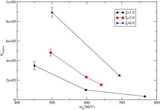
Figure 1: The condition numbers of the unpreconditioned clover operator against the measured pion mass, for all three of our anisotropy values: $\xi=1.0$ (black circles), $\xi=3.0$ (red squares) and $\xi=6.0$ (blue diamonds).

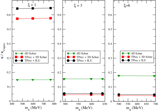
Figure 2: Ratios of the condition numbers of the preconditioned operators to the unpreconditioned operator at the same mass and anisotropy (lower is better conditioned). The 3 panes are for anisotropies of $\xi=1$ (left), $\xi=3$ (middle), $\xi=6$ (right). The colors are 4D Schur preconditioning (green triangles), temporal preconditioning + 3D ILU (black circles), temporal preconditioning + 3D Schur preconditioning (red squares)

In figure 2 we plot the ratios of the condition numbers of the preconditioned operators to the condition number of the unpreconditioned operator. We separate the results into three graphs for the three values of $\xi$ used. Separation in terms of $\gamma_{f}$ is not practical since for different masses, one can have different values of $\gamma_{f}$ for the same renormalized anisotropy $\xi$. The ratios give a nice clean signal, as it appears that from configuration to configuration, the ratios do not fluctuate very much (although the condition numbers themselves do). Hence the average of the ratios is very stable.

First we can see in the leftmost graph of fig. 2, that in the isotropic case, the greatest gain comes from the 4D Schur preconditioning, whose condition number is about 15% of the unpreconditioned (Unprec.) case. Some gain over the unpreconditioned case can still be achieved using temporal preconditioning combined with either 3D Schur (TPrec + 3D Schur) or partial temporal preconditioning with ILU in 3D (TPrec + ILU). However the temporally preconditioned cases are not as efficacious as the 4D Schur preconditioning in the isotropic case. Looking at the middle and rightmost graphs of fig. 2 we see that in the anisotropic cases, the temporally preconditioned operators fare much better, with condition numbers that are around 4% - 6% of the upreconditioned one.

We note that the mass dependence in these ratios appears to be very mild, for a given value of $\xi$. Also with the temporal preconditioning we see an improvement in the condition number ratios as $\xi$ is increased. This is presumably due to the suppression factors of $\frac{1}{\gamma_{f}}$ and $\frac{1}{\gamma^{2}_{f}}$ in the temporally preconditioned operators. We expect this is because of the clover term in the preconditioner which has components in both the spatial and temporal directions, and the temporal components will counteract the suppression factors $\gamma_{f}$ and $\gamma_{f}^{2}$ to some degree. It is however encouraging to see that the partial preconditioning combined with 3D-ILU even-odd preconditioning in space is nearly as good as the 3D Schur preconditioned case. This suggests that not dealing with the clover term in the preconditioner is not in fact catastrophic. This is welcome news as the 3D-ILU preconditioning is considerably simpler to implement and involves fewer FLOPs than the fully preconditioned 3D-Schur approach.

We replot the condition number data in figure 3, this time plotting the ratio of the condition number of the 4D Schur operator to those of the temporally preconditioned operators, to see if we gain in condition with respect to the “standard preconditioning”. The ratios are are defined as

$$\frac{\kappa_{\mbox{4D Schur}}}{\kappa_{\mbox{TPrec.+ILU}}},\ \mbox{and}\frac{\kappa_{\mbox{4D Schur}}}{\kappa_{\mbox{TPrec.+3D Schur}}}\ .$$ (48)

and hence values larger than one indicates that the temporally preconditioned operator is better conditioned than the Schur4D, whereas values less than one indicate that the Schur4D is better conditioned.

We see, as before, in the leftmost graph of fig. 3, that in the isotropic case, neither of the temporal preconditioned approaches can beat the 4D Schur preconditioned approach. The condition numbers of the temporally preconditiond operators are about 4 times the Schur 4D case. Looking at the middle and rightmost graphs, one sees that the TPrec.+ILU preconditinong gives a decrease in the condition number of about a factor 2.8-3.8 (depending on $\xi$), while the TPrec+3D Schur preconditioning gives a decrease of a factor of about 3.3-4.4 compared to the standard 4D Schur even odd preconditioning (again depending on $\xi$).

At this point, we should recall that the numerical overhead of the ILU style preconditioning is between 44%-61% depending on implementation. Using the most conservative overhead of 61%, this gives an overall gain in total cost for this scheme, compared to the 4D Schur case, of $2.8/1.61-3.8/1.61$ which equates to between $1.74-2.36$ for anisotropies of $\xi=3-6$. With the most optimistic overhead estimate (44%) these gains can grow to $1.94-2.64$.

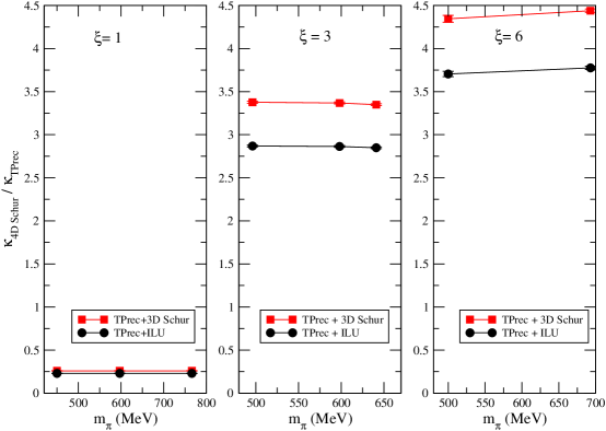
Figure 3: Ratios of the condition numbers of the 4D Schur even-odd preconditioned operator to the two temporally preconditioned cases (higher is better conditioned). The 3 panes are for anisotropies of $\xi=1$ (left), $\xi=3$ (middle), $\xi=6$ (right). The colors are 4D Schur/TPrec + ILU (black circles), and 4D Schur/TPrec + 3D Schur (red squares)

IV Conclusions

We have demonstrated the technique of temporal preconditioning for anisotropic discretizations of the Wilson and SW Dirac operator in lattice QCD. We discussed the implementation of the technique in an efficient manner, and its combination with further even-odd preconditioning techniques, in particular the 3D-ILU and 3D Schur even-odd approaches.

In the case of Wilson fermions, the 3D-ILU and 3D-Schur approaches are in fact identical and we have shown that the only terms in the preconditioned matrix that differ from the identity are suppressed by two powers of the anisotropy, $\xi^{2}$. For SW fermions, the presence of the clover term complicates the implementation since there are explicit terms that are diagonal in spatial indices and that connect the null spaces of the forward and backward projectors. The 3D-ILU approach remains straightforward, however, the resulting preconditioned matrix has non-zero off diagonal elements, which are only suppressed by factors of $\xi$ rather than $\xi^{2}$.

We implemented the method in Chroma, a general code base for lattice QCD. We have also considered optimization techniques suggested from work in the realm of GPGPUs. The appendix shows that the number of floating point operations in the temporally preconditioned operator with ILU even-odd preconditioning is about 30% and 61% higher than the corresponding 4D Schur preconditioned operator for the Wilson and SW operators respectively in the most generic case. Specialized implementation can reduce floating point the overhad of the Clover action to about 44%. These costs may further be ameliorated as needed through judicious use of the cutoff trick. We have not used the cutoff trick in the numerical results of this paper.

We have carried out numerical tests in a variety of quenched ensembles, both isotropic and anisotropic to investigate the efficacy of the techniques discussed, using Wilson-Clover fermions at a range of quark masses.

Our chief conclusion is that the technique works well for anisotropic cases. In our studies, with anisotropies of $\xi=3$ and $\xi=6$, the temporally preconditioned Clover operator with ILU preconditioning had condition numbers between a factor of about 2.8-3.3 times smaller than the usual 4D Schur preconditioned case, whereas the temporally preconditioned operator with 3D Schur even-odd preconditioning had condition numbers that were about 3.3-4.4 times smaller than the usual 4D Schur preconditioned case. Combined with the various overhead estimates, this gives the temporally preconditioned, ILU preconditioned clover operator a cost advantage of a factor of $1.74-2.36$ over the more standard 4D Schur preconditioned approach depending on implementation. The 4D Schur preconditioner, however, appeared to be the best conditioned in the isotropic case.

Due to the decreases in condition number observed using the temporal preconditioned methods, it becomes attractive to extend the preconditioning scheme to Hybrid Molecular Dynamics-Monte Carlo algorithm such as Hybrid Monte Carlo Duane et al. (1987). New terms will arise in the Hamiltonian, due to the determinants of the preconditioning matrices. We leave the full discussion of these ramifications to a future publication.

V Acknowledgements

This work was done using the Chroma software suite Edwards and Joo (2005) on clusters at Jefferson Laboratory using time awarded under the USQCD Initiative. MP was supported by Science Foundation Ireland under research grants 04/BRG/P0266 and 07/RFP/PHYF168. MP is grateful for the generous hospitality of the theory center at TJNAF during which time some of this research was carried out. We would like to thank Mike Clark and Ron Babich for insightful discussions and pointing out the utility of the Dirac basis and the Axial gauge to this technique. Authored by Jefferson Science Associates, LLC under U.S. DOE Contract No. DE-AC05-06OR23177. The U.S. Government retains a non-exclusive, paid-up, irrevocable, world-wide license to publish or reproduce this manuscript for U.S. Government purposes.

.1 Appendix – Full Preconditioning with Clover

In this appendix, we consider the question of how to deal with the inversion of the term $\left(A+\mu-D_{t}\right)$, in the case of full temporal preconditioning.

We begin with

$$A(\vec{x},t)+\mu-D_{t}(\vec{x},t)=A(\vec{x},t)+\mu-P_{-}U_{t}(\vec{x},t)\delta_{\vec{x},t+1;\vec{x},t^{\prime}}-P_{+}U^{\dagger}_{t}(\vec{x},t-1)\delta_{\vec{x},t-1;\vec{x},t}$$ (49)

Inverting $A+\mu-D_{t}$ can be done with a single step Woodbury procedure:

$$A+\mu-D_{t}=T_{0}+VW^{\dagger}$$ (50)

where

$$V=\left(\begin{array}[]{c}-U^{\dagger}(\vec{x},N_{t}-1)P_{+}\\ 0\\ 0\\ \vdots\\ 0\\ -U(\vec{x},N_{t}-1)P_{-}\end{array}\right)\quad\mbox{,}\quad W^{\dagger}=\left(P_{-},0,0,0,\ldots P_{+}\right)$$ (51)

With the tridiagonal matrix $T_{0}$ is now, supressing space indices:

$$T_{0}=\left(\begin{array}[]{ccccc}A(0)+\mu&-U(0)P_{-}&0&\ldots&0\\ -U^{\dagger}(0)P_{+}&A(1)+\mu&-U(1)P_{-}&0&\ldots\\ 0&\ddots&\ddots&\ddots&\vdots\\ \vdots&&-U^{\dagger}(N_{t}-3)P_{+}&A(N_{t}-2)+\mu&-U(N_{t}-2)P_{-}\\ 0&0&\vdots&-U^{\dagger}(N_{t}-2)P_{+}&A(N_{t}-1)+\mu\end{array}\right)$$ (52)

This matrix, while easy to apply, is not immediately straighforward to invert, because of its projector structure. In our numerical work, to gauge the efficacy of this approach, we used an inner conjugate gradients algorithm to invert this matrix.

.2 Floating Point Operation count for ILU Scheme

Let us recount the the number of floating point operations needed to apply the usual 4D Schur preconditioned operator:

$$\tilde{M}_{{\rm 4DSchur}}=A^{oo}-\frac{1}{4}D^{oe}\left(A^{-1}\right)^{ee}D^{eo}$$ (53)

where the mass term has been absorbed into the diagonal part of $A$ and $D^{oe}$ denotes the 4D Hopping matrix. The parameters $\gamma_{f}$ have been absorbed into a rescaling of the gauge links. We will use the notation $\mathcal{C}(Q)$ do denote the floating point cost of some generic term $Q$. Applying the $A^{oo}$ term and $A^{ee}$ both require 522 FLOPs per site, on $V/2$ sites (single checkerboard) each, giving $\mathcal{C}(A^{oo})=\mathcal{C}(A^{ee})=522(V/2)$ FLOPs

The $D^{oe}$ and $D^{eo}$ terms require 1320 FLOPs each per site on $V/2$ sites (single checkerboard) each. This number is arrived at by considering the spin projection operators as having no floating point operations, since only sign flips and exchanges of real and imaginary components are involved. Each $SU(3)$ matrix-vector (matvec) operation requires $66$ FLOPs, corresponding to three inner products between the three rows of the matrix, and the column vector. Each inner product involves 3 complex multiplies (6 FLOPs each) and 2 complex adds (2 FLOPs each), or $3\times 6+2\times 2=22$ FLOPs, giving a total of $3\times 22=66$ for the three inner products in the complete matvec operation.

Spin reconstuction (recons) takes $12$ FLOPs per site, coming from a single complex add for each of 2 spin-color components (6 complex-adds in total); again, not counting sign flips and real complex component interchanges. Finally, $24$ FLOPs are required to sum two (now reconstructed) 4 spinors (sumvec4) to evaluate the sum over directions (4 spin-color components, so 12 complex components in total, with 2 FLOPs per component).

In $N_{d}$ dimensions

$$\mathcal{C}(D^{oe})=2N_{d}(N^{*}_{\gamma}{\rm matvec}+{\rm recons})+{\rm sumvec4}\times(2N_{d}-1)$$ (54)

where the factor of $2N_{d}$ comes from doing forward and backward projections and reconstructions in $N_{d}$ dimensions, and $N^{*}_{\gamma}$ is the number of spin components left after spin projection. So, in 4-dimensions, with $N_{\gamma}=4$ we have $N_{d}=4,N^{*}_{\gamma}=2$ and one has:

$$\mathcal{C}(D^{oe})=8(2\times 66+12)+24\times 7=1320\ {\rm FLOPs}$$ (55)

Correspondingly, per site the 4D Schur Operator takes up

$$\mathcal{C}(\tilde{M}_{\rm 4DSchur})=2\times\left(1320+522\right)+48=3732\ {\rm FLOPs}$$ (56)

where the last factor of $48$ comes from the AXPY operation to apply the factor of $\frac{1}{4}$ and subtracting the two terms from each other. Hence, applying the operator costs $3732(V/2)$ FLOPs in total, which it is convenient to re-express as $3732N_{t}(V_{s}/2)$, with $N_{t}$ the extent of the time direction, and $V_{s}$ being the number of spatial coordinates per timeslice.

Let us now consider the ILU preconditioned operator

$$\tilde{M}_{\rm ILU}=\left(\begin{array}[]{cc}1+\bar{A}^{ee}&\bar{A}^{ee}\bar{D}^{eo}_{s}\\ \bar{D}^{oe}\bar{A}^{ee}&1+\bar{A}^{oo}-\bar{D}^{oe}_{s}\left[1-\bar{A}^{ee}\right]\bar{D}^{eo}_{s}\end{array}\right)$$ (57)

where we have absorbed the factors of $\xi$ into the $\bar{D}$ terms. Applying $\tilde{M}_{\rm ILU}$ to some vector $\psi$, to result in $\chi=\tilde{M}_{\rm ILU}\psi$ implies that

$$\chi_{e} = \psi_{e}+\bar{A}^{ee}\left(\bar{D}^{eo}\psi_{o}+\psi_{e}\right)$$ (58)

$$\chi_{o} = \psi_{o}+\bar{A}^{oo}\psi_{o}+\bar{D}^{oe}\left\{\bar{A}^{ee}\left[\bar{D}^{eo}\psi_{o}+\psi_{e}\right]-\bar{D}^{eo}\psi_{o}\right\}$$ (59)

and one can reuse several terms between $\chi_{e}$ and $\chi_{o}$. Thus $\tilde{M}_{\rm ILU}$ can be efficiently applied by computing in sequence:

$$\chi_{e} = \psi_{e}$$ (60)

$$\chi_{o} = \psi_{o}$$ (61)

$$t_{1} = \bar{D}^{eo}\psi_{o}$$ (62)

$$t_{2} = \bar{A}^{ee}\left(t_{1}+\psi_{e}\right)$$ (63)

$$\chi_{e} = \chi_{e}+t_{2}$$ (64)

$$\chi_{o} = \chi_{o}+\bar{A}^{oo}\psi_{o}+\bar{D}^{oe}\left(t_{2}-t_{1}\right)$$ (65)

and apart from 5 vector additions, we need to apply $\bar{A}$ and $\bar{D}$ twice each (once per checkerboard). Since $\bar{A}=C_{L}AC_{R}$ and $\bar{D}=C_{L}DC_{R}$ we have

$$\mathcal{C}(\tilde{M}_{\rm ILU})=5\times 24\times(V/2)+2\left[\mathcal{C}(\bar{D}_{s})+\mathcal{C}(\bar{A})\right]=120(V/2)+2\left[2\mathcal{C}(C_{L})+2\mathcal{C}(C_{R})+\mathcal{C}(A)+\mathcal{C}(D_{s})\right]$$ (66)

where the $5\times 24\times(V/2)$ term is to account for the 5 vector adds, each on a single checkerboard.

We still have $\mathcal{C}(A)=522$ per site and by substituting $N_{d}=3$ into the discussion for $\mathcal{C}(D)$ one finds that applications of the 3D $D_{s}$ operator cost 984 FLOPs per site. The preconditioners $C_{L}$ and $C_{R}$ have the same cost each namely $\mathcal{C}(C)$ and so

$$\mathcal{C}(\tilde{M}_{\rm ILU})=120(V/2)+2\left[4\mathcal{C}(C)+\mathcal{C}(A)+\mathcal{C}(D_{s})\right]=120(V/2)+8\mathcal{C}(C)+(2\times 522+2\times 984)(V/2)=8\mathcal{C}(C)+3132(V/2)$$ (67)

Applying $C$ requires a back (forward) subsitution for each spatial site of the appropriate checkerboard. We consider the backsubsitution here, but the working is similar (and the FLOP count is identical) for the forward substitution. The back subsitution needs to be performed on only 2 spin color components, after spin projections with either $1+\gamma_{0}$ or $1-\gamma_{0}$ for $C_{L}$ or $C_{R}$, followed by an appropriate reconstruction. After the backsubsitution the Woodbury procedure involves for each spatial site, working with length $N_{t}$ block vectors, a matrix multiplication by the a pre-computed $SU(3)$ matrix, and an $SU(3)$ subtraction. As usual we do not count any floating point operations for the projection part of the spin projection steps. This gives

$$\mathcal{C}(C)=N^{*}_{\gamma}\left[(V_{S}/2)\left(\mathcal{C}(B)+\mathcal{C}(W)\right)\right]+(V/2)(12+48)$$ (68)

where $V_{s}$ denotes the number of spatial sites, $\mathcal{C}(B)$ denotes the cost for the back substitution, $\mathcal{C}(W)$ denotes the rest of the Woodbury process, the $12(V/2)$ FLOPs come from the spin reconstruction on one chekerboard and the $48(V/2)$ FLOPs come from adding the $P_{+}$ and $P_{-}$ terms in $C_{L}$ and $C_{R}$ ; one vector addition costing 24 FLOPs and an overall scaling by $\frac{1}{2}$ to normalize the projectors costing another 24 FLOPs.

We now need to consider the backsubstution on a single spin color component: The first step is just a scaling by the diagonal $\psi_{N_{t}-1}=\frac{1}{\mu}\chi_{N_{t}-1}$ or 6 FLOPs. Then there follow $N_{t}-1$ steps of $\psi_{i}=\frac{1}{\mu}\left[\chi_{i}-U_{i}\psi_{i+1}\right]$, each one comprised of an $SU(3)$ matrix vector multiply (66 FLOPs) and a subtraction and a scaling by $\mu$ (6 FLOPs each). In total:

$$\mathcal{C}(B)=6+\left(N_{t}-1\right)\left(66+6+6\right)=78N_{t}-72\ {\rm FLOPs}$$ (69)

The remainder of the Woodbury procedure involves computing the $X\Lambda W^{\dagger}$ term. This can be achieved by precomputing $X\Lambda W^{\dagger}$ for each value of $t$ at initialization, and then this process costs only $N_{t}$ matrix vector operations (66FLOPs each), and finally we need to subtract the result of this matrix multiply from the result of the back/forward substitution (6 FLOPs) for each value of $N_{t}$ and so

$$\mathcal{C}(W)=(66+6)N_{t}=72N_{t}\ {\rm FLOPs}$$ (70)

and

$$\mathcal{C}(C) = N^{*}_{\gamma}(V_{s}/2)\left[78N_{t}-72+72N_{t}\right]+(V/2)\left[12+48\right]$$

$$= N^{*}_{\gamma}(V_{s}/2)\left[150N_{t}-72\right]+60(V/2)$$

$$= (V_{s}/2)\left(300N_{t}-144\right)+60N_{t}(V_{s}/2)$$

$$= (V_{s}/2)\left(360N_{t}-144\right)\ {\rm FLOPs}$$

where we have used $V_{s}V_{t}=V$, and $N^{*}_{\gamma}=2$ so

$$\mathcal{C}(\tilde{M}_{\rm ILU}) = 8\mathcal{C}(C)+3132(V/2)$$ (71)

$$= 8(V_{s}/2)\left(360N_{t}-144\right)+3132N_{t}(V_{s}/2)$$

$$= (V_{s}/2)\left(2880N_{t}-1152\right)+3132N_{t}(V_{s}/2)$$

$$= \left(6012N_{t}-1152\right)(V_{s}/2)\ {\rm FLOPs}$$

Comparing the costs of the two preconditioned operators we have for Clover fermions

$$R=\frac{\mathcal{C}(\tilde{M}_{\rm ILU})}{\mathcal{C}(\tilde{M}_{\rm 4DSchur})}=\frac{6012N_{t}-1152}{3732N_{t}}\approx 1.611-\frac{0.309}{N_{t}}$$ (72)

and so we consider two limiting cases: in the first instance when $N_{t}=1$ we have $R=1.302$ to 3 decimal places (d.p.) and when $N_{t}$ is sufficiently large that the term involving it is negligible we have $R=1.611$ to 3 d.p. In a typical case, when $N_{t}=128-256$ one has $R\approx 1.61$ to 2 d.p.

Similarly we can consider the case for just Wilson fermions. In this case

$$\tilde{M}_{{\rm 4DSchur}}=\mu-\frac{1}{4\mu}D^{oe}D^{eo}$$ (73)

and the cost is

$$\mathcal{C}(\tilde{M}_{{\rm 4DSchur}})=(48+2\times 1320)N_{t}(V_{s}/2)=2668N_{t}(V_{s}/2)\ {\rm FLOPs}$$ (74)

where the $48$FLOPS comes from the subtraction, and scaling (AXPY) operation.

The temporally preconditioned scheme needs only the evaluation of

$$\tilde{M}_{{\rm ILU}}=I-\bar{D}^{oe}_{s}\bar{D}^{eo}$$ (75)

and so the cost in flops is:

$$\mathcal{C}(\tilde{M}_{\rm ILU}) = 24(V/2)+4\mathcal{C}(C)+2\mathcal{C}(D_{s})$$ (76)

$$= 24N_{t}(V_{s}/2)+4(V_{s}/2)\left(360N_{t}-144\right)+2\times 984N_{t}(V_{s}/2)$$

$$= (V_{s}/2)\left(24N_{t}+1440N_{t}-576+1968N_{t}\right)$$

$$= (V_{s}/2)\left(3432N_{t}-576\right)\ {\rm FLOPs}$$

and we have

$$R=\frac{3432N_{t}-576}{2668N_{t}}\approx 1.286-0.216\frac{1}{N_{t}}$$ (77)

giving $R$ in the range of $R\approx 1.07-1.286$.

Use of the cutoff trick removes the multiplication by components of $X$ and subtraction of the term $Xq$ in steps 2(b) and 2(c) of the Sherman-Morrison-Woodbury process. If the cutoff value of $t$ is $k$, one saves $k$ timeslices; from $t=0$ to $t=k-1$; per spatial site in the ILU Clover operatorevaluting $T^{-1}$ or $\left(T^{\dagger}\right)^{-1}$, on each of $N^{*}_{\gamma}=2$ spin components. On one spin component one saves $66+6$ flops, and so per spatial site, one saves $2\times(66+6)=144$ FLOPs per per timeslice; altogether $144k$ FLOPS. One does this every $C_{L}$ and $C_{R}$ of which there are 4 in the Wilson case, and 8 in the ILU preconditioned Clover case, each of which is evaluated on a single checkerboard ($V_{s}/2$ sites). Correspondingly the cutoff trick on $k$ timeslices saves $576k(V_{s}/2)$ FLOPs for the ILU Wilson and $1152k(V_{s}/2)$ FLOPs for the ILU Clover operator.

.3 Dirac Basis and Axial Gauge

The use of the Dirac basis and the Axial gauge was advocated in Clark et al. ; Barros et al. (2008) to save FLOPs and memory bandwidth in the implementations of the Dirac operator on GPU systems. The use of these techniques is also beneficial in the case of temporal preconditioning. We analyze below the benefits for temporal preconditioning in terms of the FLOPs savings, but note also, that savings in memory bandwidth resulting from the use of these techniques can also help the performance of the implementations.

The use of the Dirac basis, where $\gamma_{0}$ is diagonal, can save the cost of spinor reconstruction in the time direction, saving some 48 FLOPs per site in the 4-dimensional $D$ operators – 12 each in the forward and backwards time directions respectively from not having to reconstruct, and another 12 each when accumulating since now only half vectors need to be accumulated, rather than the reconstructed 4 vectors. This corresponds to a saving of $48N_{t}(V_{s}/2)$ FLOPs, per $D$ operator, or a total of $96N_{t}(V_{s}/2)$ when considering the full 4D Schur preconditioned operator (where $D$ is applied twice).

Correspondingly, this trick can save the $(V/2)(12+48)=60N_{t}(V_{s}/2)$ FLOPs term from the cost of applying $C_{L}$ and $C_{R}$ since no spinor reconstruction is needed and one does not need to expend FLOPs when adding the results of the $P_{+}$ and $P_{-}$ projectors, as the projectors will simply write their results to different components of the final 4 spinor. In the case of temporal preconditioned clover fermions, where the preconditioner is used 8 times overall this results in a saving of $480N_{t}(V_{s}/2)$ FLOPs. In the case of unimproved fermions, where the preconditioner is used only 4 times one can save $240N_{t}(V_{s}/2)$ FLOPs.

Use of the axial gauge allows one to save further FLOPs. In this case all the links in the temporal direction (apart from the boundary) are transformed to have value $U_{i}=1$. In the case of the 4D $D$ operator, this saves 2 SU(3) matrix vector multiplies per spin component, coming from the forward and backward temporal link matrices on the non-boundary sites. To make counting easier, we’ll assume the number of boundary sites is negligible and assume the saving for every site. Hence we count $2N^{*}_{\gamma}\times 66=264$ FLOPs saved per site. Two applications of $D$ are needed for the 4D Schur preconditioned operators, so this trick saves roughly $264$ FLOPs per site or $528N_{t}(V_{s}/2)$ FLOPs in total.

Correspondingly the $N_{t}-1$ back(forward) substitution steps change from $\psi_{i}=\frac{1}{\mu}\left[\chi-U_{i}\psi_{i+1}\right]$ to merely $\psi_{i}=\frac{1}{\mu}\left[\chi-\psi_{i+1}\right]$ and one saves $N_{t}-1$ matrix multiplies in applying the preconditioner for each spin component, leading to a cost saving of $66N^{*}_{\gamma}(N_{t}-1)=132N_{t}-132$ flops per spatial site.

In the case of Clover fermions, where 8 applications of the preconditioner needed, the saving is $(1056N_{t}-1056)V_{s}/2$ FLOPSs, whereas in the case of unimproved Wilson, where 4 applications are needed the saving is $(528N_{t}-528)(V_{s}/2)$.

Combining the savings from the use of the Dirac basis and the use of the axial gauge one gets, for the cost of the temporally preconditioned Clover Operator:

$$\mathcal{C}(\tilde{M}_{\rm ILU})=(4476N_{t}-96)(V_{s}/2)$$ (78)

which is a saving of roughly 25% over the previous cost in eq. 71. The cost of the 4D Schur preconditioned operator also reduced:

$$\mathcal{C}(\tilde{M}_{\rm 4DSchur})=3108N_{t}(V_{s}/2)$$ (79)

giving the overhead from the preconditioning to be:

$$R=1.440-\frac{0.031}{N_{t}}$$ (80)

In the unimproved Wilson Operator one has

$$\mathcal{C}(\tilde{M}_{\rm ILU})=(2664N_{t}-48)(V_{s}/2)$$ (81)

corresponding to a saving of about 22% over the previous case in eq. 76.

The cost of the 4D Schur preconditioned operator becomes:

$$\mathcal{C}(\tilde{M}_{\rm 4DSchur})=2044N_{t}(V_{s}/2)$$ (82)

giving

$$R=1.30-\frac{0.023}{N_{t}}\ .$$ (83)

Thus, the overhead of temporal preconditioning is between roughly 41-43% for Clover, and 27-30% for the unimproved Wilson Case.

References

- Morningstar and Peardon (1997) C. J. Morningstar and M. J. Peardon, Phys. Rev. D56, 4043 (1997), eprint hep-lat/9704011.
- Umeda et al. (2003) T. Umeda et al. (CP-PACS), Phys. Rev. D68, 034503 (2003), eprint hep-lat/0302024.
- Morrin et al. (2006) R. Morrin, A. O. Cais, M. Peardon, S. M. Ryan, and J.-I. Skullerud, Phys. Rev. D74, 014505 (2006), eprint hep-lat/0604021.
- Lin et al. (2009) H.-W. Lin et al. (Hadron Spectrum), Phys. Rev. D79, 034502 (2009), eprint 0810.3588.
- Edwards et al. (2008) R. G. Edwards, B. Joo, and H.-W. Lin (2008), eprint 0803.3960.
- Lin et al. (2007) H.-W. Lin, R. G. Edwards, and B. Joo (2007), eprint arXiv:0709.4680 [hep-lat].
- Sheikholeslami and Wohlert (1985) B. Sheikholeslami and R. Wohlert, Nucl. Phys. B259, 572 (1985).
- Sherman and Morrison (1949) J. Sherman and W. J. Morrison, Annals of Mathematical Statistics 20, 621 (1949).
- Sherman and Morrison (1950) J. Sherman and W. J. Morrison, Annals of Mathemetical Statistics 21, 124 (1950).
- Woodbury (1950) M. A. Woodbury, Princeton University, Princeton, N. J., Statistical Research Group, Memo. Rep 42, 4pp (1950).
- Edwards and Joo (2005) R. G. Edwards and B. Joo (SciDAC), Nucl. Phys. Proc. Suppl. 140, 832 (2005), eprint hep-lat/0409003.
- (12) M. A. Clark, R. Babich, K. Barros, R. Brower, and C. Rebbi, in preparation.
- Barros et al. (2008) K. Barros, R. Babich, R. Brower, M. A. Clark, and C. Rebbi, POS LATTICE200, 045 (2008), URL http://www.citebase.org/abstract?id=oai:arXiv.org:0810.5365.
- Bunk (1997) B. Bunk, Nucl. Phys. Proc. Suppl. 53, 987 (1997), eprint hep-lat/9608109.
- Michael and Shanahan (1996) C. Michael and H. Shanahan (UKQCD), Nucl. Phys. Proc. Suppl. 47, 337 (1996), eprint hep-lat/9509083.
- Klassen (1998) T. R. Klassen, Nucl. Phys. B533, 557 (1998), eprint hep-lat/9803010.
- Allton et al. (1993) C. R. Allton et al. (UKQCD), Phys. Rev. D47, 5128 (1993), eprint hep-lat/9303009.
- Morningstar and Peardon (2004) C. Morningstar and M. J. Peardon, Phys. Rev. D69, 054501 (2004), eprint hep-lat/0311018.
- Duane et al. (1987) S. Duane, A. D. Kennedy, B. J. Pendleton, and D. Roweth, Phys. Lett. B195, 216 (1987).