Enhanced squeezing with parity kicks

Abstract

Using exponential quadratic operators, we present a general framework for studying the exact dynamics of system-bath interaction in which the Hamiltonian is described by the quadratic form of bosonic operators. To demonstrate the versatility of the approach, we study how the environment affects the squeezing of quadrature components of the system. We further propose that the squeezing can be enhanced when parity kicks are applied to the system.

Introduction – Coupling between system and environment is ubiquitous in all quantum processes (e.g., in quantum information processing). Such coupling usually results in: (i) the energy decay of the quantum system; (ii) the destruction of the relative phases of several superposed quantum states, and thus the linear superposition of several quantum states turn into a classical mixture. However, the environment can also help us, for example, entanglement between two systems can be generated via a common environment Paz2008 .

Although it seems impossible to model the environment exactly in many cases, and thus difficult to obtain the exact dynamics of a system-environment interaction, quantitative analysis based on approximate description of the environment is needed in many cases, for instance, the analysis of decoherence suppressing methods Misra1977 ; Erez2008 ; Vitali1999 ; Viola2005 ; Kaveh2007 ; Ponte2004 ; Kofman2004 ; Ulrike2000 ; Wu2002 ; the discussion of the entanglement of two systems coupled to the environment; and the study of the quantum dissipation of systems Leggett1987 ; Weiss . An extensively adopted approach to model the environment, which is also called a reservoir or bath, is to introduce a set of harmonic oscillators with different frequencies. In this case, the interaction between the system and the environment is modeled by coupling the system to these harmonic oscillators through an appropriate interaction Hamiltonian. Several methods have been proposed to study the coupling between the system and a set of harmonic oscillators. In quantum optics (e.g., Refs. Scully1997 ; Louisell ; Gardiner1991 ), a quite often used method to analyze Markovian process is either a master equation or a Langevin equation. Another method is the path integral approach  Feynman1963 which was extensively developed in Refs. Leggett1983 ; Leggett1987 , but, this method is very complicated. Furthermore, different approximations are used in all of these methods to make the problem tractable for either analytical or numerical calculations.

In this paper, we introduce a new method to calculate the evolution of the bosonic system, coupled to the environment. The total Hamiltonian is described by a quadratic form of the bosonic operators. Our method is based on some properties of exponential quadratic operators. As shown in below, this new method provides a feasible way to calculate the effect of the environment on system. As an example, we apply our method to study the environment effect on the generation of squeezed states. Moreover, we also use our method to study the system-environment interaction when the parity kicks are applied to the system. We find that the parity kicks can help us to obtain a better squeezing.

Exponential quadratic operators.—For a set of annihilation operator $a_{i}(1\leq i\leq n)$, exponential quadratic operators(EQO) (see eqo1 ; eqo2 ; eqo3 ) are expressions of the form

$$Q=e^{\sum_{i,j}(c_{ij}a_{i}a_{j}+d_{ij}a_{i}a_{j}^{{\dagger}}+e_{ij}a_{i}^{{\dagger}}a_{j}^{{\dagger}})}.$$ (1)

Here $[a_{i},a_{i}^{{\dagger}}]=1$. The above equation can also be written in the following way $Q=e^{\frac{1}{2}\Lambda^{T}R\Lambda}$ in which $\Lambda^{T}=(a_{1}^{{\dagger}},a_{2}^{{\dagger}},\cdots,a_{n}^{{\dagger}},a_{1},a_{2},\cdots,a_{n})$ and $R$ is a symmetric matrix. If we define $\displaystyle S=\begin{pmatrix}0&I\\ -I&0\\ \end{pmatrix}$, then we have

$$Q\Lambda^{T}Q^{-1}=\Lambda^{T}e^{-RS},$$ (2)

where the multiplication in $e^{Q}\Lambda^{T}e^{-Q}$ is understood to act on each term of $\Lambda$.

Coupling between oscillator and reservoir.— Consider a system comprising of a harmonic oscillator with annihilation operator $a$, and a reservoir consisting of a set of oscillators with annihilation operator $b_{k}$ for each mode. The Hamiltonian of system-reservoir is described by

$$H=\hbar\omega a^{{\dagger}}a+\sum_{k}\hbar\omega_{k}b_{k}^{{\dagger}}b_{k}+\hbar\sum_{k}\gamma_{k}(ab_{k}^{{\dagger}}+b_{k}a^{{\dagger}}),$$ (3)

where the first, second, and third terms are the system, reservoir, and system-reservoir interaction Hamiltonians, respectively. Here, $\gamma_{k}$ are the coefficients representing the coupling strength between the system and the mode $k$ of reservoir - these coupling constants are typically much smaller than the other frequencies in the Hamiltonian. For simplicity, but without loss of generality, we regard these couplings as reals.

We calculate the evolution of $a$($a^{{\dagger}}$) in the Heisenberg picture by using equation (2). For $U=e^{-iHt/\hbar}$, putting $\Lambda^{T}=(a^{{\dagger}},b_{1}^{{\dagger}},b_{2}^{{\dagger}},\cdots,b_{n}^{{\dagger}},a,b_{1},b_{2},\cdots,b_{n})$ and $\displaystyle R=\begin{pmatrix}&P\\ P&\\ \end{pmatrix}$ where

$$P=\begin{pmatrix}i\omega t&i\gamma_{1}t&i\gamma_{2}t&\cdots&i\gamma_{n}t\\ i\gamma_{1}t&i\omega_{1}t&&&\\ i\gamma_{2}t&&i\omega_{2}t&&\\ \vdots&&&\ddots&\\ i\gamma_{n}t&&&&i\omega_{n}t\\ \end{pmatrix}$$ (4)

Thus, to calculate the evolution of $a$ ($a^{{\dagger}}$), we need only to calculate the matrix $e^{-RS}$.

Coupling between system and reservoir during a squeezing process.— To see the power of the technique, let us consider a Hamiltonian for degenerate parametric amplification with a classical pump under the influence of a reservoir in a squeezing process. The Hamiltonian can be expressed as

$$\begin{split}H&=\hbar\omega a^{{\dagger}}a+\frac{1}{2}i\hbar\epsilon[e^{2i\omega t}a^{2}-e^{-2i\omega t}(a^{{\dagger}})^{2}]\\ &+\sum_{j=1}^{n}\hbar\omega_{j}b_{j}^{{\dagger}}b_{j}+\hbar(a^{{\dagger}}\sum_{j=1}^{n}\gamma_{j}b_{j}+h.c.).\end{split}$$ (5)

In order to remove the time dependence in the Hamiltonian, we transfer the Hamiltonian into a rotating reference frame with $U=\exp(iH_{0}t/\hbar)$ with $\displaystyle H_{0}=\hbar\omega(a^{{\dagger}}a+\sum_{j=1}^{n}b_{j}^{{\dagger}}b_{j})$. Thus in the rotating reference frame, the Hamiltonian in Eq. (5) becomes

$$\begin{split}H_{I}=&-\frac{1}{2}i\hbar\epsilon[(a^{{\dagger}})^{2}-a^{2}]+\sum_{j=1}^{n}\hbar(\omega_{i}-\omega)b_{j}^{{\dagger}}b_{j}\\ &+\hbar(a^{{\dagger}}\sum_{j=1}^{n}\gamma_{j}b_{j}+h.c.).\end{split}$$ (6)

Note that the first term is just the usual squeezing operator. We can easily find the matrix R corresponding to $-iH_{I}t/\hbar$. By analyzing $e^{-RS}$, numerically if necessarily, we obtain the evolution of $a^{{\dagger}}(t)$ and $a(t)$, and thus the solution of all quantities associated with a squeezing process. The most important one among them is $\langle(\Delta(a(t)+a(t)^{{\dagger}}))^{2}\rangle=\langle(\Delta X)^{2}\rangle$.

Parity kicks in the squeezing process.— Using appropriate time varying control fields, it is well known that one could alleviate decoherence effects through a sequence of frequent parity kicks. As in Ref. Vitali1999 , we introduce an extra Hamiltonian (in the rotating reference frame).

$$H_{I}^{\prime}=H_{I}+H_{kick}(t),$$

where $H_{kick}(t)=H_{kick}$ for $t_{i}\leq t\leq t_{i}+\tau$ and $H_{kick}=0$ otherwise. We require $t_{i+1}-t_{i}=\tau_{0}$ for all $i$. Moreover, we assume $\tau\ll\tau_{0}$ and $H_{kick}(t)$ is strong enough during the kick periods that we can neglect the effect of $H_{I}$, which is $\displaystyle e^{-iH_{I}\tau/\hbar}\approx e^{-iH_{kick}\tau/\hbar}$ Under these conditions, we will model parity kicks as unitary operators $P=e^{-iH_{kick}\tau/\hbar}$ acting on system at a set of time $t_{i}$. Since we want to eliminate the influence of coupling between system and reservoir, we require $P$ to have following properties $PH_{system}P=H_{system},$ $PH_{bath}P=H_{bath},$ and $PH_{int}P=-H_{int}.$ The three Hamiltonians are defined in Eq. (6). It is easy to verify that $P=e^{-i\pi a^{{\dagger}}a}$ satisfies above equations. Thus the unitary operator corresponding to two such periods would be $\displaystyle Pe^{-iH_{I}\tau_{0}/\hbar}Pe^{-iH_{I}\tau_{0}/\hbar}=e^{-(i\tau_{0}/\hbar)(H_{system}+H_{bath}-H_{int})}e^{-(i\tau_{0}/\hbar)(H_{system}+H_{bath}+H_{int})}\doteq Y.$ Intuitively, it shows the interaction between system and reservoir of different periods cancel each other out. In fact, it has been proved that when $\tau_{0}\rightarrow 0$ the system and the reservoir are totally decoupled.

We use numerical computation to verify this effect in the squeezing process. To this end we calculate the evolution of $a^{{\dagger}}(t)$ and $a(t)$: We have

$$a^{{\dagger}}(2n\tau_{0})=Y^{{\dagger}n}a^{{\dagger}}Y^{n}.$$

To use the EQO method shown in Eq. (2) to solve the above expression, we note that if

$$e^{Y_{1}}\Lambda^{T}e^{-Y_{1}}=\Lambda^{T}P_{1},$$

$$e^{Y_{2}}\Lambda^{T}e^{-Y_{2}}=\Lambda^{T}P_{2},$$

then

$$e^{Y_{2}}e^{Y_{1}}\Lambda^{T}e^{-Y_{1}}e^{-Y_{2}}=\Lambda^{T}P_{2}P_{1}.$$

Thus, we know that we need only to calculate the $e^{-RS}$ in

$$Y^{{\dagger}}\Lambda^{T}Y=\Lambda^{T}e^{-RS},$$

and $e^{-nRS}$ would be the desired transforming matrix. Again we use the above property and see that we only need to calculate

$$e^{(i\tau_{0}/\hbar)(H_{system}+H_{bath}\pm H_{int})}\Lambda^{T}e^{-(i\tau_{0}/\hbar)(H_{system}+H_{bath}\pm H_{int})}.$$ (7)

For simplicity we consider the ground state situation. The procedure is entirely general and applies for the case of $T>0$K. We compute the variance $\langle(\Delta X)^{2}\rangle$ with two types of coupling: namely, the Lorentzian spectrum and the ohmic spectrum. For the Lorentzian spectrum $\gamma_{j}=g(\omega_{j})=\eta\Gamma/\sqrt{(\omega_{j}-\omega)^{2}+\Gamma^{2}},$ as an example of numerical calculations, we assume $\Gamma=2\times 10^{9}$Hz, $\eta=5\times 10^{7}$Hz, the squeezing parameter $\epsilon=10^{8}$Hz and the kick period $\tau_{0}=1.67\times 10^{-9}$s. For the ohmic spectrum $\gamma_{j}=g(\omega_{j})=\sqrt{\xi\omega_{j}}e^{-\omega_{j}/\omega_{c}}$, we assume $\xi=10^{6}$Hz, $\omega_{c}=10^{9}$Hz, the squeezing parameter $\epsilon=7\times 10^{8}$Hz and the kick period $\tau_{0}=2.5\times 10^{-9}$s. For both spectrum, we assume the frequencies associated with the system and reservoir to be $\omega=10^{9}$Hz and $\omega_{j}=j\times 10^{7}$Hz $(j=1,2,\ldots 200)$ respectively. With these parameters, the variance $\langle(\Delta X)^{2}\rangle$ versus rescaled time $\ \epsilon t$ is plotted in Fig. 1, which shows that a better squeezing can be obtained if parity kicks are applied to the system.

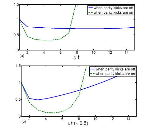
Figure 1: The variance $\langle(\Delta X)^{2}\rangle$ versus rescaled time $\ \epsilon t$ when parity kicks are on and off respectively. Figure (a) refers to a Lorentzian spectrum and figure (b) refers to an Ohmic spectrum. We find that a better squeezing can be obtained when parity kicks are applied to the system.

Discussions.— It is interesting to do a comparison between several methods, including the widely used Markovian master equation Louisell . Under the Hamiltonian (3) with a Lorentzian spectrum as shown in Ref. Liu2001 , we can obtain an exact solution

$$\begin{split}a(t)=&[u(t)e^{-\Gamma t/2}a+\sum u_{j}(t)b_{j}]e^{-i\omega t}\\ =&\{[\cos(\Theta t/2)+\frac{\Gamma}{\Theta}\sin(\Theta t/2)]+\sum u_{j}(t)b_{j}\}e^{-i\omega t}.\end{split}$$ (8)

The constant $\Theta$ is given by $\Theta=\sqrt{4\pi\eta^{2}D-\Gamma^{2}}$, where D is the density of reservoir modes and $u_{j}(t)$ are some complicated functions Liu2001 . However, the master equation, in the Markovian approximation, can be written as

$$\begin{split}\frac{\partial\rho}{\partial t}=&-i\omega[a^{{\dagger}}a,\rho]+\frac{\lambda}{2}[2a\rho a^{{\dagger}}-a^{{\dagger}}a\rho-\rho a^{{\dagger}}a]+\\ &+\lambda\overline{n}[a^{{\dagger}}\rho a+a\rho a^{{\dagger}}-a^{{\dagger}}a\rho-\rho aa^{{\dagger}}],\end{split}$$ (9)

where $\lambda=2\pi Dg(\omega)^{2}$ is a constant, which represents the decay rate of the harmonic oscillator. For simplicity, we assume the temperature of reservoir to be zero, and the initial state of system to be $|1\rangle$. We then calculate the the probability $P(t)=\langle 1|tr_{R}(\rho(t))|1\rangle$, which can be used to observe the decay of system. We can also compute $P(t)$ when the coupling strengths $\gamma_{k}$ are constants. For example, we assume that parameters of the Lorentzian spectrum in Fig 2(a) to be $\gamma_{j}=g(\omega_{j})=2.8209\times 10^{12}/\sqrt{(\omega_{j}-\omega)^{2}+10^{12}}$Hz, and the flat spectrum in Fig 2(b) to be $\gamma_{j}=5.6419\times 10^{6}$ Hz with $j=1,2,\ldots 200$. For the flat spectrum we assume the frequencies associated with the system and reservoir to be $\omega=10^{9}$Hz and $\omega_{j}=j\times 10^{7}$Hz $(j=1,2,\ldots 200)$ respectively. For the Lorentzian spectrum, however, we change the frequencies of the reservoir to be $\omega_{j}=(50+j/2)\times 10^{7}$Hz $(j=1,2,\ldots 200)$ due to the shape of the Lorentzian spectrum, which varies dramatically at the center and is negligible at two sides. By making this change we can sample the spectrum better. Then we plot Fig. 2.

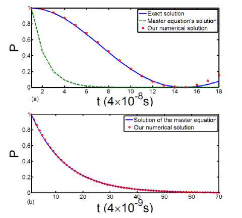
Figure 2: (a) The probability of the system being in state $|1\rangle$ with a Lorentzian spectrum. We can see that our numerical solution is close to the exact solution. On the other hand, we can see master equation is not valid for this situation. (We set the reservoir to have 200 equally distributed oscillators while getting the numerical solution of our method.) (b) The probability of the system being in state $|1\rangle$ when the coupling strengths $\gamma_{k}$ are constant. We can see that the lines of our numerical solution and master equation’s solution coincide with each other.

We can find that while the master equation leads to a good approximate solution in some cases, it fails sometimes. Thus our method is more reliable, and the accuracy can be further improved by using better numerical methods.

We also note that the parity kicks can be done by increasing the frequency of the harmonic oscillator for a short time interval. For example, this can be achieved in the ion trap by changing the electric field. (also see Refs. squ1 ; squ2 for schemes of generating squeezed states in ion trap)

Conclusions.— We have shown that for a general Hamiltonian with bononic quadratic forms, we can compute dynamics of system using exponential quadratic operators. Our method provides substantial improvement over computation involving master equations as we do not need to solve any differential equations and provides numerical solution for Hamiltonians that can be written in quadratic form of creation and annihilation operators. Thus, this new techniques compares well with the dynamics of the system under a master equation but it is in some sense more appealing as it could provide in principle analytical expressions for some cases. In particular, we analyze the effect of reservoir in a squeezing process and we propose possible scheme to improve the degree of squeezing. Our method can be applied to study the problem on the quantization of nano-mechanical systems, the further work will be presented elsewhere.

KLC acknowledges financial support by the National Research Foundation & Ministry of Education, Singapore. This work was supported in part by the National Basic Research Program of China grant No. 2007CB907900 and 2007CB807901, NSFC grant No. 60725416 and China Hi-Tech program grant No. 2006AA01Z420.

References

- (1) D. Braun, Phys. Rev. Lett. 89, 277901 (2002); J. P. Paz and A. J. Roncaglia, Phys. Rev. Lett. 100, 220401 (2008).
- (2) N. Erez, G. Gordon, M. Nest, and G. Kurizki, Nature 452, 724 (2008).
- (3) B. Misra and E. C. G. Sudarshan, J. Math. Phys. 18, 756 (1977).
- (4) D. Vitali and P. Tombesi, Phys. Rev. A 59, 4178 (1999).
- (5) L. Viola and E. Knill, Phys. Rev. Lett. 94, 060502 (2005).
- (6) K. Khodjasteh and D. A. Lidar, Phys. Rev. A 75, 062310 (2007).
- (7) M.A. de Ponte, M.C. de Oliveira, and M.H.Y. Moussa, Annals of Physics 317, 72 (2005).
- (8) A. G. Kofman and G. Kurizki, Phys. Rev. Lett. 93, 130406 (2004).
- (9) U. Herzog, Optics Communications 179, 381 (2000)
- (10) L. -A. Wu, M. S. Byrd, and D. A. Lidar, Phys. Rev. Lett. 89, 127901 (2002).
- (11) A. J. Leggett, S. Chakravarty, A. T. Dorsey, P. A. Fisher, A. Garg and W. Zwerger, Rev. Mod. Phys. 59, 1 (1987).
- (12) U. Weiss, Quantum Dissipative Systems (World Scientific, singapore, 2008).
- (13) W. H.Louisell, Quantum Statistical Properties of Radiation (John Wiley and Sons, New York, 1973).
- (14) C.W. Gardiner, Quantum Noise (Springer, Berlin, 1991).
- (15) M. O. Scully and M. S. Zubairy, Quantum optics (Cambridge University Press, Cambridge, 1997).
- (16) R. P. Feynman and F. L. Vernon, Annals of Physics 24, 181 (1963).
- (17) A. O. Caldeira and A. J. Leggett, Physica A 121, 587 (1983).
- (18) Balian and Brezin, Nuovo Cimento 64, 37 (1969).
- (19) X.B. Wang, S. X. Yu, and Y.D. Zhang, J. Phys. A: Math. Gen. 27, 6563 (1994).
- (20) X.B. Wang, C. H. Oh, and L. C. Kwek, J. Phys. A: Math. Gen. 31, 4329 (1998).
- (21) Y. X. Liu, C. P. Sun, and S. X. Yu, Phys. Rev. A 63, 033816 (2001).
- (22) J. I. Cirac, A. S. Parkins, R. Blatt, and P. Zoller, Phys. Rev. Lett. 70, 556 (1993).
- (23) H.P. Zeng and F.C. Lin, Phys. Rev. A 52, 809 (1995).