Distance Dependent Chinese Restaurant Processes

Abstract

We develop the distance dependent Chinese restaurant process, a flexible class of distributions over partitions that allows for dependencies between the elements. This class can be used to model many kinds of dependencies between data in infinite clustering models, including dependencies arising from time, space, and network connectivity. We examine the properties of the distance dependent CRP, discuss its connections to Bayesian nonparametric mixture models, and derive a Gibbs sampler for both fully observed and latent mixture settings. We study its empirical performance with three text corpora. We show that relaxing the assumption of exchangeability with distance dependent CRPs can provide a better fit to sequential data and network data. We also show that the distance dependent CRP representation of the traditional CRP mixture leads to a faster-mixing Gibbs sampling algorithm than the one based on the original formulation.

1 Introduction

Dirichlet process (DP) mixture models provide a valuable suite of flexible clustering algorithms for high dimensional data analysis. Such models have been adapted to text modeling (Teh et al., 2006; Goldwater et al., 2006), computer vision (Sudderth et al., 2005), sequential models (Dunson, 2006; Fox et al., 2007), and computational biology (Xing et al., 2007). Moreover, recent years have seen significant advances in scalable approximate posterior inference methods for this class of models (Liang et al., 2007; Daume, 2007; Blei and Jordan, 2005). DP mixtures have become a valuable tool in modern machine learning.

DP mixtures can be described via the Chinese restaurant process (CRP), a distribution over partitions that embodies the assumed prior distribution over cluster structures (Pitman, 2002). The CRP is fancifully described by a sequence of customers sitting down at the tables of a Chinese restaurant. Each customer sits at a previously occupied table with probability proportional to the number of customers already sitting there, and at a new table with probability proportional to a concentration parameter. In a CRP mixture, customers are identified with data points, and data sitting at the same table belong to the same cluster. Since the number of occupied tables is random, this provides a flexible model in which the number of clusters is determined by the data.

The customers of a CRP are exchangeable—under any permutation of their ordering, the probability of a particular configuration is the same—and this property is essential to connect the CRP mixture to the DP mixture. The reason is as follows. The Dirichlet process is a distribution over distributions, and the DP mixture assumes that the random parameters governing the observations are drawn from a distribution drawn from a Dirichlet process. The observations are conditionally independent given the random distribution, and thus they must be marginally exchangeable. If the CRP mixture did not yield an exchangeable distribution, it could not be equivalent to a DP mixture.

Exchangeability is a reasonable assumption in some clustering applications, but in many it is not. Consider data ordered in time, such as a time-stamped collection of news articles. In this setting, each article should tend to cluster with other articles that are nearby in time. Or, consider spatial data, such as pixels in an image or measurements at geographic locations. Here again, each datum should tend to cluster with other data that are nearby in space. While the traditional CRP mixture provides a flexible prior over partitions of the data, it cannot accommodate such non-exchangeability.

In this paper, we develop the distance dependent Chinese restaurant process, a new CRP in which the random seating assignment of the customers depends on the distances between them. These distances can be based on time, space, or other characteristics. Distance dependent CRPs can recover a number of existing dependent distributions (Ahmed and Xing, 2008; Zhu et al., 2005). They can also be arranged to recover the traditional CRP distribution. The distance dependent CRP expands the palette of infinite clustering models, allowing for many useful non-exchangeable distributions as priors on partitions.

The key to the distance dependent CRP is that it represents the partition with customer assignments, rather than table assignments. While the traditional CRP connects customers to tables, the distance dependent CRP connects customers to other customers. The partition of the data, i.e., the table assignment representation, arises from these customer connections. When used in a Bayesian model, the customer assignment representation allows for a straightforward Gibbs sampling algorithm for approximate posterior inference (see Section 3). This provides a new tool for flexible clustering of non-exchangeable data, such as time-series or spatial data, as well as a new algorithm for inference with traditional CRP mixtures.

Related work.

Several other non-exchangeable priors on partitions have appeared in recent research literature. Some can be formulated as distance dependent CRPs, while others represent a different class of models. The most similar to the distance dependent CRP is the probability distribution on partitions presented in Dahl (2008). Like the distance dependent CRP, this distribution may be constructed through a collection of independent priors on customer assignments to other customers, which then implies a prior on partitions. Unlike the distance dependent CRP, however, the distribution presented in Dahl (2008) requires normalization of these customer assignment probabilities. The model in Dahl (2008) may always be written as a distance dependent CRP, although the normalization requirement prevents the reverse from being true (see Section 2). We note that Dahl (2008) does not present an algorithm for sampling from the posterior, but the Gibbs sampler presented here for the distance dependent CRP can also be employed for posterior inference in that model.

There are a number of Bayesian nonparametric models that allow for dependence between (marginal) partition membership probabilities. These include the dependent Dirichlet process (MacEachern, 1999) and other similar processes (Duan et al., 2007; Griffin and Steel, 2006; Xue et al., 2007). Such models place a prior on collections of sampling distributions drawn from Dirichlet processes, with one sampling distribution drawn per possible value of covariate and sampling distributions from similar covariates more likely to be similar. Marginalizing out the sampling distributions, these models induce a prior on partitions by considering two customers to be clustered together if their sampled values are equal. (Recall, these sampled values are drawn from the sampling distributions corresponding to their respective covariates.) This prior need not be exchangeable if we do not condition on the covariate values.

Distance dependent CRPs represent an alternative strategy for modeling non-exchangeability. The difference hinges on marginal invariance, the property that a missing observation does not affect the joint distribution. In general, dependent DPs exhibit marginal invariance while distance dependent CRPs do not. For the practitioner, this property is a modeling choice, which we discuss in Section 2. Section 4 shows that distance dependent CRPs and dependent DPs represent nearly distinct classes of models, intersecting only in the original DP or CRP.

Still other prior distributions on partitions include those presented in Ahmed and Xing (2008) and Zhu et al. (2005), both of which are special cases of the distance dependent CRP. Rasmussen and Ghahramani (2002) use a gating network similar to the distance dependent CRP to partition datapoints among experts in way that is more likely to assign nearby points to the same cluster. Also included are the product partition models of Hartigan (1990), their recent extension to dependence on covariates (Muller et al., 2008), and the dependent Pitman-Yor process (Sudderth and Jordan, 2008). A review of prior probability distributions on partitions is presented in Mueller and Quintana (2008). The Indian Buffet Process, a Bayesian non-parametric prior on sparse binary matrices, has also been generalized to model non-exchangeable data by Miller et al. (2008). We further discuss these priors in relation to the distance dependent CRP in Section 2.

The rest of this paper is organized as follows. In Section 2 we develop the distance dependent CRP and discuss its properties. We show how the distance dependent CRP may be used to model discrete data, both fully-observed and as part of a mixture model. In Section 3 we show how the customer assignment representation allows for an efficient Gibbs sampling algorithm. In Section 4 we show that distance dependent CRPs and dependent DPs represent distinct classes of models. Finally, in Section 5 we describe an empirical study of three text corpora using the distance dependent CRP. We show that relaxing the assumption of exchangeability with distance dependent CRPs can provide a better fit to sequential data. We also show its alternative formulation of the traditional CRP leads to a faster-mixing Gibbs sampling algorithm than the one based on the original formulation.

2 Distance dependent CRPs

Figure 1: An illustration of the distance dependent CRP. The process operates at the level of customer assignments, where each customer chooses either another customer or no customer according to Eq. (2). Customers that chose not to connect to another are indicated with a self link The table assignments, a representation of the partition that is familiar to the CRP, are derived from the customer assignments.

Figure 2: Draws from sequential CRPs. Illustrated are draws for different decay functions, which are inset: (1) The traditional CRP; (2) The window decay function; (3) The exponential decay function; (4) The logistic decay function. The table assignments are illustrated, which are derived from the customer assignments drawn from the distance dependent CRP. The decay functions (inset) are functions of the distance between the current customer and each previous customer.

The Chinese restaurant process (CRP) is a probability distribution over partitions (Pitman, 2002). It is described by considering a Chinese restaurant with an infinite number of tables and a sequential process by which customers enter the restaurant and each sit down at a randomly chosen table. After $N$ customers have sat down, their configuration at the tables represents a random partition. Customers sitting at the same table are in the same cycle.

In the traditional CRP, the probability of a customer sitting at a table is computed from the number of other customers already sitting at that table. Let $z_{i}$ denote the table assignment of the $i$th customer, assume that the customers $z_{1:(i-1)}$ occupy $K$ tables, and let $n_{k}$ denote the number of customers sitting at table $k$. The traditional CRP draws each $z_{i}$ sequentially,

$$p(z_{i}=k\,|\,z_{1:(i-1)},\alpha)\propto\left\{\begin{array}[]{ll}n_{k}&\textrm{for}\quad k\leq K\\ \alpha&\textrm{for}\quad k=K+1,\end{array}\right.$$ (1)

where $\alpha$ is a given scaling parameter. When all $N$ customers have been seated, their table assignments provide a random partition. Though the process is described sequentially, the CRP is exchangeable. The probability of a particular partition of $N$ customers is invariant to the order in which they sat down.

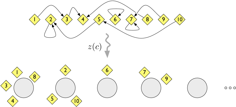
We now introduce the distance dependent CRP. In this distribution, the seating plan probability is described in terms of the probability of a customer sitting with each of the other customers. The allocation of customers to tables is a by-product of this representation. If two customers are reachable by a sequence of interim customer assignments, then they at the same table. This is illustrated in Figure 1.

Let $c_{i}$ denote the $i$th customer assignment, the index of the customer with whom the $i$th customer is sitting. Let $d_{ij}$ denote the distance measurement between customers $i$ and $j$, let $D$ denote the set of all distance measurements between customers, and let $f$ be a decay function (described in more detail below). The distance dependent CRP independently draws the customer assignments conditioned on the distance measurements,

$$p(c_{i}=j\,|\,D,\alpha)\propto\left\{\begin{array}[]{ll}f(d_{ij})&\textrm{if}\quad j\neq i\\ \alpha&\textrm{if}\quad i=j.\end{array}\right.$$ (2)

Notice the customer assignments do not depend on other customer assignments, only the distances between customers. Also notice that $j$ ranges over the entire set of customers, and so any customer may sit with any other. (If desirable, restrictions are possible through the distances $d_{ij}$. See the discussion below of sequential CRPs.)

As we mentioned above, customers are assigned to tables by considering sets of customers that are reachable from each other through the customer assignments. (Again, see Figure 1.) We denote the induced table assignments $z(\mathbf{c})$, and notice that many configurations of customer assignments $\mathbf{c}$ might lead to the same table assignment. Finally, customer assignments can produce a cycle, e.g., customer 1 sits with 2 and customer 2 sits with 1. This still determines a valid table assignment: All customers sitting in a cycle are assigned to the same table.

By being defined over customer assignments, the distance dependent CRP provides a more expressive distribution over partitions than models based on table assignments. This distribution is determined by the nature of the distance measurements and the decay function. For example, if each customer is time-stamped, then $d_{ij}$ might be the time difference between customers $i$ and $j$; the decay function can encourage customers to sit with those that are contemporaneous. If each customer is associated with a location in space, then $d_{ij}$ might be the Euclidean distance between them; the decay function can encourage customers to sit with those that are in proximity. For many sets of distance measurements, the resulting distribution over partitions is no longer exchangeable; this is an appropriate distribution to use when exchangeability is not a reasonable assumption.

Decay functions.

In general, the decay function mediates how distances between customers affect the resulting distribution over partitions. We assume that the decay function $f$ is non-increasing, takes non-negative finite values, and satisfies $f(\infty)=0$. We consider several types of decay as examples, all of which satisfy these nonrestrictive assumptions.

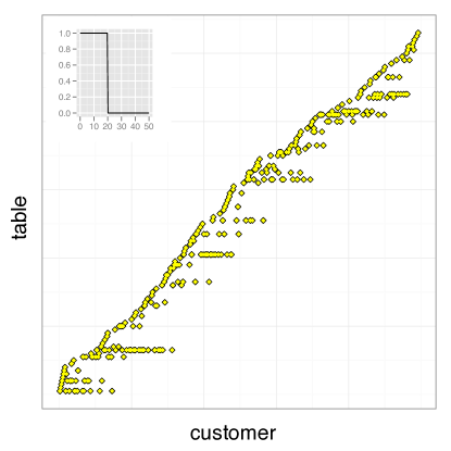
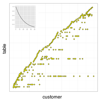
The window decay $f(d)=1[d<a]$ only considers customers that are at most distance $a$ from the current customer. The exponential decay $f(d)=e^{-d/a}$ decays the probability of linking to an earlier customer exponentially with the distance to the current customer. The logistic decay $f(d)=\exp{(-d+a)}/(1+\exp{(-d+a)})$ is a smooth version of the window decay. Each of these affects the distribution over partitions in a different way.

Sequential CRPs and the traditional CRP.

With certain types of distance measurements and decay functions, we obtain the special case of sequential CRPs. A sequential CRP is constructed by assuming that $d_{ij}=\infty$ for those $j>i$. With our previous requirement that $f(\infty)=0$, this guarantees that no customer can be assigned to a later customer, i.e., $p(c_{i}\leq i\,|\,D)=1$. The sequential CRP lets us define alternative formulations of some previous time-series models. For example, with a window decay function and $a=1$, we recover the model studied in Ahmed and Xing (2008). With a logistic decay function, we recover the model studied in Zhu et al. (2005). In our empirical study we will examine sequential models in detail.

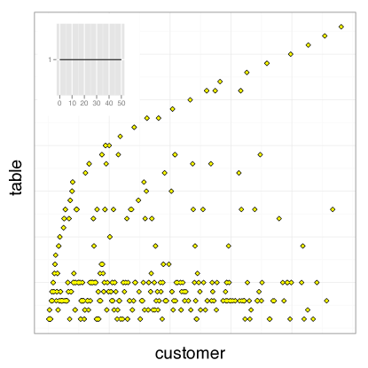
The sequential CRP can re-express the traditional CRP. Specifically, the traditional CRP is recovered when $f(d)=1$ for $d\neq\infty$ and $d_{ij}<\infty$ for $j<i$. To see this, consider the marginal distribution of a customer sitting at a particular table, given the previous customers’ assignments. The probability of being assigned to each of the other customers at that table is proportional to one. Thus, the probability of sitting at that table is proportional to the number of customers already sitting there. Moreover, the probability of not being assigned to a previous customer is proportional to the scaling parameter $\alpha$. This is precisely the traditional CRP distribution of Eq. (1). Although these models are the same, the corresponding Gibbs samplers are different (see Section 5.4).

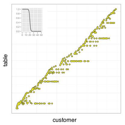
Figure 2 illustrates seating assignments (at the table level) derived from draws from sequential CRPs with each of the decay functions described above, including the original CRP. (To adapt these settings to the sequential case, the distances are $d_{ij}=i-j$ for $j<i$ and $d_{ij}=\infty$ for $j>i$.) Compared to the traditional CRP, customers tend to sit at the same table with other nearby customers. We emphasize that sequential CRPs are only one type of distance dependent CRP. Other distances, combined with the formulation of Eq. (2), lead to a variety of other non-exchangeable distributions over partitions.

Marginal invariance.

The traditional CRP is marginally invariant: Marginalizing over a particular customer gives the same probability distribution as if that customer were not included in the model at all. The distance dependent CRP does not generally have this property, allowing it to capture the way in which influence might be transmitted from one point to another. See Section 4 for a precise characterization of the class of distance dependent CRPs that are marginally invariant.

To see when this might be a relevant property, consider the goal of modeling preferences of people within a social network. The model used should reflect the fact that persons A and B are more likely to share preferences if they also share a common friend C. Any marginally invariant model, however, would insist that the distribution of the preferences of A and B is the same whether (1) they have no such common friend C, or (2) they do but his preferences are unobserved and hence marginalized out. In this setting, we might prefer a model that is not marginally invariant. Knowing that they have a common friend affects the probability that A and B share preferences, regardless of whether the friend’s preferences are observed. A similar example is modeling the spread of disease. Suddenly discovering a city between two others–even if the status of that city is unobserved–should change our assessment of the probability that the disease travels between them.

We note, however, that if observations are missing then models that are not marginally invariant require that relevant conditional distributions be computed as ratios of normalizing constants. In contrast, marginally invariant models afford a more convenient factorization, and so allow easier computation. Even when faced with data that clearly deviates from marginal invariance, the modeler may be tempted to use a marginally invariant model, choosing computational convenience over fidelity to the data.

We have described a general formulation of the distance dependent CRP. We now describe two applications to Bayesian modeling of discrete data, one in a fully observed model and the other in a mixture model. These examples illustrate how one might use the posterior distribution of the partitions, given data and an assumed generating process based on the distance dependent CRP. We will focus on models of discrete data and we will use the terminology of document collections to describe these models. Thus, our observations are assumed to be collections of words from a fixed vocabulary, organized into documents.

Language modeling.

In the language modeling application, each document is associated with a distance dependent CRP, and its tables are embellished with IID draws from a base distribution over terms or words. (The documents share the same base distribution.) The generative process of words in a document is as follows. The data are first placed at tables via customer assignments, and then assigned to the word associated with their tables. Subsets of the data exhibit a partition structure by sharing the same table.

When using a traditional CRP, this is a formulation of a simple Dirichlet-smoothed language model. Alternatives to this model, such as those using the Pitman-Yor process, have also been applied in this setting (Teh, 2006; Goldwater et al., 2006). We consider a sequential CRP, which assumes that a word is more likely to occur near itself in a document. Words are still considered contagious—seeing a word once means we’re likely to see it again—but the window of contagion is mediated by the decay function.

More formally, given a decay function $f$, sequential distances $D$, scaling parameter $\alpha$, and base distribution $G_{0}$ over discrete words, $N$ words are drawn as follows,

1. For each word $i\in\{1,\ldots,N\}$ draw assignment $c_{i}\sim\textrm{dist-CRP}(\alpha,f,D)$.

2. For each table, $k\in\{1,\ldots\}$, draw a word $w^{*}\sim G_{0}$.

3. For each word $i\in\{1,\ldots,N\}$, assign the word $w_{i}=w^{*}_{z(\mathbf{c})_{i}}$.

The notation $z(\mathbf{c})_{i}$ is the table assignment of the $i$th customer in the table assignments induced by the complete collection of customer assignments.

For each document, we observe a sequence of words $w_{1:N}$ from which we can infer their seating assignments in the distance dependent CRP. The partition structure of observations—that is, which words are the same as other words—indicates either that they share the same table in the seating arrangement, or that two tables share the same term drawn from $G_{0}$. We have not described the process sequentially, as one would with a traditional CRP, in order to emphasize the three stage process of the distance dependent CRP—first the customer assignments and table parameters are drawn, and then the observations are assigned to their corresponding parameter. However, the sequential distances $D$ guarantee that we can draw each word successively. This, in turn, means that we can easily construct a predictive distribution of future words given previous words. (See Section 3 below.)

Mixture modeling

The second model we study is akin to the CRP mixture or (equivalently) the DP mixture, but differs in that the mixture component for a data point depends on the mixture component for nearby data. Again, each table is endowed with a draw from a base distribution $G_{0}$, but here that draw is a distribution over mixture component parameters. In the document setting, observations are documents (as opposed to individual words), and $G_{0}$ is typically a Dirichlet distribution over distributions of words (Teh et al., 2006). The data are drawn as follows:

1. For each document $i\in[1,N]$ draw assignment $c_{i}\sim\textrm{dist-CRP}(\alpha,f,D)$.

2. For each table, $k\in\{1,\ldots\}$, draw a parameter $\theta_{k}^{*}\sim G_{0}$.

3. For each document $i\in[1,N]$, draw $w_{i}\sim F(\theta_{z(\mathbf{c})_{i}})$.

In Section 5, we will study the sequential CRP in this setting, choosing its structure so that contemporaneous documents are more likely to be clustered together. The distances $d_{ij}$ can be the differences between indices in the ordering of the data, or lags between external measurements of distance like date or time. (Spatial distances or distances based on other covariates can be used to define more general mixtures, but we leave these settings for future work.) Again, we have not defined the generative process sequentially but, as long as $D$ respects the assumptions of a sequential CRP, an equivalent sequential model is straightforward to define.

Relationship to dependent Dirichlet processes.

More generally, the distance dependent CRP mixture provides an alternative to the dependent Dirichlet process (DDP) mixture as an infinite clustering model that models dependencies between the latent component assignments of the data (MacEachern, 1999). The DDP has been extended to sequential, spatial, and other kinds of dependence (Griffin and Steel, 2006; Duan et al., 2007; Xue et al., 2007). In all these settings, statisticians have appealed to truncations of the stick-breaking representation for approximate posterior inference, citing the dependency between data as precluding the more efficient techniques that integrate out the component parameters and proportions. In contrast, distance dependent CRP mixtures are amenable to Gibbs sampling algorithms that integrate out these variables (see Section 3).

An alternative to the DDP formalism is the Bayesian density regression (BDR) model of Dunson et al. (2007). In BDR, each data point is associated with a random measure and is drawn from a mixture of per-data random measures where the mixture proportions are related to the distance between data points. Unlike the DDP, this model affords a Gibbs sampler where the random measures can be integrated out.

However, it is still different in spirit from the distance dependent CRP. Data are drawn from distributions that are similar to distributions of nearby data, and the particular values of nearby data impose softer constraints than those in the distance dependent CRP. As an extreme case, consider a random partition of the nodes of a network, where distances are defined in terms of the number of hops between nodes. Further, suppose that there are several disconnected components in this network, that is, pairs of nodes that are not reachable from each other. In the DDP model, these nodes are very likely not to be partitioned in the same group. In the ddCRP model, however, it is impossible for them to be grouped together.

We emphasize that DDP mixtures (and BDR) and distance dependent CRP mixtures are different classes of models. DDP mixtures are Bayesian nonparametric models, interpretable as data drawn from a random measure, while the distance dependent CRP mixtures generally are not. DDP mixtures exhibit marginal invariance, while distance dependent CRPs generally do not (see Section 4). In their ability to capture dependence, these two classes of models capture similar assumptions, but the appropriate choice of model depends on the modeling task at hand.

3 Posterior inference and prediction

The central computational problem for distance dependent CRP modeling is posterior inference, determining the conditional distribution of the hidden variables given the observations. This posterior is used for exploratory analysis of the data and how it clusters, and is needed to compute the predictive distribution of a new data point given a set of observations.

Regardless of the likelihood model, the posterior will be intractable to compute because the distance dependent CRP places a prior over a combinatorial number of possible customer configurations. In this section we provide a general strategy for approximating the posterior using Monte Carlo Markov chain (MCMC) sampling. This strategy can be used in either fully-observed or mixture settings, and can be used with arbitrary distance functions. (For example, in Section 5 we illustrate this algorithm with both sequential distance functions and graph-based distance functions and in both fully-observed and mixture settings.)

In MCMC, we aim to construct a Markov chain whose stationary distribution is the posterior of interest. For distance dependent CRP models, the state of the chain is defined by $c_{i}$, the customer assignments for each data point. We will also consider $z(\mathbf{c})$, which are the table assignments that follow from the customer assignments (see Figure 1). Let $\eta=\{D,\alpha,f,G_{0}\}$ denote the set of model hyperparameters. It contains the distances $D$, the scaling factor $\alpha$, the decay function $f$, and the base measure $G_{0}$. Let $x$ denote the observations.

In Gibbs sampling, we iteratively draw from the conditional distribution of each latent variable given the other latent variables and observations. (This defines an appropriate Markov chain, see Neal (1993).) In distance dependent CRP models, the Gibbs sampler iteratively draws from

$$p(c_{i}^{\textrm{(new)}}\,|\,\mathbf{c}_{-i},\mathbf{x},\eta)\propto p(c_{i}^{\textrm{(new)}}\,|\,D,\alpha)p(\mathbf{x}\,|\,z(\mathbf{c}_{-i}\cup c_{i}^{\textrm{(new)}}),G_{0}).$$ (3)

The first term is the distance dependent CRP prior from Eq. (2).

The second term is the likelihood of the observations under the partition given by $z(\mathbf{c}_{-i}\cup c_{i}^{(new)})$. This can be thought of as removing the current link from the $i$th customer and then considering how each alternative new link affects the likelihood of the observations. Before examining this likelihood, we describe how removing and then replacing a customer link affects the underlying partition (i.e., table assignments).

Figure 3: An example of a single step of the Gibbs sampler. Here we illustrate a scenario that highlights all the ways that the sampler can move: A table can be split when we remove the customer link before conditioning; and two tables can join when we resample that link.

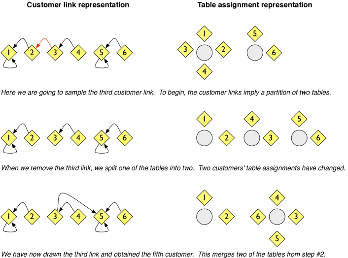
To begin, consider the effect of removing a customer link. What is the difference between the partition $z(\mathbf{c})$ and $z(\mathbf{c}_{-i})$? There are two cases.

The first case is that a table splits. This happens when $c_{i}$ is the only connection between the $i$th data point and a particular table. Upon removing $c_{i}$, the customers at its table are split in two: those customers pointing (directly or indirectly) to $i$ are at one table; the other customers previously seated with $i$ are at a different table. (See the change from the first to second rows of Figure 3.)

The second case is that there is no change. If the $i$th link is not the only connection between customer $i$ and his table or if $c_{i}$ was a self-link ($c_{i}=i$) then the tables remain the same. In this case, $z(\mathbf{c}_{-i})=z(\mathbf{c})$.

Now consider the effect of replacing the customer link. What is the difference between the partition $z(\mathbf{c}_{-i})$ and $z(\mathbf{c}_{-i}\cup c_{i}^{\textrm{(new)}})$? Again there are two cases. The first case is that $c_{i}^{\textrm{(new)}}$ joins two tables in $z(\mathbf{c}_{-i})$. Upon adding $c_{i}^{\textrm{(new)}}$, the customers at its table become linked to another set of customers. (See the change from the second to third rows of Figure 3.)

The second case, as above, is that there is no change. This occurs if $c_{i}^{\textrm{(new)}}$ points to a customer that is already at its table under $z(\mathbf{c}_{-i})$ or if $c_{i}^{\textrm{(new)}}$ is a self-link.

With the changed partition in hand, we now compute the likelihood term. We first compute the likelihood term for partition $z(\mathbf{c})$. The likelihood factors into a product of terms, each of which is the probability of the set of observations at each table. Let $|z(\mathbf{c})|$ be the number of tables and $z^{k}(\mathbf{c})$ be the set of indices that are assigned to table $k$. The likelihood term is

$$p(\mathbf{x}\,|\,z(\mathbf{c}),G_{0})=\prod_{k=1}^{|z(\mathbf{c})|}p(\mathbf{x}_{z^{k}(\mathbf{c})}\,|\,G_{0}).$$ (4)

Because of this factorization, the Gibbs sampler need only compute terms that correspond to changes in the partition. Consider the partition $z(\mathbf{c}_{-i})$, which may have split a table, and the new partition $z(\mathbf{c}_{-i}\cup c^{\textrm{(new)}})$. There are three cases to consider. First, $c_{i}$ might link to itself—there will be no change to the likelihood function because a self-link cannot join two tables. Second, $c_{i}$ might link to another table but cause no change in the partition. Finally, $c_{i}$ might link to another table and join two tables $k$ and $\ell$. The Gibbs sampler for the distance dependent CRP is thus

$$p(c_{i}^{\textrm{(new)}}\,|\,\mathbf{c}_{-i},\mathbf{x},\eta)\propto\left\{\begin{array}[]{ll}\alpha&\textrm{if }c_{i}^{\textrm{(new)}}\textrm{ is equal to }i.\\ f(d_{ij})&\textrm{if }c_{i}^{\textrm{(new)}}=j\textrm{ does not join two tables.}\\ f(d_{ij})\large\frac{p(\mathbf{x}_{z^{k}(\mathbf{c}_{-i})\cup z^{\ell}(\mathbf{c}_{-i})}\,|\,G_{0})}{p(\mathbf{x}_{z^{k}(\mathbf{c}_{-i})}\,|\,G_{0})p(\mathbf{x}_{z^{\ell}(\mathbf{c}_{-i})}\,|\,G_{0})}&\textrm{if }c_{i}^{\textrm{(new)}}=j\textrm{ joins tables }k\textrm{ and }\ell.\end{array}\right.$$ (5)

The specific form of the terms in Eq. (4) depend on the model. We first consider the fully observed case (i.e., “language modeling”). Recall that the partition corresponds to words of the same type, but that more than one table can contain identical types. (For example, four tables could contain observations of the word “peanut.” But, observations of the word “walnut” cannot sit at any of the peanut tables.) Thus, the likelihood of the data is simply the probability under $G_{0}$ of a representative from each table, e.g., the first customer, times a product of indicators to ensure that all observations are equal,

$$p(\mathbf{x}_{z^{k}(\mathbf{c})}\,|\,G_{0})=p(x_{z^{k}(\mathbf{c})_{1}}\,|\,G_{0})\textstyle\prod_{i\in z^{k}(\mathbf{c})}1(x_{i}=x_{z^{k}(\mathbf{c})_{1}}),$$ (6)

where $z^{k}(\mathbf{c})_{1}$ is the index of the first customer assigned to table $k$.

In the mixture model, we compute the marginal probability that the set of observations from each table are drawn independently from the same parameter, which itself is drawn from $G_{0}$. Each term is

$$p(\mathbf{x}_{z^{k}(\mathbf{c})}\,|\,G_{0})=\int\textstyle\left(\prod_{i\in z^{k}(\mathbf{c})}p(x_{i}\,|\,\theta)\right)p(\theta\,|\,G_{0})d\theta.$$ (7)

Because this term marginalizes out the mixture component $\theta$, the result is a collapsed sampler for the mixture model. When $G_{0}$ and $p(x\,|\,\theta)$ form a conjugate pair, the integral is straightforward to compute. In nonconjugate settings, an additional layer of sampling is needed.

Prediction.

In prediction, our goal is to compute the conditional probability distribution of a new data point $x_{\textrm{new}}$ given the data set $\mathbf{x}$. This computation relies on the posterior. Recall that $D$ is the set of distances between all the data points. The predictive distribution is

$$p(x_{\textrm{new}}|\mathbf{x},D,G_{0},\alpha)=\sum_{c_{\textrm{new}}}p(c_{\textrm{new}}\,|\,D,\alpha)\textstyle\sum_{\mathbf{c}}p(x_{\textrm{new}}|c_{\textrm{new}},\mathbf{c},\mathbf{x},G_{0})p(\mathbf{c}|\mathbf{x},D,\alpha,G_{0}).$$ (8)

The outer summation is over the customer assignment of the new data point; its prior probability only depends on the distance matrix $D$. The inner summation is over the posterior customer assignments of the data set; it determines the probability of the new data point conditioned on the previous data and its partition. In this calculation, the difference between sequential distances and arbitrary distances is important.

Consider sequential distances and suppose that $x_{\textrm{new}}$ is a future data point. In this case, the distribution of the data set customer assignments $\mathbf{c}$ does not depend on the new data point’s location in time. The reason is that data points can only connect to data points in the past. Thus, the posterior $p(\mathbf{c}\,|\,\mathbf{x},D,\alpha,G_{0})$ is unchanged by the addition of the new data, and we can use previously computed Gibbs samples to approximate it.

In other situations—nonsequential distances or sequential distances where the new data occurs somewhere in the middle of the sequence—the discovery of the new data point changes the posterior $p(\mathbf{c}\,|\,\mathbf{x},D,\alpha,G_{0})$. The reason is that the knowledge of where the new data is relative to the others (i.e., the information in $D$) changes the prior over customer assignments and thus changes the posterior as well. This new information requires rerunning the Gibbs sampler to account for the new data point. Finally, note that the special case where we know the new data’s location in advance (without knowing its value) does not require rerunning the Gibbs sampler.

4 Marginal invariance

In Section 2 we discussed the property of marginal invariance, where removing a customer leaves the partition distribution over the remaining customers unchanged. When a model has this property, unobserved data may simply be ignored. We mentioned that the traditional CRP is marginally invariant, while the distance dependent CRP does not necessarily have this property.

In fact, the traditional CRP is the only distance dependent CRP that is marginally invariant. The details of this characterization are given in the appendix. This characterization of marginally invariant CRPs contrasts the distance dependent CRP with the alternative priors over partitions induced by random measures, such as the Dirichlet process.

In addition to the Dirichlet process, random-measure models include the dependent Dirichlet process (MacEachern, 1999) and the order-based dependent Dirichlet process (Griffin and Steel, 2006). These models suppose that data from a given covariate were drawn independently from a fixed latent sampling probability measure. These models then suppose that these sampling measures were drawn from some parent probability measure. Dependence between the randomly drawn sampling measures is achieved through this parent probability measure.

We formally define a random-measure model as follows. Let $\mathbb{X}$ and $\mathbb{Y}$ be the sets in which covariates and observations take their values, let $x_{1:N}\subset\mathbb{X}$, $y_{1:N}\subset\mathbb{Y}$ be the set of observed covariates and their corresponding sampled values, and let $M(\mathbb{Y})$ be the space of probability measures on $\mathbb{Y}$. A random-measure model is any probability distribution on the samples $y_{1:N}$ induced by a probability measure $G$ on the space $M(\mathbb{Y})^{\mathbb{X}}$. This random-measure model may be written

$$y_{n}\mid x_{n}\sim\mathbb{P}_{x_{n}},\qquad\left(\mathbb{P}_{x}\right)_{x\in\mathbb{X}}\sim G,$$ (9)

where the $y_{n}$ are conditionally independent of each other given $(\mathbb{P}_{x})_{x\in\mathbb{X}}$. Such models implicitly induce a distribution on partitions of the data by taking all points $n$ whose sampled values $y_{n}$ are equal to be in the same cluster.

In such random-measure models, the (prior) distribution on $y_{-n}$ does not depend on $x_{n}$, and so such models are marginally invariant, regardless of the points $x_{1:n}$ and the distances between them. From this observation, and the lack of marginal invariance of the distance dependent CRP, it follows that the distributions on partitions induced by random-measure models are different from the distance dependent CRP. The only distribution that is both a distance dependent CRP, and is also induced by a random-measure model, is the traditional CRP.

Thus, distance dependent CRPs are generally not marginally invariant, and so are appropriate for modeling situations that naturally depart from marginal invariance. This distinguishes priors obtained with distance dependent CRPs from those obtained from random-measure models, which are appropriate when marginal invariance is a reasonable assumption.

5 Empirical study

We studied the distance dependent CRP in the language modeling and mixture settings on four text data sets. We explored both time dependence, where the sequential ordering of the data is respected via the decay function and distance measurements, and network dependence, where the data are connected in a graph. We show below that the distance dependent CRP gives better fits to text data in both the fully-observed and mixture modeling settings.

Further, we compared the traditional Gibbs sampler for DP mixtures to the Gibbs sampler for the distance dependent CRP formulation of DP mixtures. We found that the sampler based on customer assignments mixes faster than the traditional sampler.

5.1 Language modeling

Figure 4: Bayes factors of the distance dependent CRP versus the traditional CRP on documents from Science and the New York Times. The black line at $0$ denotes an equal fit between the traditional CRP and distance dependent CRP, while positive values denote a better fit for the distance dependent CRP. Also illustrated are standard errors across documents.

We evaluated the fully-observed distance dependent CRP models on two data sets: a collection of 100 OCR’ed documents from the journal Science and a collection of 100 world news articles from the New York Times. We modeled each document independently. We assess sampler convergence visually, examining the autocorrelation plots of the log likelihood of the state of the chain (Robert and Casella, 2004).

We compare models by estimating the Bayes factor, the ratio of the probability under the distance dependent CRP to the probability under the traditional CRP (Kass and Raftery, 1995). For a decay function $f$, this Bayes factor is

$$BF_{f,\alpha}=p(w_{1:N}\,|\,\textrm{dist-CRP}_{f,\alpha})/p(w_{1:N}\,|\,\textrm{CRP}_{\alpha}).$$ (10)

A value greater than one indicates an improvement of the distance dependent CRP over the traditional CRP. Following Geyer and Thompson (1992), we estimate this ratio with a Monte Carlo estimate from posterior samples.

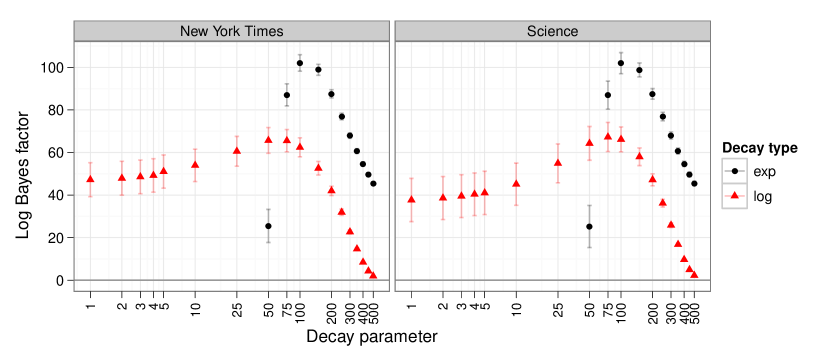
Figure 4 illustrates the average log Bayes factors across documents for various settings of the exponential and logistic decay functions. The logistic decay function always provides a better model than the traditional CRP; the exponential decay function provides a better model at certain settings of its parameter. (These curves are for the hierarchical setting with the base distribution over terms $G_{0}$ unobserved; the shapes of the curves are similar in the non-hierarchical settings.)

5.2 Mixture modeling

Figure 5: Predictive held-out log likelihood for the last year of NIPS and last three days of the New York Times corpus. Error bars denote standard errors across MCMC samples. On the NIPS data, the distance dependent CRP outperforms the traditional CRP for the logistic decay with a decay parameter of $2$ years. On the New York Times data, the distance dependent CRP outperforms the traditional CRP in almost all settings tested.

We examined the distance dependent CRP mixture on two text corpora. We analyzed one month of the New York Times (NYT) time-stamped by day, containing 2,777 articles, 3,842 unique terms and 530K observed words. We also analyzed 12 years of NIPS papers time-stamped by year, containing 1,740 papers, 5,146 unique terms, and 1.6M observed words. Distances $D$ were differences between time-stamps.

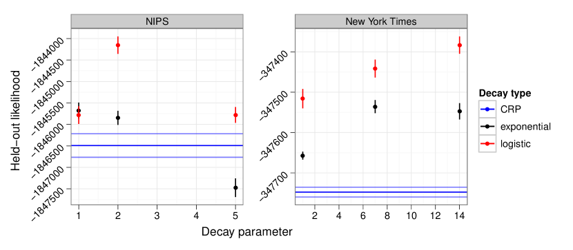
In both corpora we removed the last 250 articles as held out data. In the NYT data, this amounts to three days of news; in the NIPS data, this amounts to papers from the 11th and 12th year. (We retain the time stamps of the held-out articles because the predictive likelihood of an article’s contents depends on its time stamp, as well as the time stamps of earlier articles.) We evaluate the models by estimating the predictive likelihood of the held out data. The results are in Figure 5. On the NYT corpus, the distance dependent CRPs definitively outperform the traditional CRP. A logistic decay with a window of 14 days performs best. On the NIPS corpus, the logistic decay function with a decay parameter of 2 years outperforms the traditional CRP. In general, these results show that non-exchangeable models given by the distance dependent CRP mixture provide a better fit than the exchangeable CRP mixture.

5.3 Modeling networked data

The previous two examples have considered data analysis settings with a sequential distance function. However, the distance dependent CRP is a more general modeling tool. Here, we demonstrate its flexibility by analyzing a set of networked documents with a distance dependent CRP mixture model. Networked data induces an entirely different distance function, where any data point may link to an arbitrary set of other data. We emphasize that we can use the same Gibbs sampling algorithms for both the sequential and networked settings.

Specifically, we analyzed the CORA data set, a collection of Computer Science abstracts that are connected if one paper cites the other (McCallum et al., 2000). One natural distance function is the number of connections between data (and $\infty$ if two data points are not reachable from each other). We use the window decay function with parameter $1$, enforcing that a customer can only link to itself or to another customer that refers to an immediately connected document. We treat the graph as undirected.

Figure 6: The MAP clustering of a subset of CORA. Each node is an abstract in the collection and each link represents a citation. Colors are repeated across connected components – no two data points from disconnected components in the graph can be assigned to the same cluster. Within each connected component, colors are not repeated, and nodes with the same color are assigned to the same cluster.

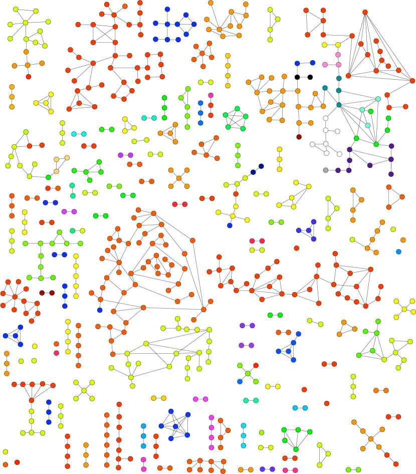
Figure 6 shows a subset of the MAP estimate of the clustering under these assumptions. Note that the clusters form connected groups of documents, though several clusters are possible within a large connected group. Traditional CRP clustering does not lean towards such solutions. Overall, the distance dependent CRP provides a better model. The log Bayes factor is 13,062, strongly in favor of the distance dependent CRP, although we emphasize that much of this improvement may occur simply because the distance dependent CRP avoids clustering abstracts from unconnected components of the network. Further analysis is needed to understand the abilities of the distance dependent CRP beyond those of simpler network-aware clustering schemes.

We emphasize that this analysis is meant to be a proof of concept to demonstrate the flexibility of distance dependent CRP mixtures. Many modeling choices can be explored, including longer windows in the decay function and treating the graph as a directed graph. A similar modeling set-up could be used to analyze spatial data, where distances are natural to compute, or images (e.g., for image segmentation), where distances might be the Manhattan distance between pixels.

5.4 Comparison to the traditional Gibbs sampler

The distance dependent CRP can express a number of flexible models. However, as we describe in Section 2, it can also re-express the traditional CRP. In the mixture model setting, the Gibbs sampler of Section 3 thus provides an alternative algorithm for approximate posterior inference in DP mixtures. We compare this Gibbs sampler to the widely used collapsed Gibbs sampler for DP mixtures, i.e., Algorithm 3 from Neal (2000), which is applicable when the base measure $G_{0}$ is conjugate to the data generating distribution.

The Gibbs sampler for the distance dependent CRP iteratively samples the customer assignment of each data point, while the collapsed Gibbs sampler iteratively samples the cluster assignment of each data point. The practical difference between the two algorithms is that the distance dependent CRP based sampler can change several customers’ cluster assignments via a single customer assignment. This allows for larger moves in the state space of the posterior and, we will see below, faster mixing of the sampler.

Moreover, the computational complexity of the two samplers is the same. Both require computing the change in likelihood of adding or removing either a set of points (in the distance dependent CRP case) or a single point (in the traditional CRP case) to each cluster. Whether adding or removing one or a set of points, this amounts to computing a ratio of normalizing constants for each cluster, and this is where the bulk of the computation of each sampler lies.

Figure 7: Each panel illustrates 100 Gibbs runs using Algorithm 3 of  (Neal, 2000) (CRP, in blue) and the sampler from Section 3 with the identity decay function (distance dependent CRP, in red). Both samplers have the same limiting distribution because the distance dependent CRP with identity decay is the traditional CRP. We plot the log probability of the CRP representation (i.e., the divergence) as a function of its iteration. The left panel shows the Science corpus, and the right panel shows the New York Times corpus. Higher values indicate that the chain has found a better local mode of the posterior. In these examples, the distance dependent CRP Gibbs sampler mixes faster.

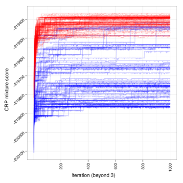
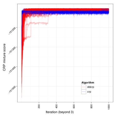
To compare the samplers, we analyzed documents from the Science and New York Times collections under a CRP mixture with scaling parameter equal to one and uniform Dirichlet base measure. Figure 7 illustrates the log probability of the state of the traditional CRP Gibbs sampler as a function of Gibbs sampler iteration. The log probability of the state is proportional to the posterior; a higher value indicates a state with higher posterior likelihood. These numbers are comparable because the models, and thus the normalizing constant, are the same for both the traditional representation and customer based CRP. Iterations 3–1000 are plotted, where each sampler is started at the same (random) state. The traditional Gibbs sampler is much more prone to stagnation at local optima, particularly for the Science corpus.

6 Discussion

We have developed the distance dependent Chinese restaurant process, a distribution over partitions that accommodates a flexible and non-exchangeable seating assignment distribution. The distance dependent CRP hinges on the customer assignment representation. We derived a general-purpose Gibbs sampler based on this representation, and examined sequential models of text.

The distance dependent CRP opens the door to a number of further developments in infinite clustering models. We plan to explore spatial dependence in models of natural images, and multi-level models akin to the hierarchical Dirichlet process (Teh et al., 2006). Moreover, the simplicity and fixed dimensionality of the corresponding Gibbs sampler suggests that a variational method is worth exploring as an alternative deterministic form of approximate inference.

Appendix A A formal characterization of marginal invariance

In this section, we formally characterize the class of distance dependent CRPs that are marginally invariant. This family is a very small subset of the entire set of distance dependent CRPs, containing only the traditional CRP and variants constructed from independent copies of it. This characterization is used in Section 4 to contrast the distance dependent CRP with random-measure models.

Throughout this section, we assume that the decay function satisfies a relaxed version of the triangle inequality, which uses the notation $\bar{d}_{ij}=\min(d_{ij},d_{ji})$. We assume: if $\bar{d}_{ij}=0$ and $\bar{d}_{jk}=0$ then $\bar{d}_{ik}=0$; and if $\bar{d}_{ij}<\infty$ and $\bar{d}_{jk}<\infty$ then $\bar{d}_{ik}<\infty$.

A.1 Sequential Distances

We first consider sequential distances. We begin with the following proposition, which shows that a very restricted class of distance dependent CRPs may also be constructed by collections of independent CRPs.

Proposition 1.

Fix a set of sequential distances between each of $n$ customers, a real number $a>0$, and a set $A\in\{\emptyset,\{0\},\mathbb{R}\}$. Then there is a (non-random) partition $B_{1},\ldots,B_{K}$ of $\{1,\ldots,n\}$ for which two distinct customers $i$ and $j$ are in the same set $B_{k}$ iff $\bar{d}_{ij}\in A$. For each $k=1,\ldots,K$, let there be an independent CRP with concentration parameter $\alpha/a$, and let customers within $B_{k}$ be clustered among themselves according to this CRP.

Then, the probability distribution on clusters induced by this construction is identical to the distance dependent CRP with decay function $f(d)=a1[d\in A]$. Furthermore, this probability distribution is marginally invariant.

Proof.

We begin by constructing a partition $B_{1},\ldots,B_{K}$ with the stated property. Let $J(i)=\min\{j:\text{$j=i$ or $\bar{d}_{ij}\in A$}\}$, and let $\mathcal{J}=\{J(i):i=1,\ldots,n\}$ be the set of unique values taken by $J$. Each customer $i$ will be placed in the set containing customer $J(i)$. Assign to each value $j\in\mathcal{J}$ a unique integer $k(j)$ between $1$ and $|\mathcal{J}|$. For each $j\in\mathcal{J}$, let $B_{k(j)}=\{i:J(i)=j\}=\{i:\text{$i=j$ or $\bar{d}_{ij}\in A$}\}$. Each customer $i$ is in exactly one set, $B_{k(J(i))}$, and so $B_{1},\ldots,B_{|\mathcal{J}|}$ is a partition of $\{1,\ldots,n\}$.

To show that $i\neq i^{\prime}$ are both in $B_{k}$ iff $\bar{d}_{ii^{\prime}}\in A$, we consider two possibilties. If $A=\emptyset$, then $J(i)=i$ and each $B_{k}$ contains only a single point. If $A=\{0\}$ or $A=\mathbb{R}$, then it follows from the relaxed triangle inequality assumed at the beginning of Appendix A.

With this partition $B_{1},\ldots,B_{K}$, the probability of linkage under the distance dependent CRP with decay function $f(d)=a1[d\in A]$ may be written

$$p(c_{i}=j)\propto\begin{cases}\alpha&\text{if $i=j$,}\\ a&\text{if $j<i$ and $j\in B_{k(i)}$,}\\ 0&\text{if $j>i$ or $j\notin B_{k(i)}$.}\end{cases}$$

By noting that linkages between customers from different sets $B_{k}$ occur with probability $0$, we see that this is the same probability distribution produced by taking $K$ independent distance dependent CRPs, where the $k$th distance dependent CRP governs linkages between customers in $B_{k}$ using

$$p(c_{i}=j)\propto\begin{cases}\alpha&\text{if $i=j$,}\\ a&\text{if $j<i$,}\\ 0&\text{if $j>i$,}\end{cases}$$

for $i,j\in B_{k}$.

Finally, dividing the unnormalized probabilities by $a$, we rewrite the linkage probabilities for the $k$th distance dependent CRP as

$$p(c_{i}=j)\propto\begin{cases}\alpha/a&\text{if $i=j$,}\\ 1&\text{if $j<i$,}\\ 0&\text{if $j>i$,}\end{cases}$$

for $i,j\in B_{k}$. This is identical to the distribution of the traditional CRP with concentration parameter $\alpha/a$.

This shows that the distance dependent CRP with decay function $f(d)=a1[d\in A]$ induces the same probability distribution on clusters as the one produced by a collection of $K$ independent traditional CRPs, each with concentration parameter $\alpha/a$, where the $k$th traditional CRP governs the clusters of customers within $B_{k}$.

The marginal invariance of this distribution follows from the marginal invariance of each traditional CRP, and their independence from one another. ∎

The probability distribution described in this proposition separates customers into groups $B_{1},\ldots,B_{K}$ based on whether inter-customer distances fall within the set $A$, and then governs clustering within each group independently using a traditional CRP. Clustering across groups does not occur.

We consider what this means for specific choices of $A$. If $A=\{0\}$, then each group contains those customers whose distance from one another is $0$. This group is well-defined because of the assumption that $d_{ij}=0$ and $d_{jk}=0$ implies $d_{ik}=0$. If $A=\mathbb{R}$, then each group contains those customers whose distance from one another is finite. Similarly to the $A=\{0\}$ case, this group is well-defined because of the assumption that $d_{ij}<\infty$ and $d_{jk}<\infty$ implies $d_{ik}<\infty$. If $A=\emptyset$, then each group contains only a single customer. In this case, each customer will be in his own cluster.

Since the resulting construction is marginally invariant, Proposition 1 provides a sufficient condition for marginal invariance. The following proposition shows that this condition is necessary as well.

Proposition 2.

If the distance dependent CRP for a given decay function $f$ is marginally invariant over all sets of sequential distances then $f$ is of the form $f(d)=a1[d\in A]$ for some $a>0$ and $A$ equal to either $\emptyset$, $\{0\}$, or $\mathbb{R}$.

Proof.

Consider a setting with $3$ customers, in which customer $2$ may either be absent, or present with his seating assignment marginalized out. Fix a non-increasing decay function $f$ with $f(\infty)=0$ and suppose that the distances are sequential, so $d_{13}=d_{23}=d_{12}=\infty$. Suppose that the distance dependent CRP resulting from this $f$ and any collection of sequential distances is marginally invariant. Then the probability that customers $1$ and $3$ share a table must be the same whether customer $2$ is absent or present.

If customer $2$ is absent,

$$\mathbb{P}\left\{\text{$1$ and $3$ sit at same table}\mid\text{$2$ absent}\right\}=\frac{f(d_{31})}{f(d_{31})+\alpha}.$$ (11)

If customer $2$ is present, customers $1$ and $3$ may sit at the same table in two different ways: $3$ sits with $1$ directly ($c_{3}=1$); or $3$ sits with $2$, and $2$ sits with $1$ ($c_{3}=2$ and $c_{2}=1$). Thus,

$$\mathbb{P}\left\{\text{$1$ and $3$ sit at same table}\mid\text{$2$ present}\right\}\\ =\frac{f(d_{31})}{f(d_{31})+f(d_{32})+\alpha}+\left(\frac{f(d_{32})}{f(d_{31})+f(d_{32})+\alpha}\right)\left(\frac{f(d_{21})}{f(d_{21})+\alpha}\right).$$ (12)

For the distance dependent CRP to be marginally invariant, Eq. (11) and Eq. (12) must be identical. Writing Eq. (11) on the left side and Eq. (12) on the right, we have

$$\frac{f(d_{31})}{f(d_{31})+\alpha}=\frac{f(d_{31})}{f(d_{31})+f(d_{32})+\alpha}+\left(\frac{f(d_{32})}{f(d_{31})+f(d_{32})+\alpha}\right)\left(\frac{f(d_{21})}{f(d_{21})+\alpha}\right).$$ (13)

We now consider two different possibilities for the distances $d_{32}$ and $d_{21}$, always keeping $d_{31}=d_{21}+d_{32}$.

First, suppose $d_{21}=0$ and $d_{32}=d_{31}=d$ for some $d\geq 0$. By multiplying Eq. (13) through by $\left(2f(d)+\alpha\right)\left(f(0)+\alpha\right)\left(f(d)+\alpha\right)$ and rearranging terms, we obtain

$$0=\alpha f(d)\left(f(0)-f(d)\right).$$

Thus, either $f(d)=0$ or $f(d)=f(0)$. Since this is true for each $d\geq 0$ and $f$ is nonincreasing, $f=a1[d\in A]$ with $a\geq 0$ and either $A=\emptyset$, $A=\mathbb{R}$, $A=[0,b]$, or $A=[0,b)$ with $b\in[0,\infty)$. Because $A=\emptyset$ is among the choices, we may assume $a>0$ without loss of generality. We now show that if $A=[0,b]$ or $A=[0,b)$, then we must have $b=0$ and $A$ is of the form claimed by the proposition.

Suppose for contradiction that $A=[0,b]$ or $A=[0,b)$ with $b>0$. Consider distances given by $d_{32}=d_{21}=d=b-\epsilon$ with $\epsilon\in(0,b/2)$. By multiplying Eq. (12) through by

$$\left(f(2d)+f(d)+\alpha\right)\left(f(d)+\alpha\right)\left(f(2d)+\alpha\right)$$

and rearranging terms, we obtain

$$0=\alpha f(d)\left(f(d)-f(2d)\right).$$

Since $f(d)=a>0$, we must have $f(2d)=f(d)>0$. But, $2d=2(b-\epsilon)>b$ implies together with $f(2d)=a1[2d\in A]$ that $f(2d)=0$, which is a contradiction. ∎

These two propositions are combined in the following corollary, which states that the class of decay functions considered in Propositions 1 and 2 is both necessary and sufficient for marginal invariance.

Corollary 1.

Fix a particular decay function $f$. The distance dependent CRP resulting from this decay function is marginally invariant over all sequential distances if and only if $f$ is of the form $f(d)=a1[d\in A]$ for some $a>0$ and some $A\in\{\emptyset,\{0\},\mathbb{R}\}$.

Proof.

Sufficiency for marginal invariance is shown by Proposition 1. Necessity is shown by Proposition 2. ∎

Although Corollary 1 allows any choice of $a>0$ in the decay function $f(d)=a1[d\in A]$, the distribution of the distance dependent CRP with a particular $f$ and $\alpha$ remains unchanged if both $f$ and $\alpha$ are multiplied by a constant factor (see Eq. (2)). Thus, the distance dependent CRP defined by $f(d)=a1[d\in A]$ and concentration parameter $\alpha$ is identical to the one defined by $f(d)=1[d\in A]$ and concentration parameter $\alpha/a$. In this sense, we can restrict the choice of $a$ in Corollary 1 (and also Propositions 1 and 2) to $a=1$ without loss of generality.

A.2 General Distances

We now consider all sets of distances, including non-sequential distances. The class of distance dependent CRPs that are marginally invariant over this larger class of distances is even more restricted than in the sequential case. We have the following proposition providing a necessary condition for marginal invariance.

Proposition 3.

If the distance dependent CRP for a given decay function $f$ is marginally invariant over all sets of distances, both sequential and non-sequential, then $f$ is identically $0$.

Proof.

From Proposition 2, we have that any decay function that is marginally invariant under all sequential distances must be of the form $f(d)=a1[d\in A]$, where $a>0$ and $A\in\{\emptyset,\{0\},\mathbb{R}\}$. We now show that if the decay function is marginally invariant under all sets of distances (not just those that are sequential), then $f(0)=0$. The only decay function of the form $f(d)=a1[d\in A]$ that satisfies $f(0)=0$ is the one that is identically $0$, and so this will show our result.

To show $f(0)=0$, suppose that we have $n+1$ customers, all of whom are a distance $0$ away from one another, so $d_{ij}=0$ for $i,j=1,\ldots,n+1$. Under our assumption of marginal invariance, the probability that the first $n$ customers sit at separate tables should be invariant to the absence or presence of customer $n+1$.

When customer $n+1$ is absent, the only way in which the first $n$ customers may sit at separate tables is for each to link to himself. Let $p_{n}=\alpha/(\alpha+(n-1)f(0))$ denote the probability of a given customer linking to himself when customer $n+1$ is absent. Then

$$\mathbb{P}\left\{\text{$1,\ldots,n$ sit separately}\mid\text{$n+1$ absent}\right\}=(p_{n})^{n}.$$ (14)

We now consider the case when customer $n+1$ is present. Let $p_{n+1}=\alpha/(\alpha+nf(0))$ be the probability of a given customer linking to himself, and let $q_{n+1}=f(0)/(\alpha+nf(0))$ be the probability of a given customer linking to some other given customer. The first $n$ customers may each sit at separate tables in two different ways. First, each may link to himself, which occurs with probability $(p_{n+1})^{n}$. Second, all but one of these first $n$ customers may link to himself, with the remaining customer linking to customer $n+1$, and customer $n+1$ linking either to himself or to the customer that linked to him. This occurs with probability $n(p_{n+1})^{n-1}q_{n+1}(p_{n+1}+q_{n+1})$. Thus, the total probability that the first $n$ customers sit at separate tables is

$$\begin{split}\mathbb{P}\left\{\text{$1,\ldots,n$ sit separately}\mid\text{$n+1$ present}\right\}=(p_{n+1})^{n}+n(p_{n+1})^{n-1}q_{n+1}(p_{n+1}+q_{n+1}).\end{split}$$ (15)

Under our assumption of marginal invariance, Eq. (14) must be equal to Eq. (15), and so

$$0=(p_{n+1})^{n}+n(p_{n+1})^{n-1}q_{n+1}(p_{n+1}+q_{n+1})-(p_{n})^{n}.$$ (16)

Consider $n=2$. By substituting the definitions of $p_{2}$, $p_{3}$, and $q_{3}$, and then rearranging terms, we may rewrite Eq. (16) as

$$0=\frac{\alpha f(0)^{2}(2f(0)^{2}-\alpha^{2})}{(\alpha+f(0))^{2}(\alpha+2f(0))^{3}},$$

which is satisfied only when $f(0)\in\{0,\alpha/\sqrt{2}\}$. Consider the second of these roots, $\alpha/\sqrt{2}$. When $n=3$, this value of $f(0)$ violates Eq. (16). Thus, the first root is the only possibility and we must have $f(0)=0$.

∎

The decay function $f=0$ described in Proposition 3 is a special case of the decay function from Proposition 2, obtained by taking $A=\emptyset$. As described above, the resulting probability distribution is one in which each customer links to himself, and is thus clustered by himself. This distribution is marginally invariant. From this observation quickly follows the following corollary.

Corollary 2.

The decay function $f=0$ is the only one for which the resulting distance dependent CRP is marginally invariant over all distances, both sequential and non-sequential.

Proof.

Necessity of $f=0$ for marginal invariance follows from Proposition 3. Sufficiency follows from the fact that the probability distribution on partitions induced by $f=0$ is the one under which each customer is clustered alone almost surely, which is marginally invariant. ∎

Appendix B Gibbs sampling for the hyperparameters

To enhance our models, we place a prior on the concentration parameter $\alpha$ and augment our Gibbs sampler accordingly, just as is done in the traditional CRP mixture (Escobar and West, 1995). To sample from the posterior of $\alpha$ given the customer assignments $\mathbf{c}$ and data, we begin by noting that $\alpha$ is conditionally independent of the observed data given the customer assignments. Thus, the quantity needed for sampling is

$$p(\alpha\,|\,\mathbf{c})\propto p(\mathbf{c}\,|\,\alpha)p(\alpha),$$

where $p(\alpha)$ is a prior on the concentration parameter.

From the independence of the $c_{i}$ under the generative process, $p(\mathbf{c}\,|\,\alpha)=\prod_{i=1}^{N}p(c_{i}\,|\,D,\alpha)$. Normalizing provides

$$p(\mathbf{c}\,|\,\alpha) =\prod_{i=1}^{N}\frac{1[c_{i}=i]\alpha+1[c_{i}\neq i]f(d_{ic_{i}})}{\alpha+\sum_{j\neq i}f(d_{ij})}$$

$$\propto\alpha^{K}\left[\prod_{i=1}^{N}\left(\alpha+\sum_{j\neq i}f(d_{ij})\right)\right]^{-1},$$

where $K$ is the number of self-links $c_{i}=i$ in the customer assignments $\mathbf{c}$. Although $K$ is equal to the number of tables $|z(\mathbf{c})|$ when distances are sequential, $K$ and $|z(\mathbf{c})|$ generally difffer when distances are non-sequential. Then,

$$p(\alpha\,|\,\mathbf{c})\propto\alpha^{K}\left[\prod_{i=1}^{N}\left(\alpha+\sum_{j\neq i}f(d_{ij})\right)\right]^{-1}p(\alpha).$$ (17)

Eq. (17) reduces further in the following special case: $f$ is the window decay function, $f(d)=1[d<a]$; $d_{ij}=i-j$ for $i>j$; and distances are sequential so $d_{ij}=\infty$ for $i<j$. In this case, $\sum_{j=1}^{i-1}f(d_{ij})=(i-1)\wedge(a-1)$, where $\wedge$ is the minimum operator, and

$$\prod_{i=1}^{N}\left(\alpha+\sum_{j=1}^{i-1}f(d_{ij})\right)=(\alpha+a-1)^{[N-a]^{+}}\Gamma(\alpha+a\wedge N)/\Gamma(\alpha),$$ (18)

where $[N-a]^{+}=\max(0,N-a)$ is the positive part of $N-a$. Then,

$$p(\alpha\,|\,\mathbf{c})\propto\frac{\Gamma(\alpha)}{\Gamma(\alpha+a\wedge N)}\frac{\alpha^{K}}{(\alpha+a-1)^{[N-a]^{+}}}p(\alpha).$$ (19)

If we use the identity decay function, which results in the traditional CRP, then we recover an expression from Antoniak (1974): $p(\alpha\,|\,\mathbf{c})\propto\frac{\Gamma(\alpha)}{\Gamma(\alpha+N)}\alpha^{K}p(\alpha)$. This expression is used in Escobar and West (1995) to sample exactly from the posterior of $\alpha$ when the prior is gamma distributed.

In general, if the prior on $\alpha$ is continuous then it is difficult to sample exactly from the posterior of Eq. (17). There are a number of ways to address this. We may, for example, use the Griddy-Gibbs method (Ritter and Tanner, 1992). This method entails evaluating Eq. (17) on a finite set of points, approximating the inverse cdf of $p(\alpha\,|\,\mathbf{c})$ using these points, and transforming a uniform random variable with this approximation to the inverse cdf.

We may also sample over any hyperparameters in the decay function used (e.g., the window size in the window decay function, or the rate parameter in the exponential decay function) within our Gibbs sampler. For the rest of this section, we use $a$ to generically denote a hyperparameter in the decay function, and we make this dependence explicit by writing $f(d,a)$.

To describe Gibbs sampling over these hyperparameters in the decay function, we first write

$$p(\mathbf{c}\mid\alpha,a) =\prod_{i=1}^{N}\frac{1[c_{i}=i]\alpha+1[c_{i}\neq i]f(d_{ic_{i}},a)}{\alpha+\sum_{j=1}^{i-1}f(d_{ij},a)}$$

$$=\alpha^{K}\left[\prod_{i:c_{i}\neq i}f(d_{ij},a)\right]\left[\prod_{i=1}^{N}\left(\alpha+\sum_{j=1}^{i-1}f(d_{ij},a)\right)\right]^{-1}.$$

Since $a$ is conditionally independent of the observed data given $\mathbf{c}$ and $\alpha$, to sample over $a$ in our Gibbs sampler it is enough to know the density

$$p(a\mid\mathbf{c},\alpha)\propto\left[\prod_{i:c_{i}\neq i}f(d_{ij},a)\right]\left[\prod_{i=1}^{N}\left(\alpha+\sum_{j=1}^{i-1}f(d_{ij},a)\right)\right]^{-1}p(a\mid\alpha).$$ (20)

In many cases our prior $p(a\mid\alpha)$ on $a$ will not depend on $\alpha$.

In the case of the window decay function with sequential distances and $d_{ij}=i-j$ for $i>j$, we can simplify this further as we did above with Eq. (18). Noting that $\prod_{i:c_{i}\neq i}f(d_{ij},a)$ will be $1$ for those $a>\max_{i}i-c_{i}$, and $0$ for other $a$, we have

$$p(a\mid\mathbf{c},\alpha)\propto\frac{\Gamma(\alpha)}{\Gamma(\alpha+a\wedge N)}\frac{p(a\mid\alpha)1[a>\max_{i}i-c_{i}]}{(\alpha+a-1)^{[N-a]^{+}}}.$$ (21)

If the prior distribution on $a$ is discrete and concentrated on a finite set, as it might be with the window decay function, one can simply evaluate and normalize Eq. (20) on this set. If the prior is continuous, as it might be with the exponential decay function, then it is difficult to sample exactly from Eq. (20), but one can again use the Griddy-Gibbs approach of Ritter and Tanner (1992) to sample approximately.

References

- Ahmed and Xing (2008) A. Ahmed and E. Xing. Dynamic non-parametric mixture models and the recurrent Chinese restaurant process with applications to evolutionary clustering. In International Conference on Data Mining, 2008.
- Antoniak (1974) C. Antoniak. Mixtures of Dirichlet processes with applications to Bayesian nonparametric problems. The Annals of Statistics, 2(6):1152–1174, 1974.
- Blackwell (1973) D. Blackwell. Discreteness of Ferguson selections. The Annals of Statistics, 1(2):356–358, 1973.
- Blei and Frazier (2010) D. Blei and P. Frazier. Distance dependent Chinese restaurant processes. In International Conference on Machine Learning, 2010.
- Blei and Jordan (2005) D. Blei and M. Jordan. Variational inference for Dirichlet process mixtures. Journal of Bayesian Analysis, 1(1):121–144, 2005.
- Blei et al. (2010) D. Blei, T. Griffiths, and M. Jordan. The nested Chinese restaurant process and Bayesian nonparametric inference of topic hierarchies. Journal of the ACM, 57(2):1–30, 2010.
- Dahl (2008) D.B. Dahl. Distance-based probability distribution for set partitions with applications to Bayesian nonparametrics. In JSM Proceedings. Section on Bayesian Statistical Science, American Statistical Association, Alexandria, Va, 2008.
- Daume (2007) H. Daume. Fast search for Dirichlet process mixture models. In Artificial Intelligence and Statistics, San Juan, Puerto Rico, 2007. URL http://pub.hal3.name/#daume07astar-dp.
- Duan et al. (2007) J. Duan, M. Guindani, and A. Gelfand. Generalized spatial Dirichlet process models. Biometrika, 94:809–825, 2007.
- Dunson (2006) D. Dunson. Bayesian dynamic modeling of latent trait distributions. Biostatistics, 2006.
- Dunson et al. (2007) D. Dunson, N. Pillai, and J. Park. Bayesian density regression. Journal of the Royal Statistical Society: Series B (Statistical Methodology), 69(2):163–183, 2007.
- Escobar and West (1995) M. Escobar and M. West. Bayesian density estimation and inference using mixtures. Journal of the American Statistical Association, 90:577–588, 1995.
- Ferguson (1973) T. Ferguson. A Bayesian analysis of some nonparametric problems. The Annals of Statistics, 1:209–230, 1973.
- Fox et al. (2007) E. Fox, E. Sudderth, M. Jordan, and A. Willsky. Developing a tempered HDP-HMM for systems with state persistence. Technical report, MIT Laboratory for Information and Decision Systems, 2007.
- Geyer and Thompson (1992) C. Geyer and E. Thompson. Constrained Monte Carlo maximum likelihood for dependent data. Journal of the American Statistical Association, 54(657–699), 1992.
- Goldwater et al. (2006) S. Goldwater, T. Griffiths, and M. Johnson. Interpolating between types and tokens by estimating power-law generators. In Neural Information Processing Systems, 2006.
- Griffin and Steel (2006) J. Griffin and M. Steel. Order-based dependent Dirichlet processes. Journal of the American Statistical Association, 101(473):179–194, 2006.
- Hartigan (1990) J.A. Hartigan. Partition models. Communications in Statistics-Theory and Methods, 19(8):2745–2756, 1990.
- Johnson et al. (2007) M. Johnson, T. Griffiths, and Goldwater S. Adaptor grammars: A framework for specifying compositional nonparametric Bayesian models. In B. Schölkopf, J. Platt, and T. Hoffman, editors, Advances in Neural Information Processing Systems 19, pages 641–648, Cambridge, MA, 2007. MIT Press.
- Kass and Raftery (1995) R. Kass and A. Raftery. Bayes factors. Journal of the American Statistical Association, 90(430):773–795, 1995.
- Li et al. (2007) W. Li, D. Blei, and A. McCallum. Nonparametric Bayes pachinko allocation. In The 23rd Conference on Uncertainty in Artificial Intelligence, 2007.
- Liang et al. (2007) P. Liang, M. Jordan, and B. Taskar. A permutation-augmented sampler for DP mixture models. In International Conference on Machine Learning, 2007.
- MacEachern (1999) S. MacEachern. Dependent nonparametric processes. In ASA Proceedings of the Section on Bayesian Statistical Science, 1999.
- McCallum et al. (2000) A. McCallum, K. Nigam, J. Rennie, and K. Seymore. Automating the construction of internet portals with machine learning. Information Retrieval, 2000.
- Miller et al. (2008) K.T. Miller, T.L. Griffiths, and M.I. Jordan. The phylogenetic indian buffet process: A non-exchangeable nonparametric prior for latent features. In David A. McAllester and Petri Myllymäki, editors, UAI, pages 403–410. AUAI Press, 2008.
- Mueller and Quintana (2008) P. Mueller and F. Quintana. Random partition models with regression on covariates. In International Conference on Interdisciplinary Mathematical and Statistical Techniques, 2008.
- Muller et al. (2008) P. Muller, F. Quintana, and G. Rosner. Bayesian clustering with regression. Working paper, 2008.
- Neal (1993) R. Neal. Probabilistic inference using Markov chain Monte Carlo methods. Technical Report CRG-TR-93-1, Department of Computer Science, University of Toronto, 1993.
- Neal (2000) R. Neal. Markov chain sampling methods for Dirichlet process mixture models. Journal of Computational and Graphical Statistics, 9(2):249–265, 2000.
- Pitman (2002) J. Pitman. Combinatorial Stochastic Processes. Lecture Notes for St. Flour Summer School. Springer-Verlag, New York, NY, 2002.
- Rasmussen and Ghahramani (2002) C. Rasmussen and Z. Ghahramani. Infinite mixtures of Gaussian process experts. In T. Dietterich, S. Becker, and Z. Ghahramani, editors, Advances in Neural Information Processing Systems 14, Cambridge, MA, 2002. MIT Press.
- Ritter and Tanner (1992) C. Ritter and M. Tanner. Facilitating the Gibbs sampler: The Gibbs stopper and the Griddy-Gibbs sampler. Journal of the American Statistical Association, 87(419):861–868, 1992.
- Robert and Casella (2004) C. Robert and G. Casella. Monte Carlo Statistical Methods. Springer Texts in Statistics. Springer-Verlag, New York, NY, 2004.
- Sudderth et al. (2005) E. Sudderth, A. Torralba, W. Freeman, and A. Willsky. Describing visual scenes using transformed Dirichlet processes. In Advances in Neural Information Processing Systems 18, 2005.
- Sudderth and Jordan (2008) E.B. Sudderth and M. I. Jordan. Shared segmentation of natural scenes using dependent pitman-yor processes. In Daphne Koller, Dale Schuurmans, Yoshua Bengio, and Léon Bottou, editors, NIPS, pages 1585–1592. MIT Press, 2008.
- Teh (2006) Y. Teh. A hierarchical Bayesian language model based on Pitman-Yor processes. In Proceedings of the Association of Computational Linguistics, 2006.
- Teh et al. (2006) Y. Teh, M. Jordan, M. Beal, and D. Blei. Hierarchical Dirichlet processes. Journal of the American Statistical Association, 101(476):1566–1581, 2006.
- Xing et al. (2007) E. Xing, M. Jordan, and R. Sharan. Bayesian haplotype inference via the Dirichlet process. Journal of Computational Biology, 14(3):267–284, 2007.
- Xue et al. (2007) Y. Xue, D. Dunson, and L. Carin. The matrix stick-breaking process for flexible multi-task learning. In International Conference on Machine Learning, 2007.
- Zhu et al. (2005) X. Zhu, Z. Ghahramani, and J. Lafferty. Time-sensitive Dirichlet process mixture models. Technical Report CMU-CALD-05-104, Carnegie Mellon University, 2005.