Magnetoelectric Coupling and Electric Control of Magnetization in Ferromagnet-Ferroelectric-Metal Superlattices

Abstract

Ferromagnet-ferroelectric-metal superlattices are proposed to realize the large room-temperature magnetoelectric effect. Spin dependent electron screening is the fundamental mechanism at the microscopic level. We also predict an electric control of magnetization in this structure. The naturally broken inversion symmetry in our tri-component structure introduces a magnetoelectric coupling energy of $PM^{2}$. Such a magnetoelectric coupling effect is general in ferromagnet-ferroelectric heterostructures, independent of particular chemical or physical bonding, and will play an important role in the field of multiferroics.

Ferroelectricity and ferromagnetism are important in many technological applications and the quest for multiferroic materials, where these two phenomena are intimately coupled, is of significant technological and fundamental interest [1, 2, 3, 4, 5, 6]. In general, ferroelectricity and ferromagnetism tend to be mutually exclusive or interact weakly with each other when they coexist in a single-phase material[2]. Increasing the spin-orbit interaction of the electrons [7] or strategically designing for magnetic and electric phase control [6, 8] may enhance the magnetoelectric (ME) coupling effect in a single phase multiferroic material. Practical applications of the ME effect, however, remain hindered by the small electric polarization and low Curie temperature[3, 4, 5].

Artificial composites of ferroic materials may enable the room-temperature ME effect, since both large and robust electric and magnetic polarizations can persist to room temperature. Two types of ME coupling at a ferromagnet(FM)-dielectric interface have been reported, one employing the mechanical interaction[9, 10] or chemical bonding [11] and the other mediation by carriers (screening charges)  [12, 13, 14, 15]. The role of electrostatic screening in ferroelectric capacitors has been studied by macroscopic models [16]. Recently, ab-initio studies of nanoscale ferroelectric(FE) capacitors [17, 18] and FE tunnel junctions [19, 20, 21] have further confirmed that electrostatic screening is the fundamental mechanism at the FE/normal metal (NM) interface. In this letter we propose a strategy of achieving robust ME coupling in a tri-component FM/FE/NM superlattice. The additional magnetization, caused by spin-dependent screening[12, 13], will accumulate at each FM/FE interface. Due to the broken inversion symmetry between the FM/FE and NM/FE interfaces, there would be a net additional magnetization in each FM/FE/NM unit cell, unlike the symmetric structures discussed in the previous work. The addition of magnetization in this superlattice will result in a large global magnetization.

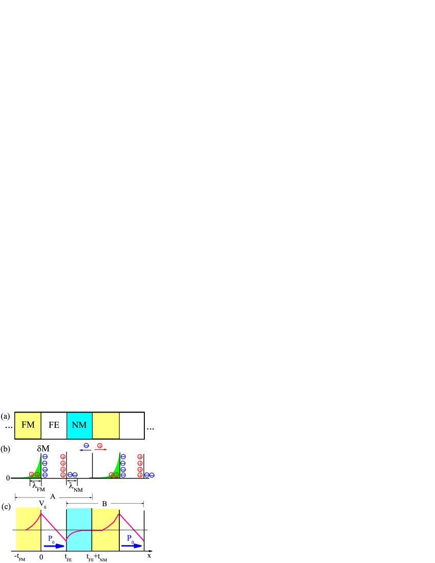
Figure 1: (Color online). (a) Schematic illustration of FM/FE/NM tri-component superlattice. (b) The distribution of charges and induced magnetization (green) calculated by our theoretical model. A and B are two different choices of the unit cell. The directions of arrows indicate the motions of positive (red) and negative (blue) charges across the boundary of the unit cell A. (c) Electrostatic potential profile.

The tri-component superlattice is illustrated in Fig.1 (a). When the FE layer is polarized, surface charges are created. These bound charges are compensated by the screening charge in both FM and NM electrodes. In the FM metal, the screening charges are spin polarized due to the ferromagnetic exchange interaction. The spin dependence of screening leads to additional magnetization in the FM electrode as illustrated in Fig.1(b). If the density of screening charges is denoted as $\eta$ and the spin polarization of screening charges as $\zeta$, we can directly express the induced magnetization per unit area as

$$\Delta M=\frac{\eta}{e}\cdot\zeta\mu_{B}.$$ (1)

As this effect depends on the orientation of the electric polarization in FE, the magnetoelectric (ME) coupling is expected.

Before starting specific calculations, let’s consider two simple cases. (1) In an ideal capacitor where all the surface charges reside at the metal (FM or NM)/FE interfaces, the density of screening charge $\eta$ reaches its maximum value, $\eta=P_{0}$, where $P_{0}$ is the spontaneous polarization of the FE. This results in a large induced magnetization ($\frac{P_{0}}{e}\cdot\zeta\mu_{B}$). (2) In half metals, there is only one type of carriers that can provide the screening. If a half metal is chosen to be the FM electrode, the screening electrons will be completely spin-polarized. In this case, a large induced magnetization is also expected, $\Delta M$= $\frac{\eta}{e}$$\mu_{B}$.

Induced Magnetization from screening charges. For simplicity, we will first consider the case of zero bias, as illustrated in Fig.1c. Here, the following assumptions are made. (1)The difference in the work function between FM and NM is ignored. (2)To screen the bound charges in FE, the charges in metal electrodes will accumulate at the FM/FE side, and there is a depletion at the NM/FE side. In this process, the total amount of charge is conserved, however, the spin density is not conserved because of the ferromagnetic exchange interaction in the FM metal.

As shown in Fig.1, the local induced magnetization, defined as $\delta M(x)=[\delta n^{\uparrow}(x)-\delta n^{\downarrow}(x)]\mu_{B}$, is a function of distance from the interface $x$. Here, $\delta n^{\sigma}(x)$ is the density of the induced screening charges with spin $\sigma$. Zhang [12] considered the FM/dielectric interface within the linearized Thomas-Fermi model and derived two coupled equations relating the local induced magnetization $\delta M(x)$ and screening potential $V_{0}(x)$,

$$\left\{{\begin{array}[]{*{20}c}{\delta M(x)=-\frac{{M_{0}/\mu_{B}}}{{1+JN_{0}}}eV_{0}(x)}\\ {\frac{{d^{2}V_{0}(x)}}{{dx^{2}}}=\frac{1}{{\lambda_{FM}^{2}}}V_{0}(x)}\\ \end{array}}\right.$$ (2)

The screening length in the FM electrode is defined as $\lambda_{FM}=\left\{{\frac{{e^{2}N_{0}}}{\varepsilon_{0}}\frac{{N_{0}+JN_{0}^{2}-J(M_{0}/\mu_{B})^{2}}}{{1+JN_{0}}}}\right\}^{-1/2}$, where $N_{0}=N^{\uparrow}+N^{\downarrow}$ is the total density of states, $M_{0}=(N^{\uparrow}-N^{\downarrow}$)$\mu_{B}$ can be thought of as the spontaneous magnetization, $\varepsilon_{0}$ is the vacuum dielectric constant and $J$ is the strength of the ferromagnetic exchange coupling in the FM layer.

We solve the above equations for our unit cell and obtain

$$V_{0}(x)=\left\{{\begin{array}[]{*{20}c}{\frac{{\eta\lambda_{FM}}}{{\varepsilon_{0}}}e^{x/\lambda_{FM}},}&{-t_{FM}\leq x\leq 0;}\\ {-\frac{{\eta\lambda_{NM}}}{{\varepsilon_{0}}}e^{-(x-t_{FE})/\lambda_{NM}},}&{t_{FE}\leq x\leq t_{FE}+t_{NM}.}\\ \end{array}\begin{array}[]{*{20}c}{}\hfil\\ {}\hfil\\ \end{array}}\right.$$ (3)

where $\eta$ is the density of screening charges, $\lambda_{FM(NM)}$ is the screening length of FM(NM) electrode, and $t_{FM}$, $t_{FE}$ and $t_{NM}$ are the thickness of FM, FE and NM layer, respectively. From above equations, we see that the local induced magnetization $\delta M(x)$ decays exponentially away from the FM/FE interface. This distribution is identical to that of screening charges, because in our model the effective interaction $J$ in FM is assumed to be a constant. The total induced magnetization $\Delta M$ can be calculated by integrating $\delta M(x)$ over the FM layer,

$$\Delta M=\int_{\text{FM layer}}\delta M(x)=-\frac{{\eta M_{0}/e}}{{N_{0}+JN_{0}^{2}-J(M_{0}/\mu_{B})^{2}}}.$$ (4)

The effective spin polarization of screening electrons can then be written as

$$\zeta=-\frac{{M_{0}}}{{N_{0}+JN_{0}^{2}-J(M_{0}/\mu_{B})^{2}}}.$$ (5)

We have considered the induced magnetization in FM/FE/NM tri-component superlattice with several FM electrodes, i.e., Fe, Co, Ni and CrO₂. Detailed parameters and calculated values of $\Delta M$ are listed in Table I. The magnitude of $\Delta M$ is found to depend strongly on the choice of the FM and FE. Among the normal FM metals (Ni, Co and Fe), the largest $\Delta M$ is observed in Ni for its smallest $J$ and highest spontaneous spin polarization $M_{0}/\mu_{B}N_{0}$. On the other hand, we also predict a large $\Delta M$ for the 100% spontaneous spin polarization in half-metallic CrO₂.

Table 1: Parameters extracted from band structures of Ni, Co, Fe from Ref.[12], CrO₂ from Ref.[22]. Here, $\Delta M$ is the value at $V_{a}$=$V_{C}$, where $V_{a}$ is the applied bias and $V_{C}$ is the coercive bias.

FM	$J$ (eV$\cdot$nm3)	$N_{0}$ (eV-1$\cdot$nm-3)	$M_{0}/\mu_{B}N_{0}$	$\lambda_{FM}$ (Å)	$\Delta M$ ($\mu_{B}$$\cdot$nm-2)	$\tau$ (G cm/V)
Ni	0.65	1.74	-79.3%	0.9	-0.280	0.015
Co	1.25	0.89	-58.4%	1.5	-0.126	0.004
Fe	2.40	1.11	56.8%	1.3	0.078	0.003
CrO2	1.8	0.69	100%	1.7	0.323	0.010

To confirm the validity of our model, we perform first-principles calculations of the Fe/FE/Pt superlattice [23]. The calculations are within the local-density approximation to density-functional theory and are carried out with VASP [24]. We choose BaTiO₃ (BTO) and PbTiO₃ (PTO) for the FE layer. Starting from the ferroelectric P4mm phase of BTO and PTO with polarization pointing along the superlattice stacking direction, we perform structural optimization of the multilayer structures by minimizing their total energies. The in-plane lattice constants are fixed to those of the tetragonal phase of bulk FEs. Fig. 2 shows the calculated induced magnetic moment relative to that of bulk Fe near the Fe/BTO interface when the polarization in BaTiO₃ points toward the Fe/BTO interface. It is evident that the induced moments decay exponentially as the distance from the interface increases. This result is in line with our model for the magnetization accumulation in the FM at the FM/FE interface. A numerical fitting of the exponential function yields a screening length of $\sim 0.7$ Å  for the Fe/BaTiO₃/Pt structure. This value is comparable to the screening length parameters calculated using the theoretical model as shown in Table I.

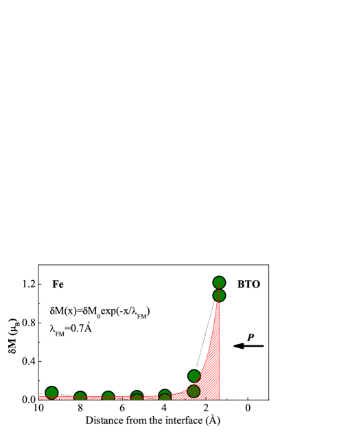
Figure 2: (Color online). Layer-resolved induced magnetic moment of Fe near the interface between Fe and BaTiO₃ in the Fe/BaTiO₃/Pt superlattice. Solid line is the fitted exponential function for the induced moment as a function of the distance from the interface.

Using our theoretical model we also calculate the ME coupling coefficient $\tau$, which is defined as the ratio of the magnetization change 2$\mu_{0}\Delta M/\lambda_{FM}$ to the coercive field $V_{C}/(l*t_{FE})$, where $V_{C}$ is the coercive voltage and $l$ is the number of the unit cell. The $\tau$ values listed in Table I reach as large as 0.015 G cm/V in Ni. For comparison, $\tau$ of about 0.01 G cm/V arising from the chemical bonding between Fe and Ti atoms is predicted for the Fe/BaTiO₃ bilayer [11]. The ME coefficient measured in epitaxial BiFeO₃-CoFe₂O₄ columnar nanostructures [10] is also of 0.01 G cm/V. We should point out that in our calculation the coercive field is assumed to be 200 kV/cm, if we choose the coercive field of 10 kV/cm same as Ref. [11], $\tau$ will be 20 times larger than those listed in Table I. Therefore, the ME effect arising from spin-dependent electron screening in FM/FE/NM tri-component superlattice can be much larger than in other composite multiferroics.

What is the source of this large ME effect? In fact, the magnetoelectric effect discussed in this letter is not the usual bulk magneto-electric coupling at all. Spontaneous electric polarization in FE results in the induced surface charge. In turn, this produces the screening charges of density $\eta$. These screening charges are polarized with the polarization $\zeta$. Therefore, it is the amount of screening charges and polarization that determine the magnitude of the ME effect ($\Delta M$ and $\tau$). If we expand the induced magnetization $\Delta M$ in Eq.(4) as power series in order parameters $P_{0}$ and $M_{0}$ (spontaneous polarization and magnetization), we obtain

$$\Delta M\propto P_{0}M_{0}+\text{high-order terms in P${}_{0}$ and M${}_{0}$}$$ (6)

The higher order terms in Eq.(3) vanish exactly in the following limiting case: the screening length $\lambda_{FM}\rightarrow 0$ and spin polarization $\zeta\rightarrow\pm 100\%$. In general, the leading term in Eq.(6) is linear, which is consistent with the computational result of Ref.[13]. It is also clear that this effect depends on the magnetization of the ferromagnetic metal.

First-principle calculations confirm the central conclusion that the ME coupling in the tri-component system is linear in polarization of FE. We compare a superlattice with BTO and that with PTO. The induced magnetization difference is 3.6 times larger in the the case of PTO. This ratio is almost exactly that of the bulk spontaneous polarization of BTO and PTO.

Electric control of magnetization. So far, we have discussed the magnetoelectric coupling effect in the case of no external bias. A natural question is what happens to $\Delta M$ when external bias $V_{a}$ is applied. In this case, the electric polarization $P$ will have two parts: the spontaneous polarization $P_{0}$ and induced polarization. The equation determining $P$ is obtained by minimizing the Free energy. From the continuity of the normal component of the electric displacement, we find equation relating $\eta$ and $P$: $\eta=(\frac{P\cdot t_{FE}}{\varepsilon_{FE}}+\frac{V_{a}}{l})/(\frac{\lambda_{FM}+\lambda_{NM}}{\varepsilon_{0}}+\frac{t_{FE}}{\varepsilon_{B}})$. Here, $\varepsilon_{FE}$ is the dielectric constant of the FE layer. These two equations need to be solved self-consistently. The value of $\eta$ at a given bias can then be calculated and the induced magnetization $\Delta M$ is given by Eq.(4).

The free energy density $F$ includes contributions from the FE layer, FM layer and FM/FE interface and takes the form

$$F=\frac{{t_{FE}\cdot F(P)+t_{FM}\cdot F(M)+F_{I}(P,M)}}{{t_{FE}+t_{FM}+t_{NM}}}.$$ (7)

$M$ is the magnetization of the bulk ferromagnet, and here $M$=$M_{0}$ because of zero external magnetic field. The interface energy $F_{I}(P,M)$ is the sum of the electrostatic energy and magnetic exchange energy of the screening charges

$$F_{I}(P,M)=\frac{{(\lambda_{FM}+\lambda_{NM})}}{{2\varepsilon_{0}}}\eta^{2}+\frac{{J}}{{2\mu_{B}^{2}}}(M+\Delta M)\cdot\Delta M.$$ (8)

For FE, the free energy density $F(P)$ can be expressed as $F(P)=F_{P}+\alpha_{P}P^{2}+\beta_{P}P^{4}+\int_{0}^{P}{E_{B}dP}$, where $F_{P}$ is the free energy density in the unpolarized state. $\alpha_{P}$ and $\beta_{P}$ are the usual Landau parameters of bulk ferroelectric. $E_{B}$ is the depolarization field in the FE film. Similarly, $F(M)$ can be expanded as a series in order parameter $M$, i.e., $F(M)=F_{M}+\mu_{M}M^{2}+\nu_{M}M^{4}$, where $F_{M}$ is the free energy density of bulk ferromagnet, $\mu_{M}$ and $\nu_{M}$ are the Landau parameters of bulk ferromagnet. The calculated induced magnetization as function of applied bias is shown in Fig.3. Clearly, the electrically controllable magnetization reversal is realized.

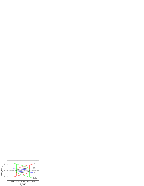
Figure 3: (Color online) $\Delta M$ versus $V_{a}/l$ for different ferromagnetic metal electrodes. $V_{a}$ is the applied bias and $l$ is the number of the unit cell. Here, the thickness of FE layer is 3 nm. However, a thicker FE layer can be used to avoid the possible electron tunneling effect.

To discuss the macroscopic properties of the electric control of magnetization, we analyze the magnetoelectric coupling energy in our tri-component superlattice. For the macroscopic average polarization to be represented by the electric polarization obtained for a unit cell, this cell needs to be chosen with special care [25]. Therefore, in the following calculation of total free energy, unit cell $\bf B$ in Fig.1(b) is chosen, and

$$\bar{P}=\frac{{P\cdot t_{FE}+\eta(t_{FM}+t_{NM})}}{{t_{FE}+t_{FM}+t_{NM}}}.$$ (9)

The macroscopic average magnetization $\bar{M}$ is

$$\bar{M}=\frac{{M\cdot t_{FM}+\Delta M}}{{t_{FE}+t_{FM}+t_{NM}}}.$$ (10)

Considering the lowest order term of the magnetoelectric coupling, $\bar{P}$ and $\bar{M}$ can be expanded as $\bar{P}=c_{p}P+c_{p}^{\prime}PM^{2};\bar{M}=c_{m}M+c_{m}^{\prime}PM$. Therefore, the total free energy (Eq.(7)) can be expressed as the power series of $\bar{P}$ and $\bar{M}$, $F(\bar{P},\bar{M})=F_{0}+\alpha\bar{P}^{2}+\beta\bar{P}^{4}+\mu\bar{M}^{2}+\nu\bar{M}^{4}+\chi\bar{P}\bar{M}^{2}+\cdots.$ We would like to point out that biquadratic ME coupling $\bar{P}^{2}\bar{M}^{2}$ is easily achievable, but is usually weak and is not electrically controllable. However, because of the naturally broken inversion symmetry, the large ME coupling $\bar{P}\bar{M}^{2}$ is possible in our tri-component structure.

The ME coupling in FM/FE/NM superlattices may be observed experimentally and may have practical applications. Though the net additional magnetization of each FM/FE/NM unit cell is small, stacking several of them in a superlattice will result in a large overall magnetization. From Eq.(10), with a thinner metallic electrode, the ME effect will be larger, as long as the thickness of metallic electrodes are larger than the screening length, which is easy to achieve.

To summarize, expanding upon the theory of spin-dependent screening[12], we develop a theory of additional magnetization in tri-component superlattice. We show that the additional magnetization can be electrically controlled, and is linear in FE polarization. The latter can be switched if the coercive voltage of the ferroelectric is reached. We demonstrate that an asymmetric FM/FE/NM structure has practical advantages over previously discussed symmetric structure.

Acknowledgments: TC and QN were supported by DOE (DE-FG03-02ER45985), NSF(DMR0906025), Welch Foundation (F-1255), and NSFC (10740420252). SJ were supported by K. C. Wong Education Foundation, Hong Kong and China Postdoctoral Science Foundation. JL,NS and AAD were supported by the Office of Naval Research (N000 14-06-1-0362) and Texas Advance Computing Center.

References

- [1] M. Fiebig, J. Phys. D 38, R123 (2005).
- [2] N. A. Hill, J. Phys. Chem. 104, 6694, (2000).
- [3] W. Eerenstein, N. D. Mathur, and J. F. Scott, Nature (London) 442, 759 (2006).
- [4] S.-W. Cheong and M. Mostovoy, Nature Materials 6, 13 (2007).
- [5] R. Ramesh and N. A. Spaldin, Nature Materials 6, 21(2007).
- [6] Y. Tokura, J. Magn. Magn. Mater. 310, 1145 (2007).
- [7] A. Malashevich and D. Vanderbilt, Phys. Rev. Lett. 101, 073210 (2008).
- [8] C. J. Fennie and K. M. Rabe, Phys. Rev. Lett. 97, 267602 (2006).
- [9] H. Zheng, J. Wang, S. E. Lofland, Z. Ma, L. Mohaddes-Ardabili, T. Zhao, L. Salamanca-Riba, S. R. Shinde, S. B. Ogale, F. Bai, D. Viehland, Y. Jia, D. G. Schlom, M. Wuttig, A. Roytburd, R. Ramesh1, Science 303, 661 (2004).
- [10] F. Zavaliche, T. Zhao, H. Zheng, F. Straub, M. P. Cruz,? P.-L. Yang, D. Hao, and R. Ramesh, Nano Letters 5, 1793 (2005).
- [11] C. G. Duan, S. S. Jaswal, and E. Y. Tsymbal, Phys. Rev. Lett. 97, 047201 (2006).
- [12] S. F. Zhang, Phys. Rev. Lett. 83, 640 (1999).
- [13] J. M. Rondinelli, M. Stengel and N. A. Spaldin, Nature Nanotechnology 3, 46 (2008).
- [14] C.G. Duan, J.P. Velev, R.F. Savirianov, Z.Q. Zhu, J.H. Chu, S.S. Jaswal, and E.Y. Tsymbal, Phys. Rev. Lett. 101, 137201 (2008).
- [15] T. Maruyama, Y. Shiota, T. Nozaki, K. Ohta, N. Toda, M. Mizuguchi, A. A. Tulapurkar, T. Shinjo, M. Shiraishi, S. Mizukami, Y. Ando, and Y. Suzuki, Nature Nanotechnology 4, 158 (2009).
- [16] P. Batra and B. B. Silverman, Solid State Commun. 11, 291 1972; P. Wurfel and I. P. Batra, Ferroelectrics 12, 55 (1976).
- [17] J. Junquera and P. Ghosez, Nature 422, 506 (2003).
- [18] N. Sai, A. M. Kolpak and A.M. Rappe, Phys. Rev. B 72 020101 (2005)
- [19] E. Y. Tsymbal and H. Kohlstedt, Science 313, 181 (2006).
- [20] M. Ye. Zhuravlev, R. F. Sabirianov, S. S. Jaswal, and E. Y. Tsymbal1, Phys. Rev. Lett. 94, 246802 (2005).
- [21] S. Ju, T. Y. Cai, G. Y. Guo, and Z. Y. Li, Phys. Rev. B 75, 064419 (2007).
- [22] A. M. Bratkovsky, Phys. Rev. B 56, 2344 (1997).
- [23] J.K. Lee, N. Sai, T.Y. Cai, Q. Niu, and A. A. Demkov, in preparation.
- [24] The DFT calculations were performed within the local spin density approximation as implemented in VASP (G. Kresse and J. Furthmüller, Phys. Rev. B 54 11169 (1996)). We have used a planewave energy cutoff of 600 eV and a 6x6x1 centered -point mesh for the integration of the Brillouin zone.
- [25] The polarization (i.e. computed via the Berry phase) is of course cell independent. There is, however, one ”natural” cell for which the macroscopic average polarization can be represented by the cell dipole. That fact is used in Eq.(9) and unit cell is chosen. In one-dimensional case, assuming electric current is a non-spinor and choosing an appropriate gauge, the fundamental laws of electrodynamics are (1’) and (2’). Here, is the electric polarization and is the charge density. Choosing an appropriate unit cell, the macroscopic average polarization can be represented by the cell dipole, i.e., (3’), where and are the boundaries of the unit cell. Combing Eq.(3’) with Eqs.(1’) and (2’), it is found that the left hand of Eq.(3’) is , while the right hand of Eq.(3’) is the sum of and . Thus, only when the condition of no charge exchange between the neighboring unit cells is satisfied, i.e., , the macroscopic average electric polarization can be represented by the cell dipole. Unit cell isn’t the appropriate one because the current will develop across it during polarization switching.