Water-waves modes trapped in a canal by a body
with the rough surface
Abstract
The problem about a body in a three dimensional infinite channel is considered in the framework of the theory of linear water-waves. The body has a rough surface characterized by a small parameter while the distance of the body to the water surface is also of order . Under a certain symmetry assumption, the accumulation effect for trapped mode frequencies is established, namely, it is proved that, for any given and integer , there exists such that the problem has at least eigenvalues in the interval of the continuous spectrum in the case . The corresponding eigenfunctions decay exponentially at infinity, have finite energy, and imply trapped modes.
AMS Subject Classification: 76B15, 35P20.
Key words and phrases: trapped modes, eigenvalues, asymptotic analysis.
1 Introduction
1.1 Statement of the problem.
Let be a domain on the plane bounded by the line interval and the smooth simple curve inside the lower half-plane which meets at the points with the angles (see Fig. 1, a).
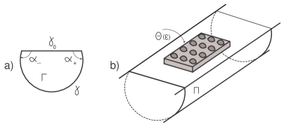
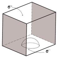
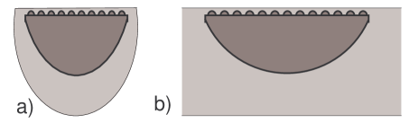
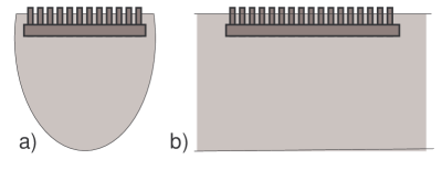
The three-dimensional canal with the horizontal plain surface contains the finite body (see Fig. 1, b). The shape of the body depends on the small parameter so that its upper surface is rough with periodic fine knobs and/or caverns of size (see Fig. 2 with the three-dimensional image and Fig. 3 with the two-dimensional cross-sections). The body is submerged in the superficial region and the mean distance from to the upper surface of is of order as well. There is no geometrical restriction on the bottom of but the upper rough horizontal part of the boundary restricts from below a finite thin rectangular plate-shaped part of the near-surface water layer (see Fig. 4)
| (1.1) |
In other words, the upper straight base of the plate belongs to the horizontal surface of water while the lower base of a fine periodic structure reposes upon the boundary of the body.


Although further results are valid for Lipschitz surface (see Section 4), we assume in the presentation that this surface is smooth enough though. The assumption crucially simplifies rather cumbersome calculations in Sections 2.4 and 2.5.
To describe the periodic structure of the plate more precisely, we introduce the periodicity cell such that
where is a rectangle ( and We introduce another rectangle
| (1.2) |
and assume that the sizes are in the relation
where and are large positive integers. We then set
| (1.3) |
| (1.4) |
where is a multi-index and The domain , i.e., the interior of the closed set (1.3) is but a thin plate composed from the large number of small periodicity cells (1.3). We do not exclude the case when and imply parallelepipedes of sizes and respectively (cf. [1]).
Notice that it is convenient to use different notation for the same Cartesian coordinate system namely, in the canal and in the plate while are coordinates on the cross-section of and are coordinates on the upper base of
In the canal with the submerged body we consider the spectral problem of the linearized water-wave theory
| (1.5) |
| (1.6) |
| (1.7) |
(see, e.g., monographs [2, 3, 4] for physical and mathematical background). Here is the Laplace operator, and , while is the derivative along the outward normal, in particular, on Furthermore, is the velocity potential and the spectral parameter, proportional to square of frequency of harmonic oscillations in the canal.
In addition to the smoothness assumptions introduced above, the whole boundary is Lipschitz. Hence, the normal and the Neumann (1.6) and the Steklov (1.7) boundary conditions are defined properly for almost all However, the gradient can gain singularities, e.g., at edges on the boundary and in Section 1.3 we give a precise definition of an operator for problem (1.5)-(1.7) in the Sobolev space In this framework, being interested to detect trapped modes, i.e., solutions with the exponential decay as we need not to supply the problem with any radiation condition at infinity. We again refer to [2, 3, 4] for formulation of these radiation conditions in similar geometrical situations.
1.2 The trapped modes frequencies
In this paper we seek for trapped modes, i.e., solutions of problem (1.5)-(1.7) with the finite energy and, therefore, the exponential decay at infinity. Such solutions have been a goal in many investigations (see [5]-[13] and review [14] for much more extensive list of references). In the sequel we detect the accumulation effect of trapped mode eigenfrequencies, namely, assuming the geometrical parameter sufficiently small, we find out any prescribed number of eigenvalues on the given small interval of the continuous spectrum in problem (1.5)-(1.7). We make use of the following issues:
-
•
The artificial Dirichlet boundary conditions on the plane
-
•
Asymptotic analysis for eigenvalues of a spectral problem in the thin finite domain
-
•
The operator formulation of the problem in Hilbert space.
-
•
The max-min principle.
Let us outline these issues.
First, the artificial Dirichlet boundary conditions on the plane of geometrical symmetry permit to create a positive threshold in the modified spectral problem so that the continuous spectrum covers the ray but leaves the gap for the discrete spectrum. This trick was proposed in [15] for detecting trapped modes in a strip with a symmetric obstacle for the Helmholts equation with the Neumann boundary conditions.
Second, as a subsidiary problem, we investigate sloshing mode eigenfrequencies in the artificially constructed thin finite layer of water (see formula (1.1) and Fig. 4 where it is demonstrated how the plate-shaped layer is cut off and separated by the body In other words, we consider the auxiliary Steklov spectral problem
| (1.8) |
| (1.9) |
| (1.10) |
The asymptotic analysis of (1.8)-(1.10) is rather standard (cf. [16, 17, 18] and others). However, a new effect is observed in Theorem 7: each entry of the monotone unbounded eigenvalue sequence in problem (1.8)-(1.10)
| (1.11) |
becomes infinitesimal when Namely, the eigenvalues belong to the interval if with a certain
It suffices to prove that the point spectrum of problem (1.5)-(1.7) in the interval contain at least eigenvalues. This task is fulfilled by applying the max-min principle (see, e.g., [21, Theorem 10.2.2]) to the operator formulation [1] of the problem (respectively the fourth and third issues in the above list). We emphasize that the lateral side of the plate is supplied with the Dirichlet conditions (that is why we call (1.8)-(1.10) the Steklov spectral problem while the complete analogy with sloshing modes is dubious). We again use the geometrical symmetry and reduce the problem (1.8)-(1.10) onto the subdomain Imposing the Dirichlet condition on the artificial boundary we keep the concentration property for eigenvalues of the Steklov problem in The Dirichlet conditions and the inclusion permit for the extension of the corresponding eigenfunctions by zero from onto the set
| (1.12) |
These extended eigenfunctions are taken as trial functions in the max-min principle which ensure that, for any the point spectrum of the problem in contains an eigenvalue
1.3 Preliminary description of results.
The operator formulation of problem (1.5)-(1.7) given in Section 3.2 permits to deal with its spectrum within the spectral theory of self-adjoint operators in Hilbert space. If is a complex number and then evidently, the inhomogeneous problem (1.5)-(1.7) with data in the Lebesgue spaces and admits a unique generalized solution in the Sobolev space (see the integral identity (3.3) and cf. [19]). This fact means that implies the resolvent set of the operator of problem (1.5)-(1.7). In Section 3.3 we show that the closed real positive semi-axis is covered with the continuous spectrum of (Lemma 8).
Under the assumption
| (1.13) |
which requires the symmetry of domain (1.13) with respect to the middle plane of the canal (cf. Fig. 3, a, where the dotted line indicates the symmetry axis of the transverse cross-section of the canal), we treat the restriction of the operator onto the subspace
| (1.14) |
and associate with the operator a problem obtained from (1.5)-(1.7) by restricting onto a half of the domain for definiteness on the right half (1.12), and supplied with the artificial boundary condition
| (1.15) |
on the artificially generated surface Such the restricted problem is further referred as the problem (1.5)-(1.7), (1.15) on the domain
In Section 3.3, owing to the Dirichlet boundary conditions (1.15), we find out a threshold , depending only on the cross-section , such that the continuous spectrum of implies the ray while the segment contains only the discrete spectrum of
Note that the odd extension of an eigenfunction of the problem in becomes an eigenfunction of the problem in corresponding to the same eigenvalue Based on the above-mentioned observations, we prove in Section 3.4 the main result of the paper.
Theorem 1
Under the geometrical assumptions (1.1), (1.4) and (1.13), for any and there exists such that in the case problem (1.5)-(1.7) has at least eigenvalues in the interval The corresponding eigenfunctions decay exponentially at infinity and, therefore, imply so-called trapped modes in the linear theory of water-waves.
We emphasize that the eigenvalues in Theorem 1 lie in the continuous spectrum of the operator
Our approach does not require any other global geometry assumption on the shape of the body whilst the symmetric cross-section of the canal is arbitrary. Moreover, any given large number of trapped modes with the frequencies in any preadjusted small interval can be obtained.
2 Asymptotics of eigenvalues of the spectral problem in the thin domain
2.1 Formal asymptotic analysis.
We employ the standard asymptotic expansions of solutions in thin domains (see, e.g., [20],[18, Ch.7])
| (2.1) |
where and are a number and functions to be determined and stands for the ”fast” variables
| (2.2) |
We insert formulae (2.1) into equation (1.8) and the boundary conditions (1.9) and gather coefficients on similar powers of the small parameter Since the derivatives in and of the function are equal to
respectively, we obtain the following problems on the periodicity cell with the parameter
| (2.3) |
| (2.4) | ||||
| (2.5) | ||||
Here is the outward unit normal to the upper and lower bases of the cell (see Fig. 5 and compare with Fig. 4), on and so that on
Problems (2.3)-(2.5) are also supplied with the periodicity conditions on the opposite lateral sides of the cell (a couple of them is overshadowed in Fig. 5). Note that is the surface which completes these sides and the rectangular ”cover” up to the whole boundary We do not write explicitly the periodicity conditions but always deal with solutions which are periodic in the variables
Equations (2.3) hold true because does not depend on the fast variables in (2.2). Since, evidently,
problem (2.4) admits a solution in the form
| (2.6) |
where and raise the standard asymptotic corrector in the theory of homogenization (see, e.g., [16, 17]). Namely, is a (periodic in ) solution of the model problem
| (2.7) |
We emphasize that, by definition, on and, according to the assumed smoothness of the lower base of the cell, the periodic functions are infinitely differentiable.
We now consider problem (2.5). Note that the factor in the representation (2.1) of the eigenvalue was introduced to fulfil the goal: the main asymptotic term of the right-hand side in the spectral boundary condition (1.9) of the Steklov type comes into a problem for the asymptotic term in the expansion for the eigenfunction
The compatibility condition in problem (2.5) reads
| (2.8) |
where meas is the volume of the cell and the area of the cover Owing to (2.6), equality (2.8) can be rewritten in the form
| (2.9) |
Here is a matrix of size with the entries
| (2.10) | ||||
By is denoted the natural inner product in the Lebesgue space . The vector functions and are linear independent because and are periodic in Thus, the matrix with entries (2.10) implies a Gram matrix, i.e. it is positive definite and symmetric and, therefore, is a second order elliptic differential operator.
2.2 Spectrum of the resultant problem.
Problem (2.9), (2.11) can be reformulated as the integral identity [19]
| (2.12) |
the left-hand side of which implies an inner product in the subspace of functions satisfying condition (2.11). Owing to the compact embedding spectrum of the operator, associated with the bi-linear form (see [21, §10.1]), is descrete and form the positive monotone unbounded sequence
| (2.13) |
where eigenvalues are repeated according to their multiplicity.
The corresponding eigenfunctions can be subject to the normalization and orthogonality condition
| (2.14) |
where , and is Kronecker’s symbol. The first eigenvalue is simple due to the strong maximum principle.
An affine transform of the coordinate system turns the differential operator on the left of (2.9) into the Laplace operator while the rectangle becomes a parallelogram. A harmonic function, which has the finite Dirichlet integral and vanishes at both sides of an angle with the opening possesses the worst singularity where is the polar coordinate system and (see, e.g., [22], and introductory chapters in [23], [24]). Thus, the theory of elliptic boundary value problems in domains with piecewise smooth boundaries, especially, a result in [25], ensures the following assertion.
Lemma 2
Recall the definition of the Hölder norm
| (2.16) |
2.3 Operator formulation of the problem in
Aiming to justify asymptotic expansions constructed in Section 2.1, we endow the Sobolev space
| (2.17) |
with the specific inner product
| (2.18) |
In the obtained Hilbert space we introduce the operator by the formula
| (2.19) |
This operator is positive continuous and symmetric, therefore, self-adjoint. It is compact due to the compactness of the embedding The norm of is less than Thus, the spectrum of is descrete and forms the positive infinitesimal sequence
| (2.20) |
where eigenvalues are listed according to their multiplicity and again the first eigenvalue is simple by virtue of the strong maximum principle. The corresponding eigenfunctions can be subject to the normalization and orthogonality conditions
| (2.21) |
Remark 3
The variational formulation of problem (1.8)-(1.10)
| (2.22) |
is equivalent to the abstract equation
| (2.23) |
with the new spectral parameter
| (2.24) |
Formula (2.24) relates only the descrete spectra (2.18) and (1.11). Although the operator has the infinite-dimensional kernel this kernel does not influence the spectrum of problem (2.12) because
Justification of asymptotics is based in the next sections on the following classical result known as the lemma on ”almost eigenvalues and eigenfunctions”, a proof can be found in [26] and [21].
Lemma 4
Let and satisfy
Then at least one eigenvalue of the operator verifies the inequality
Moreover, for any , there exist coefficients such that
where means summation over all eigenvalues of the operator in the segment and are corresponding eigenfunctions under condition (2.21).
2.4 Approximation solutions.
According to (2.1) and (2.24), we take
| (2.25) |
| (2.26) |
as an approximate solution of the spectral abstract equation (2.23). In (2.25) is an eigenvalue of the resultant problem with multiplicity i.e.,
| (2.27) |
in the sequence (2.13), is a smooth cut-off function on which is equal to outside the neighborhood of and vanishes in the vicinity of e.g.,
| (2.28) |
Furthermore, and are eigenfunctions of problem (2.9), (2.11) corresponding to and verifying conditions (2.14). In other words, formulae (2.25), (2.26) deliver different approximation solutions of (2.23).
We proceed with calculation of the inner products here and in the sequel Since and
we readily obtain
|
|
Moreover,
and analogously
These inequalities allow to estimate directly certain terms on the right-hand side of the equality
|
|
and conclude that
| (2.29) |
The formula
| (2.30) |
for the integral
follows from the next lemma where it is necessary to put
Note that is the exponent in Lemma 2 and formula (2.10) is used to detect the subtrahend on the left of (2.30). The following result is known (cf. [16, 17]) so that we only adapt a standard proof for the Hölder continuous multiplier in the integrand.
Lemma 5
Let and
| (2.31) |
Then
| (2.32) |
2.5 Calculating the discrepancy
According to (2.33), we obtain
| (2.34) |
for a small Thus, by virtue of (2.25), (2.26), (2.19), (2.18), we have
| (2.35) | ||||
where the supremum is calculated over all such that . Furthermore,
| (2.36) | ||||
To examine this expression we need auxiliary inequalities.
Lemma 6
-
1.
Let and
(2.37) where
and is extended by zero from onto the thin periodic infinite layer. Then the inequality
(2.38) holds where dist Moreover,
(2.39) -
2.
A function meets the relation
(2.40) Here all constants depend on neither nor
Proof. First of all, we have
| (2.41) | ||||
where
Second,
where are the opposite lateral faces of the periodicity cell (see Fig. 5). Now repeating calculation (2.41) yields the estimate of in (2.38).
The support of function (2.37) lies in the rectangle Thus, integrating the one-dimensional Hardy inequality
and using the completion argument bring the necessary estimate of the first norm in (2.38).
Dealing with the first norm in (2.39), we compute
|
|
(2.42) |
For the second norm in (2.39), we need to replace in (2.42) the integration set by and As a result, the bound changes for
Inequality (2.40) is a direct consequence of estimates (2.38), (2.39) together with the evident relations and
Now we are in position to simplify expression (2.36) and, neglecting inessential terms and changing for , to derive that
|
|
(2.43) |
We start with the simplest term
Owing to (2.7), we here have at and, hence,
|
|
(2.44) |
For the first term (with ), we readily used the Schwarz inequality. For the second term (with ), we took into account that on supp and applied estimate (2.40). For the third term (with ), we used estimate (2.39).
Similar argument works for the last term in (2.36). Recalling boundary conditions in problem (2.7) for the asymptotic correctors we, indeed, obtain
|
|
and, therefore,
|
|
(2.45) |
Here we applied inequalities (2.40), (2.15), (2.39) while taking into account the obvious relations
Since is a harmonics, the first term in the sum vanishes. We now list down estimates permitting to neglect some other terms:
|
|
(2.47) |
Here we have applied the same arguments as above.
Inequalities (2.47) help to estimate all terms in (2.46) with exception of the first subtrahend on the left of (2.43). Other two subtrahends were exhibited in (2.45) and (2.44); hence, relation (2.43) is verified.
Similarly to the proof of Lemma 5, we now consider the integrals over the cells and their bases and namely,
|
|
(2.48) |
Freezing here the argument at the mass center of the rectangle we perform integration in and, recalling calculation (2.10), we obtain that expression (2.48) turns into the expression
which vanishes because is an eigenpair of problem (2.9), (2.11). The error of the freesing procedure does not exceed
| (2.49) |
while the weight factor comes from inequality (2.15) with Since
|
|
quantity (2.49) may be bounded from above by
2.6 The theorem on asymptotics of eigenvalues.
Owing to (2.50), Lemma 4 delivers an eigenvalue of the operator such that
| (2.51) |
By (2.24), we have and, hence,
| (2.52) |
This particularly gives
Thus, with a small and , we obtain
and, according to (2.52),
| (2.53) |
Theorem 7
Proof. It suffices to compute a bound for the number of eigenvalues in (2.53). Employing again Lemma 4, we set where is taken from (2.50). Then, for , we get coefficients such that
| (2.54) |
where is the list of all eigenvalues in (2.18) which meet the inequality
| (2.55) |
Recall that the coefficient columns are of unit length. Moreover, by (2.33) and (2.21), we have
|
|
Thus, for small and , the columns are linear independent in so that Since inequality (2.55) is just of the same kind as inequality (2.51) which has resulted in (2.53), the proof of the theorem is completed.
3 Spectra of the problems
3.1 Variational formulation of problems.
Let denote the Sobolev space equipped with the specific norm
| (3.1) |
and the corresponding inner product (cf. (2.22)). We also introduce the weighted Sobolev space as the completion of (infinitely differentiable functions with compact supports) with respect to the norm
| (3.2) |
where and This space consists of all functions with the finite norm (3.2). Clearly, If , a function decays exponentially as but the space with includes functions with a certain exponential growth at infinity.
The standard formulation [19] of the spectral problem (1.5)-(1.7) reads: to find and such that
| (3.3) |
For a fixed we also consider the integral identity
| (3.4) |
serving for the inhomogeneous problem (1.5)-(1.7) while is a linear functional in the Hilbert space A generalized solution of problem (1.5)-(1.7) in the weighted space implies a function such that
| (3.5) |
where Formally, (3.5) is derived from (3.4) by changing the test function for the product Notice that the linear space is dense in with any weight index
By the definition of the weighted norm (3.2), in case Hence, and stand in (3.5) for extensions of the natural inner products in and up to the duality between proper weighted Lebesgue spaces.
Let and while so that as well. Then, if is a solution of problem (3.5), belongs to and is a solution of problem (3.4) with an exponential decay at infinity. Viceversa, in the case a solution of problem (3.4), where , becomes a solution of problem (3.5) in
Under the symmetry assumption (1.13), the same definition works for the problem posed on the set (1.12) with the artificial Dirichlet conditions (1.15). We use the notation and for the function space (1.14) and the similar weighted space of odd functions. Moreover, integral identities for this problem on are refereed as the identities (3.3), (3.4) and (3.5) restricted onto the subspaces and , respectively.
3.2 The operator formulation of problems.
In the Hilbert space with the inner product , generated by norm (3.1), we introduce the operator by the formula
| (3.6) |
(cf. formulae (2.18) and (2.19) in the domain ). This operator is continuous with the unit norm, positive and self-adjoint but not compact because the surface is unbounded. Thus its spectrum lies on the segment of the real axis and its essential spectrum does not reduce to the single point (see, e.g., [21, Ch. 10]).
The restriction of on the subspace is denoted by Clearly, acts from into . If is an eigenvalue of the operator with the eigenfunction analogously to (2.24),
| (3.7) |
is an eigenvalue of problem (3.3) restricted on i.e., of the operator Moreover, the odd extension of the function over the plane becomes an eigenfunction of problem (3.3) (and problem (1.5)-(1.7) on ) corresponding to the same eigenvalue (3.7). This observation will be a tool to prove Theorem 1, the main result of the paper.
3.3 Continuous spectra.
Clearly, the point is an eigenvalue of the operator with the infinite-dimensional eigenspace
| (3.8) |
A similar conclusion holds true for the operator
Lemma 8
The segment is filled with the continuous spectrum of the operator
Proof. The assertion follows from general results [27] (see also §5.1 in [23]). For the reader convenience, we show here shortly how to construct a singular Weyl sequence for any so that belongs to the essential spectrum of Since the operator of problem (3.5) regarded as the mapping is Fredholm for a sufficiently small negative (see [27], [23, Theorem 5.1.4] and comments on the model problem (3.9) below), the kernel of this operator at regarded as the mapping , is finite-dimensional. Thus, any point of the essential spectrum lies in the continuous spectrum of
Let consider the model problem on the cross-section of the canal namely
|
|
(3.9) |
Problem (3.9) is obtained by the Fourier transform from the problem of type (1.5)-(1.7) in the cylindrical channel while is the dual Fourier variable for Let be an unbounded operator in associated (see [21, Ch.10]) with the bi-linear form
| (3.10) |
This operator is self-adjoint and bounded from below. Its domain belongs to Since the embedding is compact, and
|
(3.11) |
Theorems 10.1.2, 10.1.5, 10.2.4 in [21] ensure that the spectrum of is descrete and form the eigenvalue sequence
| (3.12) |
while is a continuous, strictly monotone decreasing negative function. The first eigenvalue is simple due to the maximum principle and is imaginary. Let be the first eigenfunction of problem (3.9). We set
| (3.13) |
where is a normalization factor, is the plateau function in Fig. 6,
| (3.14) |
and is a cut-off function, for and for The function is equal to one on the segment
| (3.15) |
and both functions (3.14) and (3.13) vanish for
| (3.16) |

In the case we simply set We choose an integer such that and obtain
|
|
(3.17) |
We fix such that the last expression equals A similar calculation shows that is bounded from above uniformly in . The supports of the functions and with are disjoint due to (3.16) Hence, converges to zero weakly in as and implies a Weyl sequence provided
| (3.18) |
We have
Here the supremum is calculated over all such that By the definition of and as a solution of problem (3.19), function (3.13) satisfies the boundary condition (1.7) on and it is harmonic on a part of the cylinder determined by relation (3.15). Thus, the expression (3.19) reduces to integral over the finite cylinders
and, therefore, it does not exceed The proof is completed.
The model problem on the cross section of cylinder (1.12)
| (3.19) | ||||
corresponds to the operator of problem (3.3) restricted on Here and the curves compose the boundary of
First of all, we put and denote by the first eigenvalue of problem (3.19) with the spectral Steklov boundary condition. In view of the Dirichlet boundary condition, we have and
| (3.20) |
where denotes the corresponding eigenfunction. Notice that the trace inequality in reads:
| (3.21) |
We now examine the spectrum of the operator in the space which lies in the segment as well as the spectrum of
Lemma 9
The segment is covered with the continuous spectrum and the segment contains descrete spectrum of the operator . The point is an eigenvalue with the infinite-dimensional eigenspace
Proof. To problem (3.19) with the spectral parameter we associate the unbounded operator in the same way as in the proof of Lemma 8. If the operator meets the relation
and, therefore, the first eigenvalue (cf. (3.12)) of problem (3.19) with the fixed parameter is negative. The same constructions as in (3.13) form the singular Weyl sequence. If we set and again conclude that point (3.20) belongs to the continuous spectrum of It suffices to verify that contains the descrete spectrum only. To this end, we deal with the perturbed problem (3.4) restricted on the subspace namely
| (3.22) |
where and is chosen such that Since the embedding is compact, the difference of the operator and the operator given by
is a compact operator. If we find such that the problem (3.22) is uniquely solvable for and, thus, the segment is free of the spectrum of then this segment contains only the descrete spectrum of To prove additionally that a solution of problem (3.22) decays exponentially at infinity, we transform the variational problem (3.22) into the following one which looks similar to (3.5):
| (3.23) |
where We put and compute
| (3.24) | ||||
Owing to the Lax-Milgram lemma, the inequality
| (3.25) |
for the left-hand side of (3.23) provides the uniqueness and solvability of problem (3.23) together with the estimate of its solution
| (3.26) |
Let us prove (3.25). First of all, we note that, for the second and third terms on the right of (3.24) cancel each other. Moreover,
| (3.27) |
Then we apply the trace inequality (3.21) and the Friedrichs inequality
both integrated over As a result, we obtain
|
|
(3.28) |
Finally, we use the similar three-dimensional inequalities on a finite part of
and we derive that
|
|
(3.29) |
Set to annul the last term in (3.29) and choose and sufficiently small. Since both the factors on norms of on the right of (3.28) and (3.29) stay positive. Hence, inequality (3.25) and estimate (3.26) are valid. In terms of the operator the latter with means that
for Thus, the operator is an isomorphism.
Corollary 10
3.4 Discrete and point spectra.
The operator is semi-bounded from below and, by Lemma 9, it has the discrete spectrum in the segment Let order the corresponding eigenvalues:
We cannot exclude the case yet and is also possible.
The max-min principle (see [21, Theorem 10.2.2]) applied for the operator , reads:
| (3.31) |
Here is any linear subspace of co-dimension , i.e., and, in particular,
Accepting the symmetry assumption (1.13), we may consider the spectral problem (1.8)-(1.10) on the half of the thin periodic plate (1.4), while prescribing the Dirichlet condition on the surface . Let
| (3.32) |
be the ordered eigenvalue sequence of the formulated problem on The corresponding eigenfunctions satisfy the relation
| (3.33) |
where is the upper base of
Let also
| (3.34) |
be the eigenvalue sequence of the Dirichlet problem for the equation (2.9) on Theorem 7 applied to the problems mentioned above, warrants the inequality
for and depend on the eigenvalue number
We fix and put and Now, for any and there exists such that for and
| (3.35) |
Clearly, and, therefore, can be changed for in (3.35).
We extend the eigenfunctions …, by zero from on and keep the notation for these extensions. If any subspace in (3.31) contains a non-trivial linear combination
Thus, the infimum in (3.31) does not exceed
| (3.36) | ||||
Here we have used formulae (3.33) and (3.35). Hence, from the max-min principle (3.31) it follows that
and, owing to (3.7),
| (3.37) |
If and are given, we choose such that and, with and the bound in (3.37) does not exceed Then Theorem 10.2.2 in [21] ensures the existence of, at least, eigenvalues of the operator which, as has been explained, belong to the point spectrum of the operator Corresponding numbers are nothing but eigenvalues of problem (1.5)-(1.7) . Theorem 1 is proved.
4 Concluding remarks
The main feature of the body which provides the accumulation effect of the trapped mode frequencies, is but the thin upper layer of water while the shape of the surface has no influence at all (cf. [1] where is flat). In this way, for the bodies and with cross-section in Fig. 3 and Fig. 7, respectively, Theorem 1 gives the same bound for the small parameter in order to provide at least eigenvalues in the interval of the continuous spectrum.
If boundary of the periodic layer is Lipschitz only, the convergence
| (4.1) |
(cf. (2.53)) is valid. However, the homogenization technique to derive (4.1) differs from calculations performed in Section 2 (cf. [16, 17] and others). Formula (4.1) is sufficient to make the same conclusion as in Theorem 1. In the estimate derived we underline the convergence rate (cf. (4.1) and (2.53)) caused by singularities of at the corner point of the rectangle (see problem (2.9), (2.11)).
In [18, Ch. 7], a method of inverse and direct reduction is developed to describe an explicit dependence of constants in estimates of type (2.53) on the eigenvalue number and other attributes of the limit spectrum (2.13). This method requires rather intricate calculations and we do not apply it here because the estimate (2.53) is sufficient for the main goal of the paper and the explicit dependence mentioned above does not upgrade the result in Theorem 1.
The shape of sketched on Fig. 8, where the rough surface penetrates the water surface, is a possible generalization. Although the plate becomes perforated, it is very predictable that convergence (4.1) and, thus, Theorem 1 remain valid though.
Acknowledgements. This paper was prepared during the visit of S.A. Nazarov to Department of Engineering of University of Benevento and to DIIMA of University of Salerno and it was also supported by the grant RFFI-09-01-00759.
References
- [1] Nazarov S.A., Concentration of the trapped modes in problems of the linearized theory of water-waves, Mat. Sbornik, 199 (12), 2008, 65-90.
- [2] Kuznetsov N., Maz’ya V., Vainberg B., Linear water waves. A mathematical approach. Cambridge University Press, Cambridge, 2002.
- [3] Stoker J. J., Water waves. The mathematical theory with applications. Reprint of the 1957 original. Wiley Classics Library. A Wiley-Interscience Publication. John Wiley & Sons, Inc., New York, 1992.
- [4] Johnson, R. S. A modern introduction to the mathematical theory of water waves. Cambridge Texts in Applied Mathematics. Cambridge University Press, Cambridge, 1997.
- [5] Ursell F., Trapping modes in the theory of surface waves, Proc. Camb. Phil. Soc., 47, 1951, 347–358.
- [6] Jones D.S., The eigenvalues of when the boundary conditions are given on semi-infinite domains, Proc. Camb. Phil. Soc., 49, 1953, 668-684.
- [7] Garipov R.M., On the linear theory of gravity waves: the theorem of existence and uniqueness, Arch. Rat. Mech. Anal. 24, 1967, 352–362.
- [8] Ursell F., Mathematical aspects of trapping modes in the theory of water waves, J. Fluid Mech. 183, 1987, 421-437.
- [9] McIver P., Trapping of surface water waves by fixed bodies in channels, Q. J. Mech. Appl. Maths. 44, 1991, 193–208.
- [10] Bonnet-Ben Dhia A.S., Joly P., Mathematical analysis of guided water-waves, SIAM J. Appl. Math. 53, 1993, 1507–1550.
- [11] McIver M., An example of non-uniqueness in the two-dimensional linear water wave problem, J. Fluid Mech., 315, 1996, 257-266.
- [12] Kuznetsov N., Porter R., Evans D.V., Simon M.J., Uniqueness and trapped modes for surface–piercing cylinders in oblique waves, J. Fluid Mech. 365, 1998, 351–368.
- [13] Motygin O.V., On trapping of surface water waves by cylindrical bodies in a channel, Wave Motion 45, 2008, 940–951.
- [14] Linton, C.M., McIver, P., Embedded traped modes in water waves and acustics, Wave motion 45, 2007, pp. 16–29.
- [15] Evans D.V., Levitin M., Vasil’ev D., Existence theorems for trapped modes, J. Fluid Mech. 1994. V. 261. P. 21–31.
- [16] Bensoussan A., Lions J.L., Papanicolaou G., Asymptotic Analysis for Periodic Structures, North Holland, Amsterdam (1978).
- [17] Sanchez Palencia E., Nonhomogeneous Media and Vibration Theory, Lecture Notes in Phys. 127, Springer (1980).
- [18] Nazarov S.A. Asymptotic Theory of Thin Plates and Rods. Vol. 1. Dimension Reduction and Integral Estimates. Nauchnaya Kniga, Novosibirsk, 2001.
- [19] Ladyzhenskaya O.A. Boundary value problems of mathematical physics. Moscow: Nauka, 1973. (English transl.: Applied Mathematical Sciences, 49. Springer-Verlag, New York, 1985).
- [20] Nazarov S.A., A general scheme for averaging self-adjoint elliptic systems in multidimensional domains, including thin domains, Algebra Analiz. 1995. V. 7, N 5. P. 1-92. (English transl.: St. Petersburg Math. J. 1996. V. 7, N 5. P. 681-748).
- [21] Birman M. S., Solomyak M.Z. Spectral Theory of Self-Adjoint Operators in Hilbert Space. Reidel Publishing Company, Dordrecht, 1986.
- [22] Grisvard P., Singularities in boundary value problems. Recherches en Mathématiques Appliquées [Research in Applied Mathematics], 22. Masson, Paris; Springer-Verlag, Berlin, 1992.
- [23] Nazarov S.A., Plamenevsky B.A. Elliptic problems in domains with piecewise smooth boundaries, Moscow: Nauka. 1991. (English transl.: Berlin, New York: Walter de Gruyter, 1994.)
- [24] Kozlov V.A., Maz’ya V.G., Rossmann J. Elliptic boundary value problems in domains with point singularities. Providence: Amer. Math. Soc., 1997.
- [25] Maz’ya V.G., B. A. Plamenevskii B.A. Estimates in and Hölder classes and the Miranda-Agmon maximum principle for solutions of elliptic boundary value problems in domains with singular points on the boundary. Math. Nachr. 1978. Bd. 81. S. 25-82. (Engl. Transl. in: Amer. Math. Soc. Transl. (Ser. 2) 123, 1-56 (1984)).
- [26] Visik M.I., Ljusternik L.A., Regular degeneration and boundary layer of linear differential equations with small parameter, Amer. Math. Soc. Transl. (2) 20 1962, 239-364.
- [27] Kondratiev V.A. Boundary value problems for elliptic problems in domains with conical or corner points, Trudy Moskov. Matem. Obshch. 1967. V. 16. P. 209–292. (English transl. Trans. Moscow Math. Soc. 1967. V. 16. p. 227–313).