Renormalization and universality of NN interactions in Chiral Quark and Soliton Models  

Abstract

We use renormalization as a tool to extract universal features of the NN interaction in quark and soliton nucleon models, having the same long distance behaviour but different short distance components. While fine tuning conditions in the models make difficult to fit NN data, the introduction of suitable renormalization conditions supresses the short distance sensitivity. Departures from universality are equivalent to extracting information on the model nucleon structure.

1 Introduction

The meson exchange picture has played a key role in the development of Nuclear Physics [1, 2]. However, the traditional difficulty has been a practical need to rely on short distance information which is hardly accessible directly but becomes relevant when nucleons are placed off-shell. From a theoretical point of view this is unsatisfactory since one must face uncertainties not necessarily linked to our deficient knowledge at long distances and which are difficult to quantify. On the other hand, the purely field theoretical derivation yields potentials which present short distance singularities, thereby generating ambiguities even in the case of the widely used One Boson Exchange (OBE) potential. Consider, for instance, the venerable One Pion Exchange (OPE) $NN\to NN$ potential which for $r\neq 0$ reads

$$V^{1\pi}_{NN,NN}(r) = \tau_{1}\cdot\tau_{2}\sigma_{1}\cdot\sigma_{2}W_{S}^{1\pi}(r)+\tau_{1}\cdot\tau_{2}S_{12}W_{T}^{1\pi}(r)\,,$$ (1)

where the tensor operator $S_{12}=3\sigma_{1}\cdot\hat{x}\sigma_{2}\cdot\hat{x}-\sigma_{1}\cdot\sigma_{2}$ has been introduced and

$$W_{S}^{1\pi}(r)=\frac{m_{\pi}}{3}\frac{f_{\pi NN}^{2}}{4\pi}Y_{0}(m_{\pi}r)\,\quad,\qquad\,W_{T}^{1\pi}(r)=\frac{m_{\pi}}{3}\frac{f_{\pi NN}^{2}}{4\pi}Y_{2}(m_{\pi}r)\,.$$ (2)

Here $Y_{0}(x)=e^{-x}/x$ and $Y_{2}(x)=e^{-x}/x(1+3/x+3/x^{2})$ and $f_{\pi NN}=m_{\pi}g_{\pi NN}/(2M_{N})$; $f_{\pi NN}^{2}/(4\pi)=0.07388$ for $g_{\pi NN}=13.08$. As we see, the OPE potential presents a $1/r^{3}$ singularity, but it can be handled unambiguously mathematically and with successful deuteron phenomenology [3]. Nonetheless, the standard way out to avoid the singularities in this and the more general OBE case is to implement vertex functions for the meson-baryon-baryon coupling ($mAB$) in the OBE potentials. This correspondins to a folding in coordinate space which in momentum space becomes the multiplicative replacement

$$V_{mAB}(q)\to V_{mAB}(q)\left[\Gamma_{mAB}(q^{2})\right]^{2}\,.$$ (3)

where $q^{2}=q_{0}^{2}-\vec{q}^{2}$ is the 4-momentum. Standard choices are to take form factors of the mono-pole [1] and exponential [2] parameterizations

$$\Gamma_{mNN}^{\rm mon}(q^{2})=\frac{\Lambda^{2}-m^{2}}{\Lambda^{2}-q^{2}}\,,\quad\,\Gamma_{mNN}^{\rm exp}(q^{2})=\exp\left[\frac{q^{2}-m^{2}}{\Lambda^{2}}\right]\,,$$ (4)

fulfilling the normalization condition $\Gamma_{mNN}(m^{2})=1$. Due to an extreme fine-tuning of the interaction, mainly in the ${}^{1}S_{0}$ channel, OBE potential models have traditionally needed a too large $g_{\omega NN}$ to overcome the mid range attraction implying one of the largest ($\sim 40\%$) $SU(3)$ violations known to date. In our recent works [4, 5, 6, 7, 8, 9] we discuss how this problem may be circumvented with the help of renormalization ideas which upon imposing short distance insensitivity sidestep the fine tuning problem and allow natural $SU(3)$ values to be adopted in such a way that form factors and heavy mesons play a more marginal role. Contrarily to what one might naively think, renormalization reduces the short distance dependence provided, of course, removing the cut-off and the imposed renormalization conditions are mutually compatible operations.

Of course, the extended character of the nucleon as a composite and bound state of three quarks has motivated the use of microscopic models of the nucleon to provide an understanding of the short range interaction besides describing hadronic spectroscopy; quark or soliton models endow the nucleon with its finite size and incorporate basic requirements from the Pauli principle at the quark level or as dictated by the equivalent topology [10, 11, 12, 13]. While much effort has been invested into determining the short range interactions, there is a plethora of models and related approximations; it is not obvious what features of the model are being actually tested. In fact, $NN$ studies set the most stringent nucleon size oscillator constant value $b_{N}=0.518{\rm fm}$ [13] from S-waves and deuteron properties which otherwise could be in a wider range $b_{N}=0.4-0.6{\rm fm}$. This shows that quark models also suffer from a fine tuning problem. In this contribution we wish to focus on the common and universal patterns of the various approaches and to show how these fine tunings can be reduced to a set of renormalization conditions.

2 The relevant scales

From a fundamental point of view the NN interaction should be obtained as a natural solution of the 6-q system. However, in order to describe the NN interaction it is far more convenient to study two 3-q clusters with nucleon quantum numbers, a procedure also applied in recent lattice QCD investigations of the nuclear force [14, 15]. NN scattering in the elastic region corresponds to resolve distances about the minimal de Broglie wavelength associated to the first inelastic pion production threshold, $NN\to NN\pi$, and corresponds to take $2E_{\rm CM}=2M_{N}+m_{\pi}$ yielding $p_{\rm CM}=\sqrt{m_{\pi}M_{N}}=360{\rm MeV}$ which means $\lambda_{\rm min}\sim 1/\sqrt{m_{\pi}M_{N}}=0.5{\rm fm}$. This scale is smaller than $1\pi$ and $2\pi$ exchange (TPE) with Compton wavelengths $1.4$ and $0.7{\rm fm}$ respectively. Other length scales in the problem are comparable and even shorter namely 1) Nucleon size, 2) Correlated meson exchanges and 3) Quark exchange effects. All these effects are of similar range and, to some extent, redundant. In a quark model the constituent quark mass is related to the Nucleon and vector meson masses through $M_{q}=M_{N}/N_{c}=M_{V}/2$ which for $N_{c}=3$ colours gives the estimate $M_{q}=310-375{\rm MeV}$. Exchange effects due to e.g. One-Gluon-Exchange are $\sim e^{-2M_{q}r}$ since they correspond to the probability of finding a quark in the opposite baryon. This follows from complete Vector Meson Dominance (for a review see e.g. [16]), which for the isoscalar baryon density, $\rho_{B}(r)$, and assuming independent particle motion yields

$$\int d^{3}xe^{iq\cdot x}\langle N|\rho_{B}(x)|N\rangle=4\pi\int_{0}^{\infty}\,dr\,r^{2}|\phi(r)|^{2}j_{0}(qr)\sim\frac{M_{V}^{2}}{M_{V}^{2}+q^{2}}$$ (5)

suggesting a spectroscopic factor $\phi(r)\sim e^{-M_{V}r/2}M_{V}/\sqrt{4\pi r}$ at large distances. As we have said and we will discuss below these effects are somewhat marginal but if they ought to become visible they should reflect the correct asymptotic behaviour. In the constituent quark model the CM motion can be easily extracted assuming harmonic oscillator wave functions, $\phi(r)\sim e^{-b^{2}r^{2}/2}$ [10, 11, 13] which yield Gaussian form factors falling off much faster than the experimental ones. Skyrme models without vector mesons yield instead topological Baryon densities $\rho_{B}(r)\sim e^{-3m_{\pi}r}/r^{7}$[12] corresponding to the outer pion cloud contributions which are longest range but pressumably yield only a fraction of the radius. In any case quark-exchange looks very much like direct vector meson exchange potential which is $\sim e^{-M_{V}r}$.

3 Chiral quark soliton model

Most high precision NN potentials providing $\chi^{2}/{\rm DOF}<1$ need to incorporate universally the One-Pion-Exchange (OPE) potential (including charge symmetry breaking effects) while the shorter range is described by many and not so similarly looking interactions [17]. This is probably a confirmation that chiral symmetry is spontaneously broken at longer distances than confinement, since hadronization has already taken place. It also suggests that in a quark model aiming at describing NN interactions the pion must be effectively included. Chiral quark models accomplish this explicitly under the assumption that confinement is not crucial for the binding of $\pi$, $N$ and $\Delta$. Pure quark models including confinement or not have to face in addition the problem of recovering the pion from quark-gluon dynamics. In between, hybrid models have become practical and popular [10, 11, 13]. As mentioned, all these scales around the confinement scale are mixed up. Because these effects are least understood and trigger side effects such as spurious colour Van der Waals forces arising from Hidden color singlet states $[{\bf 88}]_{A}$ states [18, 19] in the (presumably doubtful) adiabatic approximation, we will cavalierly ignore the difficulties by remaining in a regime where confinement is not expected to play a role and stay with standard chiral quark models.

While both the constituent chiral quark model and the Skyrme soliton model look very disparate the Chiral Quark Soliton Model embeds both models in the small and the large soliton limit respectively . We analyze the intuitive non-relativistic chiral quark model (NRCQM) explicitly and comment on the soliton case where similar patterns emerge. The comparison stresses common aspects of the quark soliton model pictures which could be true features of QCD. While the long distance universality between both NRCQM and Skyrme soliton model NN calculations may appear somewhat surprising this is actually so because in a large $N_{c}$ framework both models are just different realizations of the contracted spin-flavour symmetry [23].

4 The non-relativistic chiral quark model

To fix ideas it is instructive to consider the chiral-quark model which corresponds to the Gell-Mann–Levy sigma model Lagrangean at the quark level [24] (the non-linear version suggested in Ref. [25] will be discussed below),

$${\cal L}=\bar{q}\left(i\hbox to0.0pt{\hbox to5.30904pt{\hfil/\hfil}\hss}\partial-g_{\pi qq}(\sigma+i\gamma_{5}\tau\cdot\pi)\right)q+\frac{1}{2}\left[(\partial^{\mu}\sigma)^{2}+(\partial^{\mu}\vec{\pi})^{2}\right]-U(\sigma,\pi)\,,$$ (6)

where $U(\sigma,\vec{\pi})=\lambda^{2}(\sigma^{2}+\vec{\pi}^{2}-\nu^{2})^{2}/8-f_{\pi}m_{\pi}^{2}\sigma$ is the standard Mexican hat potential implementing both spontaneous breaking of chiral symmetry as well as PCAC yielding the Goldberger-Treiman relation $M_{q}=g_{\pi qq}f_{\pi}=g_{\sigma qq}f_{\pi}$ at the constituent quark level. When this model is interpreted from a gradient expansion of the NJL model quarks are regarded as valence quarks whereas kinetic meson terms arise from the polarization of the Dirac sea and $m_{\sigma}^{2}=4M_{q}^{2}+m_{\pi}^{2}$, which for $M_{q}=M_{N}/3=M_{V}/2$ yields $m_{\sigma}=650-770{\rm MeV}$. In the heavy constituent quarks limit the model implies $1\pi$ and $1\sigma$ exchange potentials,

$$V_{qq^{\prime}}^{1\pi}(\vec{r}) = -\frac{g_{\pi qq}^{2}}{4M_{q}^{2}}\tau_{q}\cdot\tau_{q}^{\prime}\int\frac{d^{3}p}{(2\pi)^{3}}e^{i\vec{p}\cdot\vec{r}}\frac{(\sigma_{q}\cdot p)(\sigma_{q^{\prime}}\cdot p)}{p^{2}+m_{\pi}^{2}}\,,$$

$$V_{qq^{\prime}}^{1\sigma}(\vec{r}) = g_{\pi qq}^{2}\int\frac{d^{3}p}{(2\pi)^{3}}e^{i\vec{p}\cdot\vec{r}}\frac{1}{p^{2}+m_{\sigma}^{2}}=-\frac{g_{\pi qq}^{2}}{4\pi}\frac{e^{-m_{\sigma}r}}{r}\,,$$ (7)

whence baryon properties can be obtained by solving the Hamiltonian

$$H=\sum_{i=1}^{N_{c}}\left[\frac{p_{i}^{2}}{2M_{q}}+M_{q}\right]+\sum_{i<j}V(x_{i}-x_{j})=\frac{P^{2}}{2M}+N_{c}M_{q}+H_{\rm int}\,,$$ (8)

where the total momentum $P=\sum_{i=1}^{N_{c}}p_{i}/N_{c}$ and the intrinsic Hamiltonian have been introduced. Due to Galilean invariance the wave function of a moving baryon can be factorized

$$\Psi_{B}(x_{1},\dots,x_{N_{c}})=\phi(\xi_{1},\dots,\xi_{N_{c}-1})e^{iP\cdot R}\,,$$ (9)

with $R=\sum_{i=1}^{N_{c}}x_{i}/N_{c}$ the CM of the cluster and $\xi_{i}=x_{i}-R/N_{c}$ intrinsic coordinates, $\sum_{i}\xi_{i}=0$. We will assume that this complicated problem has been solved already Ref. [26]. For large $N_{c}$ the Hartree mean field approximation $\Psi_{B}(x_{1},\dots,x_{N_{c}})=\prod_{i=1}^{N_{c}}\phi_{\alpha_{i}}(x_{i})\chi_{c}$ might be used [27]). For separated hadrons the interaction between quark clusters A and B can be written as sum of pairwise interactions which, for elementary $\pi qq$ and $\sigma qq$ vertices, reads

$$V_{\rm int}(\vec{x}_{1},\dots,\vec{x}_{N_{c}};\vec{y}_{1},\dots,\vec{y}_{N_{c}})=\sum_{i,j}V_{ij}^{\sigma+\pi}(\vec{x}_{i}-\vec{y}_{j})=\int\frac{d^{3}q}{(2\pi)^{3}}\sum_{i,j}V_{ij}^{\sigma+\pi}(q)e^{i\vec{q}\cdot(\vec{x}_{i}-\vec{y}_{j})}\,.$$ (10)

Switching to intrinsic coordinates variables $\vec{x}_{i}=\vec{\xi}_{i}+\vec{R}/2$ and $\vec{y}_{j}=\vec{\eta}_{j}-\vec{R}/2$ with $\sum_{i}\xi_{i}=\sum_{j}\eta_{j}=0$ where $R$ is the distance between the CM of each cluster, we have

$$V_{1\pi}(\vec{R}) = \frac{g_{\pi qq}^{2}}{M_{q}^{2}}\int\frac{d^{3}q}{(2\pi)^{3}}e^{iq\cdot R}\,\frac{q_{k}q_{k}}{q^{2}+m_{\pi}^{2}}G^{ka}_{A}(q)G^{ka}_{B}(q)^{*}\,,$$ (11)

$$V_{1\sigma}(\vec{R}) = g_{\pi qq}^{2}\int\frac{d^{3}q}{(2\pi)^{3}}e^{iq\cdot R}\,\frac{1}{q^{2}+m_{\sigma}^{2}}\rho_{A}(q)\rho_{B}(q)^{*}\,,$$ (12)

where the spin-isospin density and scalar densities are given by (e.g. cluster A)

$$G^{ka}_{A}(q) = \frac{1}{2}\sum_{i=1}^{N_{c}}\sigma^{k}_{i}\tau^{a}_{i}e^{i\xi_{i}\cdot q}\,,\qquad\rho_{A}(q)=\frac{1}{N_{c}}\sum_{i=1}^{N_{c}}e^{i\xi_{i}\cdot q}\,,$$ (13)

respectively. Note that the scalar and Baryon densities as well as the pseudoscalar and axial densities coincide unlike the relativistic case. That means that within the approximations one should have $M_{S}=M_{V}$. Thus, the total Hamiltonian is written as

$$H=H_{\rm A,int}+H_{\rm B,int}+V_{\rm int}(R)+\frac{P^{2}}{2M_{T}}+\frac{p^{2}}{2\mu}\,.$$ (14)

Galilean invariance implies that inertial masses are $M_{T}=2N_{c}M_{q}$ and $\mu=N_{c}M_{q}/2$. Introducing the two independent cluster complete states $H_{\rm A,int}\phi_{A,n}=M_{A,n}\phi_{A,n}$ and $H_{\rm B,int}\phi_{B,m}=M_{B,m}\phi_{B,m}$ the two-clusters CM frame unperturbed wave function is just a product

$$\Psi^{(0)}_{A_{n},B_{m}}(1,2,3;4,5,6)=\phi_{A,n}(1,2,3;R/2)\phi_{B,m}(4,5,6;-R/2)e^{iQ\cdot R}\,,$$ (15)

where $Q$ is the relative momentum between the two clusters. The above problem is usually handled by Resonating Group Methods [10, 11, 13, 28]. We analyze this coupled channel scattering problem perturbatively where the transition potentials, defined as $V_{A_{n}B_{m};A_{k}B_{l}}(R)=\langle\phi_{A,n}\phi_{B,m}|V_{\rm int}|\phi_{A,k}\phi_{B,l}\rangle$, have a familiar folding structure which in the case of the pion reads

$$V_{A_{n}B_{m};A_{k}B_{l}}^{1\pi}(R)=\frac{g_{\pi qq}^{2}}{M_{q}^{2}}\int\frac{d^{3}q}{(2\pi)^{3}}\frac{q_{i}q_{j}}{q^{2}+m_{\pi}^{2}}e^{iq\cdot R}\langle A_{n}|G_{ia}(q)|A_{k}\rangle\langle B_{m}|G_{ja}(-q)|B_{l}\rangle\,.$$ (16)

5 Long distance limit and the need for renormalization

At long distances the leading singularities $q=im_{\pi}$ and $q=im_{\sigma}$ dominate [29, 30]. Using that $|\langle N|\rho(q)|N\rangle|^{2}$ is an even function of $q$ we get the structure for the $NN\to NN$ potentials

$$V_{\sigma}(\vec{R}) = g_{\pi qq}^{2}N_{c}^{2}\int\frac{d^{3}q}{(2\pi)^{3}}e^{iq\cdot R}\frac{|\langle N|\rho(im_{\sigma})|N\rangle|^{2}}{q^{2}+m_{\sigma}^{2}}+C_{0}\,\delta^{(3)}(R)+C_{2}(-\nabla^{2}+m_{\sigma}^{2})\delta^{(3)}(R)+\dots$$ (17)

$$= -\frac{g_{\sigma NN}^{2}}{4\pi}\frac{e^{-m_{\sigma}r}}{r}+{\rm distributions}$$

and Eq. (1) for the OPE contribution. Here, the couplings are given by $g_{\sigma NN}=N_{c}g_{\sigma qq}|\rho(im_{\sigma})|$ and $g_{\pi NN}=N_{c}g_{A}g_{\pi qq}|\rho(im_{\pi})|$ where $g_{A}=(N_{c}+2)/3$ [31]. Assuming $|\rho(im_{\pi})|\sim|\rho(0)|=1$ one has the Goldberger-Treiman relation $g_{A}M_{N}=g_{\pi NN}f_{\pi}$ at the nucleon level. Thus, at long distances finite size effects are represented as an infinite sum of delta functions and derivatives thereof. However, any finite truncation will produce a negligible contribution at any non-vanishing distance. In a sense, this result is reminiscent of the Gauss theorem for charged objects with a sharp non-overlapping boundary; the interaction is mainly due to the total charge and regardless on the density profiles of the system. Only an infinite number of terms may yield a finite size effect. Note that the coefficients of the contact interactions are fixed numbers having a meaning perturbatively. However, if one tries to play with them to characterize finite resolution effects (nucleon size and potential range) in a model independent way non-perturbatively (solving e.g. the Schrödinger equation) important restrictions arise. Unlike the $\delta^{\prime}s$, the OPE short distance $1/r^{3}$ singularity is not located in a compact region, i.e. is not killed by taking a finite support test function, and contributes to all arbitrarily small distances. Thus, one can effectively drop the derivatives of distributions. This simple-minded argument was advanced in Ref. [32] and explicitly verified in momentum space by taking $C_{0}$ and $C_{2}$ as real counterterms in the Lippmann-Schwinger equation in Ref. [29]; either $C_{2}$ becomes irrelevant or the scattering amplitude does not converge. Therefore, we represent $C_{0}$ as an energy independent boundary condition. The renormalization procedure in coordinate space generally corresponds to 1) fix some low energy constants such as e.g. the scattering length for s-waves, $\alpha_{0}$, at zero energy as an independent variable of the potential, 2) integrate in down to an arbitrarily small cut-off radius $r_{c}$, 3) construct an orthogonal finite energy state by matching log-derivatives at $r_{c}$ and 4) integrating out generating a phase-shift $\delta_{0}(p)$ with a prescribed scattering length $\alpha_{0}$. This prescription is the renormalization condition and the procedure of integrating in and out corresponds to evolving along the renormalization trajectory. The crucial aspect is that short distance insensitivity is implemented. The $\pi+\sigma$ model and OBE extensions are analyzed in detail in Refs. [4, 5, 9] where form factors after renormalization are found to be marginal.

6 Renormalization of Spin-flavour Van der Waals forces

The non-linear chiral quark model [25] corresponds to take $m_{\sigma}\to\infty$, reducing to just OPE. The results for the phase shifts in the lowest partial waves are presented in Fig. 1. Note the bad ${}^{1}S_{0}$ phase. To improve on this the long distance OPE transition potential is taken

$$V_{AB;CD}(R)=(\vec{\tau}_{AB}\cdot\vec{\tau}_{CD})\Big{\{}\sigma_{AB}\cdot\sigma_{CD}[W_{S}^{1\pi}]_{AB;CD}(R)+[S_{12}]_{AB;CD}[W_{T}^{1\pi}]_{AB;CD}(R)\Big{\}}\,,$$ (18)

where the tensor term is defined as $S_{12}=3(\sigma_{AB}\cdot\hat{R})(\sigma_{CD}\cdot\hat{R})-\sigma_{AB}\cdot\sigma_{CD}$ and

$$[W_{S,T}^{1\pi}]_{AB;CD}(R)=\frac{m_{\pi}}{3}\frac{f_{\pi AC}f_{\pi BD}}{4\pi}Y_{0,2}(m_{\pi}R)$$ (19)

Note that also here there is a $1/r^{3}$ singularity. In this particular form the resulting potential is model independent [33] . In general, this requires solving a coupled channel problem [34, 35] but if we are interested in the elastic channel with $T_{\rm CM}=m_{\pi}<\Delta\equiv M_{\Delta}-M_{N}=293{\rm MeV}$ we may take into account the effect of the closed channels as sub-threshold effects in perturbation theory. We neglect the exponentially $\sim e^{-2M_{q}r}$ suppressed quark exchange contribution. In obvious operator-matrix notation and restricting to the two particle ground $|0\rangle=|NN\rangle$ and excited $|n\rangle=|N\Delta\rangle,|\Delta N\rangle,|\Delta\Delta\rangle$ in-going and out-going channels and resolvent $G_{0,k}(E)=(E-H_{0,k})^{-1}$ with $H_{0,k}=P^{2}/(2\mu_{k})+E_{k}$, we get for the T-matrix

$$(T)_{nm}=(V)_{nm}+\sum_{k}(V)_{nk}G_{0,k}(V)_{k,m}+{\cal O}(V^{3})\,,$$ (20)

with $E_{0}=2M_{N}$,$E_{1,2}=M_{N}+M_{\Delta}$ and $E_{3}=2M_{\Delta}$ the corresponding thresholds. Thus, separating the elastic term $k=0$ explicitly from the sum we get the effective potential in the elastic scattering channel corresponding to higher pion exchanges, wich, when iterated to second order yields the elastic scattering amplitude $T_{00}$. Specifically, defining the momentum space potential $V_{nm}(k^{\prime}-k)\equiv\langle k^{\prime},n|V|k,m\rangle=\int d^{3}RV_{nm}(R)e^{i(k-k^{\prime})\cdot R}$ we get

$$\bar{V}_{00}(k^{\prime}-k,E)=V_{00}(k^{\prime}-k)+\sum_{n\neq 0}\int\frac{d^{3}q}{(2\pi)^{3}}\frac{V_{0n}(k^{\prime}-q)V_{n0}(q-k)}{E-q^{2}/2\mu_{n}-E_{n}}+{\cal O}(V^{3})$$ (21)

which, expectedly, depends on the energy. Evaluating on-shell at $E=E_{0}+p^{2}/2\mu_{0}$, assuming a large splitting $p\ll\sqrt{\Delta M_{\Delta}}=600{\rm MeV}$ and neglecting the kinetic energy piece in the $N\Delta$ cannel, we get the perturbative and local optical potential in coordinate space

$$\bar{V}_{NN;NN}^{1\pi+2\pi+\dots}(R) = V^{1\pi}_{NN,NN}(R)+\frac{2|V^{1\pi}_{NN,N\Delta}(R)|^{2}}{M_{N}-M_{\Delta}}+{\cal O}(V^{3})$$ (22)

which is the Born-Oppenheimer approximation to second order which generates more complicated spin-isospin structures than just OPE including a central force, all of them $\sim e^{-2m_{\pi}R}$ and resembling TPE. Note that only the intermediate $N\Delta$ state contributes. The above result implies an attractive and short distance singular potential since $V^{1\pi}_{NN,N\Delta}(R)\sim g_{A}^{2}/(f_{\pi}^{2}R^{3})$ and hence the potential becomes singular $\bar{V}_{NN,NN}\sim-g_{A}^{4}/(\Delta f_{\pi}^{4}R^{6})$.

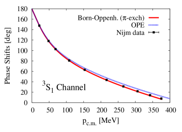
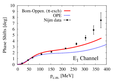
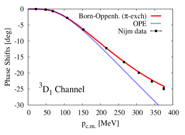
Figure 1: Renormalized (eigen) phase shifts for the OPE and $\Delta$-Born-Oppenheimer potentials as a function of the CM np momentum $p$ in the spin singlet ${}^{1}S_{0}$ (one counterterm) and triplet ${}^{3}S_{1}-^{3}D_{1}$ (three counterterms) channels compared to averaged Nijmegen potentials [17]. We take $f_{\pi NN}^{2}/4\pi=0.07388$[17] and $f_{\pi N\Delta}/f_{\pi NN}=6\sqrt{2}/5$.

Actually, Eq. (22) was evaluated in the Skyrme soliton model within the Heitler-London approximation, i.e. the product ansatz in the coupled channel space [36, 37] providing the long sought mid range attraction [12].  We reproduce the same results in the quark model calculation. The potential found using Feynman graph techniques [39] looks very similar with identical short distance singular behaviour identifying $h_{A}/g_{A}=f_{\pi N\Delta}/2f_{\pi NN}$. Note that we leave out background $\pi N$ scattering which correspond to triangle and box TPE diagrams at the quark level. The renormalization procedure as well as the necessary counterterms in the general coupled channel singular potentials has been explained in much detail in Ref. [32, 40]. The results for the phase shifts using Eq. (22) in the lowest partial waves are depicted in Fig. 1. In any case the description looks extremely similar (including deuteron properties) to the renormalization [41] of more sophisticated field theoretical potentials [39]. Convergence is achieved already at $r_{c}\sim 0.5{\rm fm}$.

The multiplicative structures of Eq. (22) reflect spin-flavour excitations and remind of the analogous Van der Waals forces in atomic systems. They hold literally even after inclusion of form factors with folded potentials (although $\Lambda_{\pi NN}$, $\Lambda_{\pi N\Delta}$ and $\Lambda_{\pi\Delta\Delta}$ are not necessarily identical) which remove the singularity. This is not equivalent to regularize the effective potential as a whole through subtractions. We have checked that form factors after renormalization become marginal in agreement with the OBE analysis [9].

7 Wigner SU(4) as a long distance symmetry

If the tensor force component of the qq potential, Eq. (7), is neglected one has invariance under the spin-isospin $SU(4)$ group with the quarks in the fundamental ${\bf 4}$-dimensional representation, $q=(u\uparrow,u\downarrow,d\uparrow,d\downarrow)$. In the three quark system we have the spin-flavour states ${\bf 4}\otimes{\bf 4}\otimes{\bf 4}={\bf 4}_{A}\oplus{\bf 20}_{S}\oplus{\bf 20}_{M_{1}}\oplus{\bf 20}_{M_{2}}$. Due to colour antisymmetry only the symmetric state survives which spin-isospin, $(S,T)$, decomposition is ${\bf 20}_{S}=(\frac{1}{2},\frac{1}{2})\oplus(\frac{3}{2},\frac{3}{2})=N\oplus\Delta$ yielding $N-\Delta$ degeneracy. Since $M_{\Delta}-M_{N}$ is large at nuclear scales, one might still treat the Nucleon quartet $N=(p\uparrow,p\downarrow,n\uparrow,n\downarrow)$ as the fundamental rep. of the old Wigner-Hund $SU(4)$ symmetry which implies spin independence, in particular that $V_{{}^{1}S_{0}}(r)=V_{{}^{3}S_{1}}(r)$ at all distances suggesting that phases $\delta_{{}^{1}S_{0}}(p)=\delta_{{}^{3}S_{1}}(p)$ in contradiction to data (see e.g. Fig. 1). The amazing finding of Ref. [6] was that assuming identical potentials $V_{{}^{1}S_{0}}(r)=V_{{}^{3}S_{1}}(r)$ for $r>r_{c}\to 0$ one has

$$p\cot\delta_{{}^{1}S_{0}}(p)=\frac{\alpha_{{}^{1}S_{0}}{\cal A}(p)+{\cal B}(p)}{\alpha_{{}^{1}S_{0}}{\cal C}(p)+{\cal D}(p)}\,,\qquad p\cot\delta_{{}^{3}S_{1}}(p)=\frac{\alpha_{{}^{3}S_{1}}{\cal A}(p)+{\cal B}(p)}{\alpha_{{}^{3}S_{1}}{\cal C}(p)+{\cal D}(p)}\,,$$ (23)

where the functions ${\cal A}(p)$, ${\cal B}(p)$, ${\cal C}(p)$ and ${\cal D}(p)$ are identical in both channels, but the experimentally different scattering lengths $\alpha_{{}^{1}S_{0}}=-23.74{\rm fm}$ and $\alpha_{{}^{3}S_{1}}=5.42{\rm fm}$ yield quite different phase shifts with a fairly good agreement. Thus, Wigner symmetry is broken by very short distance effects and hence corresponds to a long distance symmetry (a symmetry broken only by counterterms). Moreover, large $N_{c}$ [23] suggests that Wigner symmetry holds only for even L, a fact verified by phase shift sum rules [6]. In Refs. [7, 8] we analyze further the relation to the old Serber symmetry which follows from vanishing P-waves in $S=1$ channels, showing how old nuclear symmetries are unveiled by coarse graining the NN interaction via the $V_{\rm lowk}$ framework [42] and with testable implications for Skyrme forces in mean field calculations [43].

The chiral quark model is supposedly an approximate non-perturbative description, but perturbative gluons may be introduced by standard minimal coupling [13], $i\hbox to0.0pt{\hbox to5.30904pt{\hfil/\hfil}\hss}\partial\to i\hbox to0.0pt{\hbox to5.30904pt{\hfil/\hfil}\hss}\partial+g\hbox to0.0pt{\hbox to7.50002pt{\hfil/\hfil}\hss}A^{a}\cdot{\lambda^{c}_{a}}/2$ with $\lambda^{c}_{a}$ the $N_{c}^{2}-1$ Gell-Mann colour matrices. A source of $SU(4)$ breaking is the contact one gluon exchange which yields spin-colour chromo-magnetic interactions ($S_{ij}$ is the tensor operator),

$$V^{\rm OGE}=\frac{1}{4}\alpha_{s}\sum_{i<j}(\lambda_{i}^{c}\cdot\lambda_{j}^{c})\left\{\frac{1}{r_{ij}}-\frac{\pi}{4m_{i}m_{j}}\left[1+\frac{2}{3}\sigma_{i}\cdot\sigma_{j}\right]\delta^{(3)}(\vec{r}_{ij})-\frac{3}{4m_{i}m_{j}r_{ij}}S_{ij}\right\}$$ (24)

breaking the $\Delta-N$ degeneracy. This short distance terms break also the ${}^{1}S_{0}$ and ${}^{3}S_{1}$ degeneracy of the $NN$ system providing an understanding of the long distance character of Wigner symmetry. Taking the Wigner symmetric zero energy state and perturbing around it, the previous argument suggests that $1/\alpha_{{}^{3}S_{1}}-1/\alpha_{{}^{1}S_{0}}={\cal O}(M_{\Delta}-M_{N})$ with a computable coefficient.

8 Conclusions

Chiral Quark and Soliton models while quite different in appearance provide some universal behaviour regarding $NN$ interactions. If the asymptotic potentials coincide, the main differences in describing the scattering data are due to a few low energy constants which in some cases are subjected to extreme fine tuning of the model parameters. The success of the model at finite energy is mainly reduced to reproducing these low energy parameters.

One of us (E.R.A.) warmly thanks M. Rosina, B. Golli and S. Širca for the invitation and D. R. Entem, F. Fernandez, M. Pavón Valderrama and J. L. Goity for discussions. This work is supported by the Spanish DGI and FEDER funds with grant FIS2008-01143/FIS, Junta de Andalucía grant FQM225-05, and EU Integrated Infrastructure Initiative Hadron Physics Project contract RII3-CT-2004-506078.

References

- [1] R. Machleidt, K. Holinde and C. Elster, Phys. Rept. 149 (1987) 1.
- [2] M.M. Nagels, T.A. Rijken and J.J. de Swart, Phys. Rev. D17 (1978) 768.
- [3] M. Pavon Valderrama and E. Ruiz Arriola, Phys. Rev. C72 (2005) 054002.
- [4] E. Ruiz Arriola, A. Calle Cordon and M. Pavon Valderrama, (2007), 0710.2770.
- [5] A. Calle Cordon and E. Ruiz Arriola, AIP Conf. Proc. 1030 (2008) 334.
- [6] A. Calle Cordon and E. Ruiz Arriola, Phys. Rev. C78 (2008) 054002.
- [7] A. Calle Cordon and E. Ruiz Arriola, Phys. Rev. C80 (2009) 014002.
- [8] E. Ruiz Arriola and A. Calle Cordon, (2009), 0904.4132.
- [9] A. Calle Cordon and E. Ruiz Arriola, (2009), 0905.4933.
- [10] M. Oka and K. Yazaki, Int. Rev. Nucl. Phys. 1 (1984) 489.
- [11] R.F. Alvarez-Estrada, F. Fernandez, J. L. Sanchez-Gomez and V. Vento, Lect. Notes Phys. 259 (1986) 1.
- [12] T.S. Walhout and J. Wambach, Int. J. Mod. Phys. E1 (1992) 665.
- [13] A. Valcarce, H. Garzilazo, F. Fernandez and P. Gonzalez, Rept. Prog. Phys. 68 (2005) 965.
- [14] N. Ishii, S. Aoki and T. Hatsuda, Phys. Rev. Lett. 99 (2007) 022001.
- [15] S. Aoki, T. Hatsuda and N. Ishii, (2009), 0909.5585.
- [16] H.B. O’Connell et al., Prog. Part. Nucl. Phys. 39 (1997) 201.
- [17] V.G.J. Stoks et al., Phys. Rev. C49 (1994) 2950.
- [18] M.B. Gavela et al., Phys. Lett. B82 (1979) 431.
- [19] O.W. Greenberg and H.J. Lipkin, Nucl. Phys. A370 (1981) 349.
- [20] C.V. Christov et al., Prog. Part. Nucl. Phys. 37 (1996) 91.
- [21] H. Weigel, Lect. Notes Phys. 743 (2008) 1.
- [22] E. Ruiz Arriola, W. Broniowski and B. Golli, Phys. Rev. D76 (2007) 014008.
- [23] D.B. Kaplan and A.V. Manohar, Phys. Rev. C56 (1997) 76.
- [24] M.C. Birse and M.K. Banerjee, Phys. Lett. B136 (1984) 284.
- [25] A. Manohar and H. Georgi, Nucl. Phys. B234 (1984) 189.
- [26] L.Y. Glozman and D.O. Riska, Phys. Rept. 268 (1996) 263.
- [27] J.L. Goity, Phys. Atom. Nucl. 68 (2005) 624.
- [28] D. Bartz and F. Stancu, Phys. Rev. C63 (2001) 034001.
- [29] D. R. Entem, E. Ruiz Arriola, M. Pavon Valderrama and R. Machleidt, Phys. Rev. C77 (2008) 044006.
- [30] M.T. Fernandez-Carames, P. Gonzalez and A. Valcarce, Phys. Rev. C77 (2008) 054003.
- [31] G. Karl and J.E. Paton, Phys. Rev. D30 (1984) 238.
- [32] M. Pavon Valderrama and E. Ruiz Arriola, Phys. Rev. C74 (2006) 054001.
- [33] A.M. Green, Rept. Prog. Phys. 39 (1976) 1109.
- [34] G.H. Niephaus, M. Gari and B. Sommer, Phys. Rev. C20 (1979) 1096.
- [35] R.B. Wiringa, R.A. Smith and T.L. Ainsworth, Phys. Rev. C29 (1984) 1207.
- [36] N.R. Walet, R.D. Amado and A. Hosaka, Phys. Rev. Lett. 68 (1992) 3849.
- [37] N.R. Walet and R.D. Amado, Phys. Rev. C47 (1993) 498.
- [38] G. Holzwarth and R. Machleidt, Phys. Rev. C55 (1997) 1088.
- [39] N. Kaiser, S. Gerstendorfer and W. Weise, Nucl. Phys. A637 (1998) 395.
- [40] M. Pavon Valderrama and E. Ruiz Arriola, Annals Phys. 323 (2008) 1037.
- [41] M. Pavon Valderrama and E. Ruiz Arriola, Phys. Rev. C79 (2009) 044001.
- [42] S. K. Bogner, T. T. S. Kuo and A. Schwenk, Phys. Rept. 386 (2003) 1
- [43] M. Zalewski, J. Dobaczewski, W. Satula and T. R. Werner, Phys. Rev. C77 (2008) 024316