Large-Scale CO Maps of the Lupus Molecular Cloud Complex

Abstract

Fully sampled degree-scale maps of the ¹³CO 2–1 and CO 4–3 transitions toward three members of the Lupus Molecular Cloud Complex — Lupus I, III, and IV — trace the column density and temperature of the molecular gas. Comparison with IR extinction maps from the c2d project requires most of the gas to have a temperature of 8–10 K. Estimates of the cloud mass from ¹³CO emission are roughly consistent with most previous estimates, while the line widths are higher, around 2 km s^-1. CO 4–3 emission is found throughout Lupus I, indicating widespread dense gas, and toward Lupus III and IV. Enhanced line widths at the NW end and along the edge of the B 228 ridge in Lupus I, and a coherent velocity gradient across the ridge, are consistent with interaction between the molecular cloud and an expanding H I shell from the Upper-Scorpius subgroup of the Sco-Cen OB Association. Lupus III is dominated by the effects of two HAe/Be stars, and shows no sign of external influence. Slightly warmer gas around the core of Lupus IV and a low line width suggest heating by the Upper-Centaurus-Lupus subgroup of Sco-Cen, without the effects of an H I shell.

1 Introduction

The Lupus star forming region, recently reviewed by Comerón (2008), lies about 150 pc from the Earth (Lombardi et al., 2008a), in the Gould Belt. It is immediately visible by inspection of optical photographs of the sky, comprising a set of largely filamentary dark clouds. Based on optical extinction maps (Cambrésy, 1997), the ‘Cores to Disks’ Spitzer Legacy Programme (c2d, Evans et al., 2003, 2007, 2009), has produced and analyzed infrared images of three areas: Lupus I, III, and IV. The c2d data products (Evans et al., 2007) include: shorter-wavelength Infrared Array Camera (IRAC) maps, used to identify and classify young stellar objects (YSOs, Merín et al., 2008); far-IR MIPS maps (Chapman et al., 2007) tracing the thermal emission of the dust component of the molecular clouds; and IR extinction maps, based on the Two Micron All Sky Survey (2MASS; Chapman et al., 2007) and on a combination of 2MASS and IRAC data (Evans et al., 2007). In this paper, we present maps of the c2d fields in Lupus, tracing the molecular hydrogen by the rotational emission of carbon monoxide (CO) and isotopically substituted ¹³CO.

The Lupus complex has been extensively surveyed in the various 1–0 transitions of CO: Murphy et al. (1986) first mapped the Lupus molecular clouds using the 1.2 m Columbia telescope with 0.5° resolution to show the extent of the molecular gas in Lupus and suggest a total mass of a few $10^{4}$ $M_{\sun}$. Improved maps in several transitions were obtained by NANTEN (2.7′ resolution, but routinely undersampled): Tachihara et al. (2001) published ¹²CO maps of the whole complex, mostly sampled at 8′ spacing, with some areas at 4′ spacing; ¹³CO 1–0 maps (Tachihara et al., 1996) cover Lupus I and III with 8′ spacing, while C¹⁸O 1–0 maps (Hara et al., 1999) cover all the clouds in the complex at 2′ spacing. Moreira & Yun (2002) mapped about 200 arcmin² of Lupus IV at sub-arcminute resolution and full-beam spacing in the 1–0 transitions of CO, ¹³CO, and C¹⁸O. The ¹³CO 2–1 and CO 4–3 maps presented here are the first large-scale fully sampled low-$J$ CO maps of Lupus, and the first mid-$J$ CO maps of any kind.

The large-scale structure of the Lupus clouds can be traced by near-IR extinction (Lombardi et al., 2008b) and CO 1–0 emission (Tachihara et al., 2001). The complex covers some 20° of galactic latitude (about 50 pc). At low latitudes ($b\lesssim 10^{\circ}$), a large mass of diffuse gas contains denser filamentary clouds; at higher latitudes, the dense clouds (Lupus I and II) are more clearly separated. The evolution of the Lupus clouds may have been driven by the influence of nearby OB stars (Tachihara et al., 2001). The Lupus and Ophiuchus molecular clouds face one another across the Upper-Scorpius subgroup of the Scorpius-Centaurus OB Association; the Upper-Centaurus-Lupus subgroup lies on the opposite side of the Lupus clouds from Upper-Sco. The H I shell around Upper-Sco, blown by stellar winds and a presumed supernova 1.5 Myr ago (de Geus, 1992), borders the NE side of the Lupus clouds; on the plane of the sky, the ridge which dominates Lupus I (B 228, see below) lies just on the trailing edge of the H I shell. The much older Upper-Cen-Lup subgroup has driven an H I shell far beyond the Lupus clouds (de Geus, 1992); it should have passed through the Lupus complex some 4–7 Myr ago, roughly consistent with the ages of T Tauri stars in Lupus III and IV (Moreira & Yun, 2002).

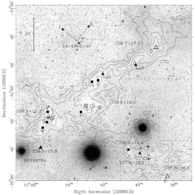
Figure 1: Optical (blue DSS2) image of Lupus I, overlaid with ¹³CO 2–1 emission from this work (contours at 1, 3, 5, 7, 9 K km s^-1). Annotations: dark cloud positions (Table 1) from Hartley et al. (1986, open triangles), Vilas-Boas et al. (2000, filled triangles), and Lee & Myers (1999, squares); embedded YSOs from Merín et al. (2008, star-shapes); bright stars (by name); C¹⁸O 1–0 peaks from Hara et al. (1999, diamonds). Filled squares denote cloud cores observed in molecular lines by Lee et al. (2004). Only objects within the ¹³CO map are plotted. The $l,b$ arrows are 15′ long.

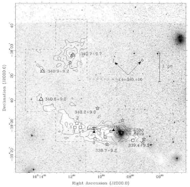
Figure 2: Optical image of Lupus III, as in Figure 1. ¹³CO contours are at 2, 4, …12 K km s^-1. Bright stars are marked as crosses.

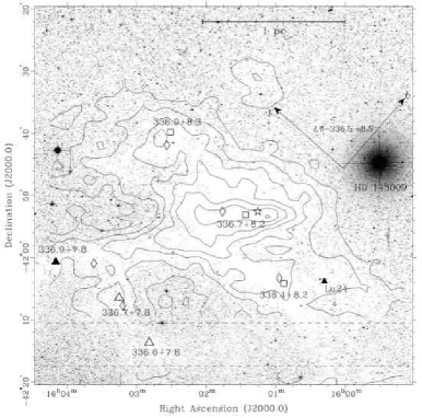
Figure 3: Optical image of Lupus IV, as in Figure 1. ¹³CO contours are at 1, 2, …7 K km s^-1.

Lupus I (Figure 1) is dominated by B 228 (Barnard, 1927) or GF 19 (Schneider & Elmegreen, 1979), a long ridge running NW–SE, extending over about 2° (5 pc) parallel to the edge of the Upper-Sco H I shell. The molecular material appears to fall off steeply toward the center of the shell (at the NE edge), but there is extensive material on the other side of the ridge. Lupus III (Figure 2) is a long (about $4\times 1$ pc) E–W cloud (GF 21, Schneider & Elmegreen, 1979) at the edge of the low-latitude cloud mass: at its eastern end, it curves up to the NE and breaks up into clumps; toward the west lie two embedded (but optically visible) Herbig Ae/Be stars, HR 5999 (A 5–7) and the B 6 HR 6000 (Comerón, 2008). Tachihara et al. (2002) consider Lupus III to be a cluster-forming structure with a dense head and spread-out tail, analogous to the $\rho$ Oph and Cha I clouds. A couple of pc north of Lupus III, there is another smaller cloud, which appears to be a separate condensation in the low-latitude gas; we henceforth refer to this northern structure as Lupus III N. Lupus IV (Figure 3) is the head of a filamentary structure running approximately E–W (GF 17, Schneider & Elmegreen, 1979; Moreira & Yun, 2002), comprising a small core, about 0.5 pc long (E–W), lying within a more diffuse extended cloud, about a pc across. The filament connects Lupus IV to the low-latitude gas mass to the East; Schneider & Elmegreen describe it as a “chain of small faint globules”.

Individual dark clouds or cloud peaks have been identified by inspection of optical surveys on scales ranging from degrees (e.g., B 228) to arcminutes (Sandqvist & Lindroos, 1976; Feitzinger & Stüwe, 1984; Hartley et al., 1986; Bourke et al., 1995a; Andreazza & Vilas-Boas, 1996; Lee & Myers, 1999; Vilas-Boas et al., 2000); these clouds are listed in Table 1. Near-IR extinction maps of Lupus III with a resolution of 30″ (Teixeira et al., 2005) have been used to identify dark cores in more detail, which were then fitted with Bonnor-Ebert profiles. Single-pointing spectra in several molecular lines have been observed toward extinction-selected clumps: Sandqvist & Lindroos (1976) observed H₂CO along four lines of sight at 6 cm (6.6′ beamwidth); Bourke et al. (1995b) searched for ammonia, but did not detect it, toward two globules (BHR 120 & 140); Vilas-Boas et al. (2000) observed ¹³CO and C¹⁸O 1–0, but their 0.8′ beamwidth is poorly-matched to ours; Lee et al. (2004) observed a few of their Lupus I cores (Lee & Myers, 1999) in CS 3–2 and DCO⁺ 2–1 (0.7′ beamwidth). Previously identified CO cores, both those observed by Vilas-Boas et al., and those identified from their C¹⁸O maps by Hara et al. (1999), are listed in Table 2. The positions of these extinction cores and C¹⁸O cores with respect to optical and ¹³CO 2–1 emission are shown in Figures 1–3. Of the members of the c2d small dark cloud sample mapped by AST/RO in ¹³CO 2–1 and CO 4–3 (Löhr et al., 2007), three lie within the Lupus region, but outside our maps.

Lupus I contains a few YSOs, concentrated to the B 228 ridge (Merín et al., 2008). Lupus III contains a very dense cluster of YSOs near the Herbig Ae/Be stars, composed mainly of T Tauri stars (Allen et al., 2007; Merín et al., 2008), but including the Class 0 object Lupus 3 MMS (Tachihara et al., 2007). Comerón et al. (2009) identified a population of cool stars and brown dwarfs toward Lupus I and III, which are not strongly concentrated toward the molecular clouds. The Lupus IV region contains about as many YSOs as the Lupus I region (Merín et al., 2008), but they are older (Class II/III) and largely found outside the molecular cloud, with the exception of one flat-spectrum YSO candidate close to the cloud center. Even the dispersed population is absent (Comerón et al., 2009). Lupus IV thus appears to have less (or no) ongoing star formation, compared to Lupus I and III. Merín et al. suggest that the Class II and III YSOs surrounding it represent an earlier generation of star formation (possibly associated with the passage of the Upper-Cen-Lup H I shell mentioned above), and that the very dense Lupus IV core is poised to form new stars. The younger YSOs (Class 0, I, and flat-spectrum sources from the c2d samples, Merín et al., 2008) within the boundaries of our ¹³CO 2–1 maps are listed in Table 3, and plotted in Figures 1–3.

2 Observations

Lupus I, III, and IV were observed with the Antarctic Submillimeter Telescope and Remote Observatory (AST/RO, Stark et al., 2001), during the period 2005 March–November, in the 461 GHz CO 4–3 and 220 GHz ¹³CO 2–1 transitions. The telescope, receiver, and spectrometer systems are described by Stark et al. (2001): ¹³CO 2–1 observations used the 230 GHz SIS receiver, whose local oscillator system has been upgraded to use a synthesizer, frequency multiplied ($\times 19$) by a Millitech multiplier. CO 4–3 observations used the 450–495 GHz SIS waveguide receiver (Walker et al., 1992). Low-resolution acousto-optical spectrometers (AOSs, 1 GHz bandwidth, 0.7 MHz channel width) were used for all observations.

The large-scale maps presented in this paper were built up from multiple smaller maps (‘submaps’), mosaicked together as follows: each submap was centered on a point of a large-scale grid superimposed on the molecular cloud, the grid points separated by 24′ and 12′ for the 2–1 and 4–3 observations respectively. The submaps measure $28\arcmin\times 29\arcmin$ ($\alpha\times\delta$) and $12\arcmin\times 12\arcmin$ respectively, giving substantial overlap between neighbouring 2–1 maps and some overlap (one row or column of spectra) between neighbouring 4–3 maps.

The submaps use cell sizes of 1′ and 0.5′, significantly oversampling the telescope beam (3.3′ at 220 GHz, 1.7′ at 461 GHz). The spectra are position switched, taken in batches of 4 or 5, all of which share a reference measurement, about a degree away. The 4 or 5 source spectra are all at the same declination (and hence at the same elevation, since AST/RO lies at the South Geographic Pole), but the reference position is the same for all spectra in a submap, and may thus differ in elevation from the source spectra by as much as a few arcminutes. The use of one reference position for each submap, however, allows the reference position to be checked for emission. Each row of each submap is built up from a number of contiguous blocks of reference-sharing spectra. Reference sharing increases the observing efficiency almost to that of on-the-fly mapping, but also shares one of its weaknesses: the sharing of a reference spectrum produces correlated noise in neighboring spectra, which can show up as artifacts in the map. Rather than the long stripes characteristic of on-the-fly mapping, correlated noise is manifested in the AST/RO maps as short (4- or 5-cell) horizontal blocks.

3 Data Reduction

The AST/RO observing system produces spectra calibrated onto the $T^{*}_{A}$ scale (Stark et al., 2001); because of the unobstructed off-axis optical design of the telescope, this is essentially equivalent to $T^{*}_{R}$. Further reduction and processing were carried out (using COMB, the standard AST/RO data reduction program, and PDL). The spectra have velocity resolutions of 0.9 km s^-1 (¹³CO 2–1) and 0.4 km s^-1 (CO 4–3); they were checked for frequency shifts, and corrections were applied (corrections ranged from 0 to almost 5 km s^-1 — see Appendix A). Linear baselines were subtracted from all spectra, along with polynomial baselines if necessary: a few percent of the 4–3 spectra required non-linear baseline subtraction, and almost none of the 2–1 spectra (Table 4).

Long-integration spectra were taken toward all reference positions, generally showing upper limits of $\sim 0.1$ K (¹³CO 2–1) and $\sim 0.3$ K (CO 4–3). Some 2–1 reference positions (for one submap in Lupus I and one in Lupus III) contained substantial emission ($\sim 1$ K), and these reference spectra were added back into all the spectra in the relevant submap.

Because of the overlap between submaps, there are over a thousand pointings on the sky toward which two or more spectra were measured at different times. These duplicate pointings can be used to estimate the internal consistency of the flux calibration at the telescope. Distributions of the ratios of peak $T^{*}_{R}$ between spectra with the same pointings are shown in Figure 4 for both 4–3 and 2–1 data. The typical inconsistencies between these spectra (estimated by the standard deviation of the distributions of $T^{*}_{R}$ ratios) are about 30% for CO 4–3 data, and about 20% for ¹³CO 2–1.

3.1 Map Making

Initial map making was carried out by nearest-neighbor sampling the submap data onto one large grid, with overlapping observations co-added. Each pixel of these maps corresponds directly to the spectrum observed by the telescope; without smoothing, inconsistencies between neighbouring submaps show up as clear edges, which are much more obvious in the 4–3 than in the 2–1 data.

The overlap between submaps allowed these inconsistencies in the 4–3 data to be checked and corrected. Individual submaps with significantly different flux scales to their surroundings were identified and rescaled. These rescalings were checked visually: a submap was only rescaled if it was obviously higher or lower than its neighbours, if the measured scaling was consistent with the visual one, and if the rescaling improved the appearance of the map when it was applied. Rescaling corrections of $\lesssim 10$% did not significantly improve the appearance of the map, and were not implemented. Fewer than half the submaps needed correction, mostly by factors of 0.7–1.4 (in line with the estimate of internal consistency given above), and the largest correction factor was $\sim 1.8$. No corrections needed to be applied to the 2–1 data. The need to rescale probably arises from imperfect estimation of the atmospheric transparency in the calibration procedure, which works better when the atmosphere is fairly optically thin (e.g. at 220 GHz) than at higher opacities (e.g., at 461 GHz).

The corrected 4–3 data (and uncorrected 2–1 data) were then gridded (as above) to produce final unsmoothed data cubes, which were used to generate the maps in this paper. All the quantities mapped are calculated directly from the data, without profile-fitting. For example, the line width is estimated by the ratio of integrated intensity to peak $T^{*}_{R}$ (which overestimates the FWHM by about 10% if applied to a perfect gaussian line). Sample spectra from the data cubes are shown in Figures 5–7.

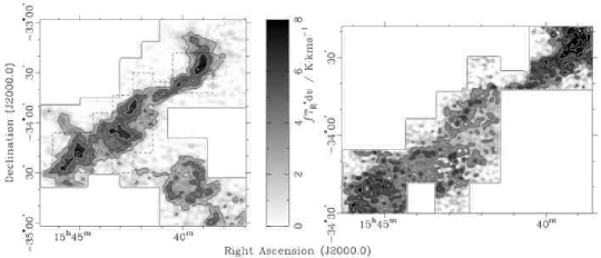
Figure 8: Maps of Lupus I in (left) ¹³CO 2–1 and (right) CO 4–3, integrated from $v_{LSR}=+2$ to $+10$ km s^-1. ¹³CO 2–1 contours at 2, 4 K km s^-1 (black) and 6, 8 K km s^-1 (white); CO 4–3 contours at 3, 5 (black) and 7, 9, 11 K km s^-1 (white). The broken outline denotes the extent of the CO 4–3 map.

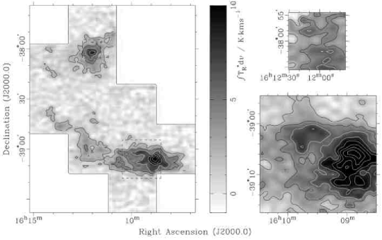
Figure 9: Maps of Lupus III and Lupus III N in (left) ¹³CO 2–1, integrated from $v_{LSR}=+2$ to $+12$ km s^-1, and (right) CO 4–3, integrated from $v_{LSR}=+2$ to $+8$ km s^-1 toward Lupus III and from $+6$ to $+12$ km s^-1 toward Lupus III N. Contours at 2, 4 K km s^-1 (black) and 6, 8…16 K km s^-1 (white).

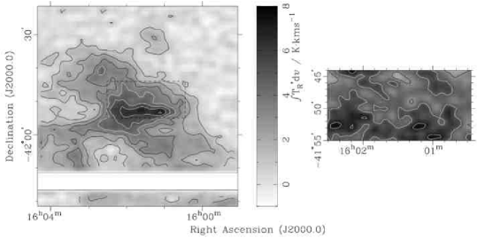
Figure 10: Maps of Lupus IV in (left) ¹³CO 2–1 and (right) CO 4–3, integrated from $v_{LSR}=+3$ to $+7$ km s^-1. ¹³CO 2–1 contours at 1, 2, 3 K km s^-1 (black) and 4, 5, 6, 7 K km s^-1 (white); CO 4–3 contours at 3 K km s^-1 (black) and 5, 7 K km s^-1 (white).

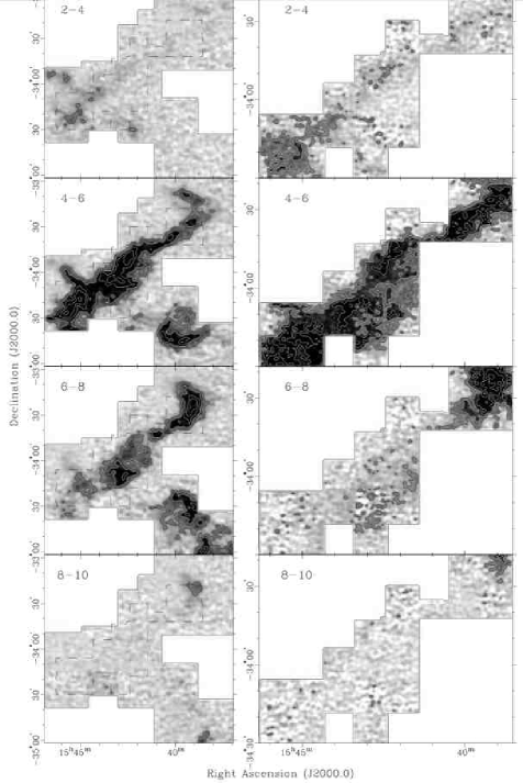
Figure 11: Channel maps of Lupus I in (left) ¹³CO 2–1 and (right) CO 4–3, labeled with $v_{LSR}$ range in km s^-1. Contours at 1 K km s^-1 (black) and 2, 3,…6 K km s^-1 (white). Broken outlines denote the extent of the CO 4–3 map.

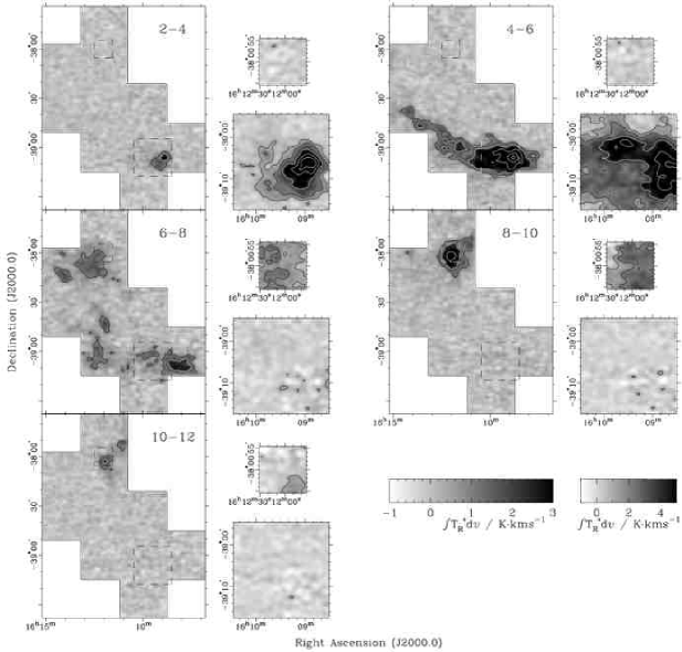
Figure 12: Channel maps of Lupus III, as in Figure 11. ¹³CO 2–1 contours are at 1 K km s^-1 (black) and 2, 4, 6, 8 K km s^-1 (white); CO 4–3 contours are at 1, 2 K km s^-1 (black) and 4, 6, 8 K km s^-1 (white).

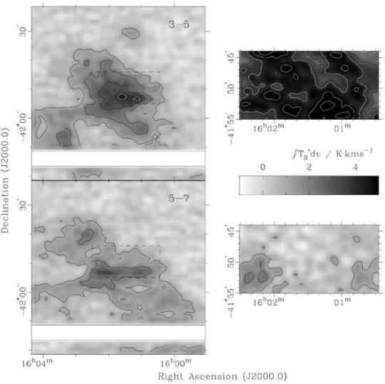
Figure 13: Channel maps of Lupus IV, as in Figure 11. Contours at 1, 2, 3 K km s^-1 (black) and 4, 5, 6 K km s^-1 (white).

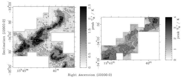
Figure 14: Maps of the peak $T_{R}^{*}$ of (left) ¹³CO 2–1 and (right) CO 4–3 toward Lupus I. Left: contours at 0.5, 1 K (black) and 1.5, 2.5, 3.5 K (white). Right: contours at 1.5, 2 K (black) and 2.5, 3, 3.5, 4 K (white). The broken outline denotes the extent of the CO 4–3 map.

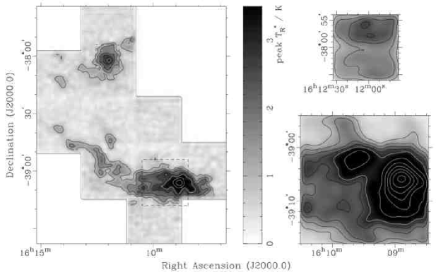
Figure 15: Maps of the peak $T_{R}^{*}$ toward Lupus III, as in Figure 14: contours at 1, 1.5, 2, 2.5 K (black) and 3, 4,…9 K (white).

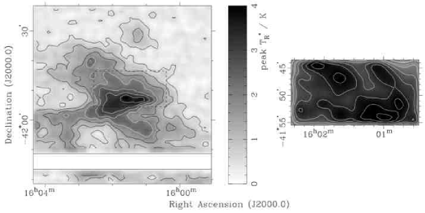
Figure 16: Maps of the peak $T_{R}^{*}$ toward Lupus IV, as in Figure 14: contours at 0.5, 1, 1.5 K (black) and 2, 2.5,…4.5 K (white).

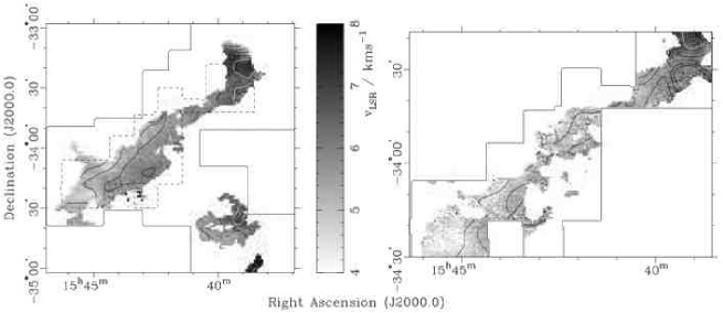
Figure 17: Maps of the centroid velocity of (left) ¹³CO 2–1 and (right) CO 4–3 emission toward Lupus I. Contours are at 5, 5.5, 6 km s^-1 (black) and 6.5, 7, 7.5 km s^-1 (white). The gray scale is unsmoothed, while the contours have been smoothed with a Gaussian kernel. Only spectra with S/N$>$10 are shown. Solid outlines indicate the extent of the maps, while the broken outline indicates the extent of the CO 4–3 map.

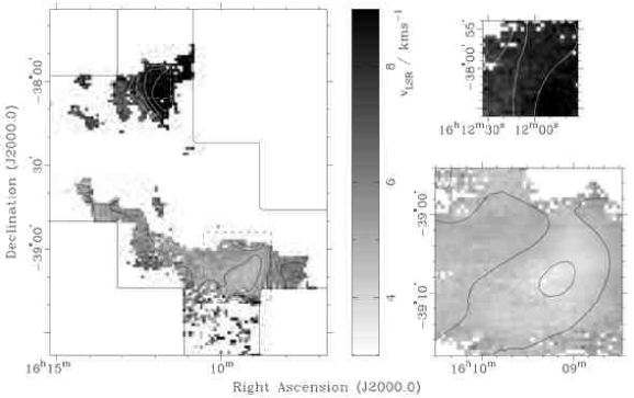
Figure 18: Maps of the centroid velocity of emission toward Lupus III, as in Figure 17: ¹³CO 2–1 contours are at 5, 5.5, 6 km s^-1 (black) and 7.5, 8, 8.5, 9 km s^-1 (white); CO 4–3 contours are at 4, 4.5,km s^-1 (black) and 7.5, 8, 8.5, 9 km s^-1 (white). Only spectra with S/N$>$5 are shown.

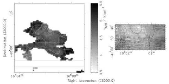
Figure 19: Maps of the centroid velocity of emission toward Lupus IV, as in Figure 17: contours are at 4, 4.3 (black) and 4.6, 4.9, 5.2 km s^-1 (white). Only spectra with S/N$>$10 are shown.

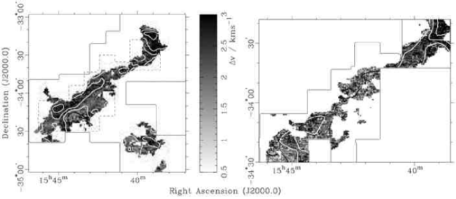
Figure 20: Maps of the line widths of (left) ¹³CO 2–1 and (right) CO 4–3 toward Lupus I. Contours are at 2, 2.4,…3.6 km s^-1. Gray scale is unsmoothed, while contours have been smoothed with a Gaussian kernel. Only spectra with S/N$>$10 are shown. Solid outlines indicate the extent of the maps, while the broken outline indicates the extent of the CO 4–3 map.

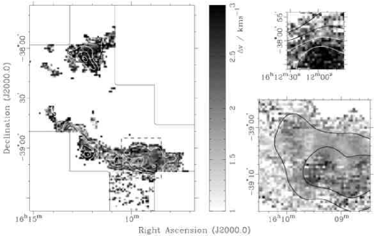
Figure 21: Maps of emission line widths toward Lupus III, as in Figure 20: contours are at 1.5, 1.8, 2.1 km s^-1 (black) and 2.4, 2.7, 3 km s^-1 (white). Only spectra with S/N$>$5 are shown.

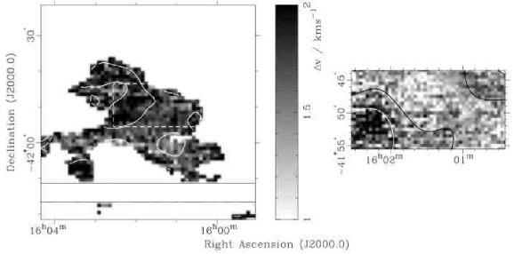
Figure 22: Maps of emission line widths toward Lupus IV, as in Figure 20: contours at 1.4, 1.6 km s^-1 (black) and 1.8, 2 km s^-1 (white). Only spectra with S/N$>$10 are shown.

Integrated intensity maps (Figures 8–10), channel maps (integrated over 2 km s^-1 channels, Figures 11–13), and peak $T^{*}_{R}$ maps (Figures 14–16) were all produced by bessel smoothing (e.g. Jenness & Lightfoot, 2000), which gives the ‘most fair’ representation of the sky as observed by a single-dish telescope. However, if significant emission extends to the edge of the map, this technique tends to produce a roll-off of emission in the outermost pixels of the map, and this effect is visible in some of the Lupus maps. The effective telescope diameter was picked to balance resolution against noise: 1.5 m for the 2–1 maps, and 1.2 m for the 4–3, yielding overall beam sizes of 3.8′ and 2.3′, respectively. Maps of the velocity centroid (Figures 17–19) and line width (Figures 20–22) use both unsmoothed data (in grayscale) and Gaussian-smoothed data (contours), with Gaussian FWHMs of 5′ (2–1) and 5.75′ (4–3) yielding overall beams of 6′ in both transitions.

The nominal pointing accuracy of AST/RO is about 1′, but comparison of the ¹³CO 2–1 map of Lupus IV with the optical extinction structure (see Figure 3) suggests a systematic offset in declination. Discrepancies of similar magnitude can be seen in other AST/RO data from 2005 (Löhr et al., 2007). The Lupus IV maps have therefore all been shifted southwards by 1.5′. The submillimeter map is well correlated with the millimeter-wave one, and so it has been shifted as well. There is no evidence of similar systematic shifts in the Lupus I or Lupus III data. The publicly available data cubes do not have this shift applied to them.

4 Results

4.1 Overview of the Lupus Clouds

Vilas-Boas et al. (2000) estimated C¹⁸O 1–0 optical depths in the range 0.1–0.5 toward extinction peaks, implying that ¹³CO 2–1 will no longer be optically thin in dense parts of the Lupus clouds. Maps of ¹³CO 2–1 peak $T^{*}_{R}$ follow the extinction maps of Chapman et al. (2007) better than maps of integrated intensity do, suggesting widespread breakdown of the optically thin approximation. The maximum peak $T^{*}_{R}$ toward Lupus I and IV is about 3.5 K in each map, implying a minimum excitation temperature, $T_{x}$, of 8 K; the peak $T^{*}_{R}$ in Lupus III reaches 5 K near the bright stars, so $T_{x}\gtrsim 10$ K in this area. Tachihara et al. (1996) adopted 13 K for their analysis of ¹³CO 1–0 toward Lupus I. A comparison of the lower ¹³CO contours to the most recent c2d extinction maps suggests that excitation temperatures of 8–10 K will reproduce the extinction-traced column density quite well. While higher excitation temperatures are not ruled out by the molecular line data, they would lead to lower column density estimates which would be less compatible with estimates from extinction, which is probably the least biased estimator of the true column density (Goodman et al., 2009).

Gas masses are estimated from the ¹³CO 2–1 data as follows: the ratio of the peak $T^{*}_{R}$ to the maximum possible brightness temperature (for assumed $T_{x}$) yields an estimate of the peak optical depth $\tau_{0}^{(13)}$; this is multiplied by the line width to estimate $\int\tau dv$, which is proportional to the column density of ¹³CO ($N^{(13)}$, Appendix B). $N^{(13)}$ is converted to a total gas column density by assuming conversions between $N^{(13)}$ and extinction $A_{V}$ (see below), and between $A_{V}$ and the column density of hydrogen ($N_{\rm H}=1.37\times 10^{21}A_{V}$ $\mathrm{cm^{-2}}$, Evans et al., 2009). Assuming a distance of 150 pc, the total gas mass enclosed in a 1 arcmin² pixel is then calculated.

The relationship between ¹³CO column density and extinction can be expressed as $N^{(13)}=x^{(13)}\times 10^{15}(A_{V}-A_{V,0})$ cm^-2, with the extinction threshold $A_{V,0}$ reflecting the minimum column density required for the presence of ¹³CO. The most commonly used parameters come from a study of $\rho$ Oph by Frerking et al. (1982, FLW): $x^{(13)}=2.7$ $\mathrm{cm^{-2}}$ $\mathrm{mag^{-1}}$, $A_{V,0}=1.6$ mag; other studies (e.g. Bachiller & Cernicharo, 1986; Lada et al., 1994) have found values of $x^{(13)}$ in the range 2.2–2.7, and extinction thresholds of 0–1.6 mag. Recently, a comprehensive study of the Perseus complex (Pineda et al., 2008) found $x^{(13)}=2.4$ $\mathrm{cm^{-2}}$ $\mathrm{mag^{-1}}$  $A_{V,0}=1.7$ mag overall, and $x^{(13)}=1.9$ $\mathrm{cm^{-2}}$ $\mathrm{mag^{-1}}$, $A_{V,0}=1.2$ mag toward the West End of the complex (PWE), comprising several dark clouds, which is likely to be the best analog to the Lupus clouds.

Estimated masses of the Lupus clouds above $A_{V}$ thresholds of 2 and 3 mag are given in Table 5, along with the mean and dispersion of the line widths of material with $A_{V}\geq 2$. (The line width distribution for $A_{V}\geq 3$ is very similar, varying only by about 0.1 km s^-1.) Masses have been calculated for $T_{x}=8,9,10$ K and for three ¹³CO-to-$A_{V}$ relations: PWE, Perseus, and FLW. The quoted mass is the estimate using $T_{x}=9$ K and PWE, and the positive and negative errors give the full range of mass estimates. Other estimates of mass and line width from the literature are also tabulated. Previous isotopically substituted CO results relied, directly or indirectly, on the older ratio of $N_{H}$ to $A_{V}$ ($1.87\times 10^{21}$ $\mathrm{cm^{-2}}$, Bohlin et al., 1978), and have been rescaled to use the same ratio as in this work. The extinction mass of Lupus III has also been rescaled to assume a distance of 150 pc instead of the 200 pc used by Chapman et al. (2007) and Evans et al. (2009).

The masses of Lupus I, III (including Lupus III N) and IV are estimated to be 280, 150, and 80 $M_{\odot}$ respectively (for $A_{V}\geq 2$). The extinction mass of Lupus I (251 $M_{\odot}$) is similar to the ¹³CO 2–1 estimate; those of Lupus III and IV are significantly greater (250 and 120 $M_{\odot}$), but still consistent with the ¹³CO 2–1 error range. This suggests that the Lupus complex has spatial variations in the ¹³CO-to-$A_{V}$ ratio, as Perseus does (Goodman et al., 2009). By contrast, the ¹³CO 1–0 mass estimate toward Lupus I is 880 $M_{\odot}$ (Tachihara et al., 1996). The ¹³CO 1–0 map covers a much larger area than ours (almost 10 deg²) and includes significant emission to the SE and SW of our map boundaries. Within the confines of the ¹³CO 2–1 map, we estimate that the ¹³CO 1–0 mass should be 600–700 $M_{\odot}$, still about 50% more than the upper limit of our mass range. A similar discrepancy was reported by Moreira & Yun (2002), whose mass estimate for Lupus II is about a factor of 3 lower than that of Tachihara et al.; but their mass estimate for Lupus IV is quite similar to ours. Possible reasons for the discrepancies include the undersampling of the NANTEN maps (which will tend to overestimate the area of structures) and differences in the calibration of the two telescopes. Hara et al. (1999) measured only 240 $M_{\odot}$ toward Lupus I in C¹⁸O 1–0, which is much closer to our estimate. The additional mass in the ¹³CO 1–0 map might comprise tenuous gas in which the 2–1 transition is not fully excited, and whose column density is low enough for it not to be detectable in C¹⁸O 1–0. The ¹³CO 1–0 mass estimate toward Lupus III (220 $M_{\odot}$) is consistent with our data and close to the extinction result, while the C¹⁸O 1–0 estimates toward Lupus III and III N (80 and 5 $M_{\odot}$) are much lower.

The average line widths for the Lupus clouds (Table 5 and Evans et al., 2009) have been deconvolved by subtracting the AOS channel width in quadrature, and, at 1.5–2.7 km s^-1, are broader than the ¹³CO 1–0 widths reported at emission peaks by Tachihara et al. (1996), much broader than the 0.9 km s^-1 given by Hara et al. (1999) as the typical line width, and also broader than the C¹⁸O 1–0 line widths toward individual cores (Table 2). C¹⁸O 1–0 is expected to display narrower lines than ¹³CO 2–1, since the more optically thin transition arises mainly from the denser gas in the center of the cores, which generally has a lower velocity dispersion. It is harder to see why there should be a discrepancy between ¹³CO 1–0 and 2–1 line widths. However, the 1–0 measurements are taken from two spectra extracted from the map, so the data are insufficient to investigate the disagreement. Despite these differences, the various line width measurements follow the same pattern: Lupus I and III have quite similar line widths, Lupus III N has broader lines and Lupus IV narrower.

Based on the line widths of ¹³CO 2–1 and the velocity gradients observed toward the clouds, it is clear that they are gravitationally unbound (although their general filamentary shape makes the standard formula for virial mass hard to apply). Lupus IV, however, may be marginally bound due to its high column density, narrow lines and low velocity gradients: the lower limit to its virial mass is estimated to be $\sim$140 $M_{\odot}$, while the upper limit to the mass derived from the ¹³CO 2–1 map is $\sim$150 $M_{\odot}$. Hara et al. (1999) found almost all of the dense cores that they identified in C¹⁸O 1–0 to be gravitationally unbound; the greater line widths in ¹³CO 2–1 reinforce this conclusion.

4.1.1 CO 4–3 Emission

Because of their small areal coverage, concentrating on ¹³CO 2–1 emission peaks, the CO 4–3 maps do not provide the same extensive overview of the clouds. The 4–3 map of Lupus I, however, covers most of the B 228 ridge. Throughout most of the ridge, the peak $T^{*}_{R}$ lies between 1 and 2 K, corresponding to excitation temperatures of 7–9 K (assuming that the CO emission is optically thick throughout, with a filling factor of unity). The ends of the ridge may be warmer, with peak $T^{*}_{R}$ of 3–4 K implying excitation temperatures of 10–12 K.

The 4–3 maps of Lupus III and III N show the majority of the gas to be similar to the ridge in Lupus I, with $T_{x}\sim 8-10$ K. Within the main Lupus III cloud there are two maxima: one with peak $T^{*}_{R}$ of 4 K ($T_{x}\sim 12$ K), while the other peaks at 9 K. This latter one appears very compact, and so its excitation temperature may be significantly higher than the 18 K minimum implied by its peak $T^{*}_{R}$. The 4–3 map of Lupus IV covers only the very center of the cloud, with peak $T^{*}_{R}$ of 3–4 K ($T_{x}\sim$ 10–12 K).

4.2 Lupus I

Towards the B 228 ridge, maps of extinction (Chapman et al., 2007), peak $T^{*}_{R}$ (Figure 14), and integrated intensity (Figure 8) are not well correlated. The extinction map is the most robust estimator of column density (Goodman et al., 2009): it shows a very strong peak in the middle of the ridge (DC 338.8+16.5), slightly less to the SE (339.2+16.1), and a broad low plateau to the NW (338.7+17.5). The ¹³CO 2–1 peak $T^{*}_{R}$ map has similar peaks toward all three dark clouds, while the CO 4–3 peak $T^{*}_{R}$ map shows no significant peak toward 338.8+16.5 in the center. The integrated intensity map is very different from the extinction map, with the strongest emission in the NW followed by 339.2+16.1 in the SE, and 338.8+16.5 comparatively weak in the center (hardly appearing in the CO 4–3 integrated intensity map).

Previous molecular line studies have found a velocity gradient of about 0.3 km s^-1 pc^-1 along the B228 ridge (Tachihara et al., 2001; Vilas-Boas et al., 2000), but the channel and velocity maps (Figures 11 and 17) show very little evidence of a smooth velocity gradient along the ridge. Rather, the two large clumps at the NW and SE end of the ridge have velocities that differ by about 3 km s^-1, while the ridge between them lies at an intermediate velocity. On the other hand, a velocity gradient across the center of the ridge shows up very clearly in both 2–1 and 4–3 maps: the gradient of about 1 km s^-1 pc^-1 is quite strong, compared not only to previously reported gradients in this cloud, but also to the gradients of 0.1–0.4 km s^-1 pc^-1 found in areas of Taurus (Murphy & Myers, 1985). The gradient is smooth and coherent over the whole of this region — an extent of more than 1 pc — and appears quite linear, which would be consistent with solid-body rotation around the long axis of the filament (Goodman et al., 1993). A coherent pattern in this region may also be seen in the line width maps (Figure 20), which show an increase in line width toward the leading (NE) edge of the ridge. There is no sign of a velocity gradient across the NW half of B228, which suggests that the NW part of the ridge may be distinct from the center.

One of the peaks in the center of the ridge, DC 3388+165-5, is associated with IRAS 15398-3359: this Class 0 YSO (Shirley et al., 2000) has a compact ($\sim$1′) molecular outflow with a dynamical timescale of about 2 kyr (Tachihara et al., 1996). It lies about 0.5 pc behind the steep edge of the ridge, in the E–W elongated core that forms the southern half of DC 338.8+16.5, and coincides with local maxima in integrated CO 4–3 emission (Figure 8), in peak $T^{*}_{R}$ of both transitions (Fig 14), and in CO 4–3 line width (Figure 20).

At the SE end of the ridge, the NE spur of DC 339.2+16.1 is blueshifted from the ridge, while the rest of the clump is at about the same velocity, suggesting that the spur might be a separate cloud superposed on the ridge. Lee & Myers (1999) identified four optical extinction peaks in this clump: DC 3392+161-1 to -4. They associated Peak 1 with IRAS 15420–3408/HT Lup, a CTTS (Comerón, 2008), which is optically visible as a nebulous patch between peaks 1, 2 and 3 in Fig 1. The other 3 ‘starless’ peaks were observed in CS 3–2 and DCO⁺ 2–1 (Lee et al., 2004): all three have $T^{*}_{A}$(CS)$\sim 0.5$ K; DCO⁺ was only detected (with $T^{*}_{A}$(DCO⁺)$\sim 0.2$ K) toward peaks 3 and 4. DCO⁺ is a high-density tracer, and its presence toward peaks 3 and 4 along the ridgeline, and absence from peak 2 at the start of the NE extension, suggest that, even in this complex structure, dense gas is concentrated to the ridge. The CO 4–3 data, with better spatial and velocity resolution, show additional structure in this clump: a patch of strong emission close to DC 3392+161-4, about 10′ across, is blueshifted by about 1 km s^-1 with respect to the main ridge structure, leaving a cavity in the emission at ambient velocity. Molecular outflow is a possible explanation, but since there is no obvious red lobe, this would require the YSO to lie behind the cloud. Blue asymmetries in molecular lines can be caused by infall, but Lee et al. (2004) searched unsuccessfully for signs of infall toward DC 3392+161-4.

The parsec-scale ring-shaped structure to the SW of B 228 is not covered by the CO 4–3 map. However, its ¹³CO 2–1 emission looks quite similar to that seen in the bulk of the ridge, and the detection of DCO⁺ toward the dense core embedded in the SE edge of the ring suggests a significant amount of dense gas. The structure may also have a strong velocity gradient: the channel maps (Figure 11) show two complementary semicircular structures in adjacent channels, i.e. separated by about 2 km s^-1, equivalent to a velocity gradient of at least 1 km s^-1 pc^-1. In the line width map (Figure 20), the redder NW side of the structure has somewhat broader lines. Lee et al. (2004) observed an extinction core at the SE edge of the ring: they found no signs of infall, but both CS 3–2 and DCO⁺ 2–1 are stronger in this core than in any of the cores observed in B 228. Teixeira et al. (2005) found a ring-shaped structure in extinction in Lupus III, with a diameter of about 5′, which they interpret as the remnants of the molecular cloud that formed the nearby cluster of young stars. By contrast, this structure is larger (20′) and is not associated with a known cluster.

4.3 Lupus III

CO emission toward Lupus III in both transitions is dominated by a compact source in the west of the cloud, close to core F identified by Teixeira et al. (2005). Proceeding from E to W are: Core F; the compact CO source (slightly blueshifted from the bulk of the cloud); the HAe/Be stars HR 5999 and 6000; and further ¹³CO 2–1 emission extending E–W. This latter emission shows no particular sign of the ring structure found in extinction by Teixeira et al. (2005), probably because the central void is smaller than the 220 GHz beam. There is a significant velocity gradient across this area, of about 2 km s^-1 pc^-1, getting redder to the west, which is not simply due to the blueshifted emission of the compact source to the east.

To the east of the compact source, extinction cores A–E (Teixeira et al., 2005) blend together at this resolution: the integrated intensity map (Fig 9) shows two E–W spurs off the emission peak, the northern containing cores C and D, and the southern containing E. Further east still, the northern spur continues to core B, while A lies just NE of DC 3397+92-3. The strongest H¹³CO⁺ emission in this area ($\sim 1$ K km s^-1) is found toward Core E; Core D, with about half the H¹³CO⁺ emission, contains the Class 0 YSO Lupus 3 MMS (Tachihara et al., 2007).

Lupus III N, the small ($<0.5$ pc) cloud core lying a few pc N of Lupus III, shows surprisingly complex structure: ¹³CO 2–1 channel and velocity maps (Figures 12 and 18) show the core to be lying in a larger ($\sim 2\times 1$ pc) structure, elongated SE–NW, with a significant velocity change over the long axis. The velocity gradient is dominated by a sudden change just SE of the cloud core, also seen as a sharp edge in the reddest 2–1 channel map.

4.4 Lupus IV

The E–W elongated core of Lupus IV has 3 peaks along its length: the central and western ones correspond to the extinction peak which reaches $A_{V}\sim 24$ mag. The peaks are most obvious in the ¹³CO 2–1 channel maps (Figure 13); the peak $T^{*}_{R}$ map (Figure 16) shows them with much lower contrast than the extinction maps as the ¹³CO transition is optically thick ($A_{V}\sim 24$ mag corresponds to $\tau_{0}^{(13)}\sim$ 8–10). Moreira & Yun (2002) found the ¹³CO 1–0 line to be optically thick as well, saturating with respect to 100 µm IR emission. The eastern peak has broader lines yielding similar integrated intensity (Figure 10); at finer velocity resolution, these lines are found to be double peaked (Moreira & Yun, 2002). Although there is quite strong CO 4–3 emission throughout the core, and the velocity structure of the 4–3 emission is similar to that of ¹³CO 2–1, the integrated 4–3 emission is concentrated toward the E and W condensations only. Two elongated structures running NE of the core are also visible in the CO 4–3 peak $T^{*}_{R}$ map.

The strong velocity gradients seen in Lupus I and III are absent from Lupus IV. Some velocity structure is evident: the central condensation in the core and the two elongated NE structures are blueshifted (by 1–2 km s^-1) compared to the E and W condensations. Moreira & Yun (2002) reported significant velocity structure in the E–W direction, but our velocity maps show that this E–W structure is not found throughout the cloud.

4.5 Comparison of CO transitions

4.5.1 Whole clouds

CO 4–3 emission from the Lupus clouds can be compared to that of ¹³CO 2–1 by Gaussian smoothing the CO 4–3 map and plotting the integrated intensities (Figure 23) and peak $T^{*}_{R}$ (Figure 24) against one another, point-by-point. The peak $T^{*}_{R}$ comparison is noisier than that of integrated intensity, and is only shown for Lupus I and III, which have stronger emission.

The large 4–3 map of Lupus I provides an overview of the bulk of the molecular gas. Clusters of points close to the origins of the integrated intensity and peak $T^{*}_{R}$ plots reflect the noise levels in the maps. The majority of the data are somewhat correlated, occupying regions of the plots bounded by (4–3)/(2–1)$\gtrsim 0.5$ (both plots), $\int T_{R}^{*}{\rm(4-3)}dv\lesssim 6$ K km s^-1(integrated intensity), and $T_{R}^{*}{\rm(4-3)}\lesssim 2.5$ K (peak). The 4–3 emission is effectively saturated, while the ¹³CO 2–1 emission takes a wide range of values. This suggests that even regions of quite low column density contain sufficient dense gas to emit optically-thick CO 4–3 radiation (the critical density of CO 4–3 is of order $10^{4}$ cm^-3, but see Sec. 5.1).

Another population of molecular gas can be identified toward Lupus I: its ¹³CO 2–1 peak $T^{*}_{R}$ is similar to that of the bulk population, while its CO 4–3 peak $T^{*}_{R}$ is greater ($T_{R}^{*}{\rm(4-3)}\lesssim 4$ K). This suggests that the gas is warmer, but not denser than the bulk of the cloud. The integrated intensities of the transitions, however, are well correlated; this probably arises from increased line widths in both transitions, and thus from increased velocity dispersion in the gas. Inspection of the maps of integrated intensity, peak $T^{*}_{R}$ and line width toward Lupus I (Figures 8, 14, 20) shows that this component, with enhanced integrated intensity, peak CO 4–3 $T^{*}_{R}$ and line width, is found in the NW end of B 228.

The much smaller CO 4–3 maps toward Lupus III, III N, and IV provide fewer data. However, two components can still be identified in Lupus III: one component consistent with the Lupus I bulk population, and the other with stronger emission. In contrast to its counterpart in Lupus I, both integrated intensity and peak $T^{*}_{R}$ of the brighter component are well correlated. This brighter component constitutes the compact peak close to the HAe/Be stars in Lupus III. Heating by the nearby stars could increase the peak $T^{*}_{R}$ and hence the integrated intensities of both transitions, without a significant change in the line width. The molecular gas in Lupus III N and IV occupies a similar region of the integrated intensity plot to the bulk population of Lupus I, suggesting broadly similar physical conditions.

Some positions show significant CO 4–3 emission without ¹³CO 2–1: the spectra toward one of these positions are shown in Figure 5, and the integrated intensity and peak $T^{*}_{R}$ plots show that this occurs in all the clouds. The combination of strong CO 4–3 emission and weak or absent ¹³CO 2–1 implies warm gas with low column density; since the CO 4–3 map areas were chosen to cover ¹³CO 2–1 peaks, there may be more of this population outside our 4–3 maps.

4.5.2 Dense Cores

Spectra toward specific cores have been measured by NANTEN and the Swedish-ESO Submillimeter Telescope (SEST): Hara et al. (1999) list the C¹⁸O 1–0 line parameters for the spectrum at the peak of each dense core identified from their map, and Vilas-Boas et al. (2000) list parameters for both ¹³CO and C¹⁸O transitions toward extinction-selected cores. Because the AST/RO maps are fully sampled, it is possible to obtain equivalent spectra (albeit with a beamwidth of 3.3′, compared to the 2.8′ NANTEN beam, and SEST’s 0.8′ beam) and compare the peak $T^{*}_{R}$ (Figure 25) and integrated intensities (Figure 26).

The peak $T^{*}_{R}$ in CO 4–3 and ¹³CO 2–1 toward most of the cores lie in the same region of the plot as the bulk component of molecular gas described above. Four cores are clearly brighter than the rest: the two identified in Lupus III are both associated with the bright compact source, the one in Lupus I lies at the SE end of B 228, and the one in Lupus IV is in the middle of the central core. The majority of the extinction cores have ¹³CO 2–1/1–0 peak $T^{*}_{R}$ ratios in the range 0.3–0.7, inconsistent with the 0.7–2 expected from LTE (Appendix B). This could be caused by beam-dilution compared to the sub-arcminute SEST beam (but see below). The exception (one of the Lupus III cores associated with the bright compact source) has a $T^{*}_{R}$ ratio of almost 3: it may be large enough not to suffer beam dilution, and warm enough to be close to the high-temperature line ratio limit. While the Lupus I and III cores are well mixed in the plot, the Lupus IV cores have rather low line ratios. There is no particular reason for them to be more beam diluted, so the lower line ratio may reflect a lower temperature. The plot of ¹³CO 2–1 peak $T^{*}_{R}$ against that of C¹⁸O 1–0 does not show any clear separation between the extinction and C¹⁸O core samples. This is surprising, since the C¹⁸O cores observed by NANTEN should suffer almost as much beam dilution as the AST/RO data, compared to the extinction-selected cores observed by SEST. The line ratios of the cores lie mainly between unity and $\sim 3$; correcting for the factor-of-2 $T^{*}_{R}$ discrepancy estimated above, this suggests line ratios of about 2–6, in line with LTE estimates for C¹⁸O optical depths of 0.1–0.5 (Vilas-Boas et al., 2000).

The CO 4–3 and ¹³CO 2–1 integrated intensities of the cores are more scattered, but the high-$T^{*}_{R}$ cores in Lupus III also have the highest integrated intensities. In contrast, the high-$T^{*}_{R}$ cores in Lupus I and IV have more average integrated intensity, suggesting that the increased $T^{*}_{R}$ (and hence temperature and/or density) is not accompanied by increased line width. The two more cores in Lupus I with large ¹³CO 2–1 integrated intensity also lie in the SE of B 228. The ratios of the two ¹³CO transitions (2–1/1–0, for the extinction-selected cores only) lie between about 0.7 and 1.5 (with a few between 1.5 and 3), which is consistent with our expectations from LTE, but not with the peak $T^{*}_{R}$ ratios above. Line parameters were estimated from the SEST data by fitting Gaussian line profiles (Vilas-Boas et al., 2000), in contrast to the AST/RO and NANTEN data, for which integrated intensity and peak $T^{*}_{R}$ were measured directly, and the line width estimated by the ratio. This difference in analysis could cause a systematic discrepancy, with the SEST analysis yielding lower $T^{*}_{R}$ and broader line widths. The cores with higher ratios (1.5–3) are all in Lupus I or III, but are scattered throughout the clouds. Ratios of ¹³CO 2–1 to C¹⁸O 1–0 integrated intensity are around 3–6 for the C¹⁸O-selected cores observed with NANTEN (consistent with the peak $T^{*}_{R}$ ratios above), but the same ratios toward extinction cores are generally higher. These high ratios generally arise from rather low C¹⁸O 1–0 integrated intensities ($\lesssim 0.5$ K km s^-1).

4.6 CO Emission toward YSOs

The YSO population of Lupus is dominated by Class II and III objects (Comerón, 2008; Merín et al., 2008), but younger objects are also found there. The Class 0/I/F sources identified by Merín et al. lying within the ¹³CO 2–1 maps are listed in Table 3, together with the 2–1 line parameters toward them and, where applicable, CO 4–3 parameters; two objects that have been identified as background galaxies (Comerón et al., 2009) are excluded. Spectra toward the YSOs are shown in Figure 27: all 2–1 spectra are pointed within 0.6′ of the YSO position, and all 4–3 spectra are within 0.25′. Spectra toward some YSOs do not show any significant emission: values of $T^{*}_{R}$ below $\sim 1$K (in either transition) should be treated as noise.

Of the 4 YSOs in Lupus III with very low or non-existent 2–1 emission, Comerón et al. (2009) estimate 3 to have ages of order 100 Myr. The rest of the YSOs have line widths similar to those of the surrounding molecular gas. This does not rule out the presence of line wings due to outflow: the Class 0 source Lupus 3 MMS has quite average line widths in both transitions, but the spectra themselves clearly show wings. The flat-spectrum source J154506.3–341738 (in Lupus I) has broader-than-average lines; nebulosity prevented it from being measured in the optical by Comerón.

5 Discussion

5.1 The Bulk Molecular Material

The estimates of column density, and hence mass, derived above assumed a blanket temperature of $9\pm 1$ K rather than the 13 K assumed by Tachihara et al. (1996) for Lupus I and the 12–17 K estimated toward Lupus IV by Moreira & Yun (2002), both based on optically thick CO 1–0 emission. 8 K is the minimum excitation temperature consistent with the peak ¹³CO 2–1 $T^{*}_{R}$ seen toward the majority of the gas in Lupus I, III, and IV, and with the peak CO 4–3 $T^{*}_{R}$ over most of the B 228 ridge. Adopting excitation temperatures close to the minimum implies assumptions of optical thickness, LTE, and a filling factor close to unity, but is required for consistency with the extinction maps (Evans et al., 2007): the $A_{v}=2.5$ and $T^{*}_{R}$(¹³CO 2–1)$=1.5$ K contours are quite similar. This implies $T_{x}\lesssim 10$ K for both PWE and FLW ¹³CO-to-$A_{V}$ relations, although it does allow a higher $T_{x}$ toward Lupus I for the Perseus ¹³CO-to-$A_{V}$ parameters.

The gas temperature estimate is consistent with estimates for many dark clouds. Vilas-Boas et al. (2000), using ¹³CO and C¹⁸O 1–0 transitions, estimated the excitation temperatures of their sample of dense cores in Lupus to lie in the range 7–15 K, with the majority of good estimates being colder than 10 K; Clemens et al. (1991) estimated gas temperatures toward a large sample of small dark clouds from CO 2–1, and found that the majority were colder than 10 K. Models of cold dark clouds yield dust temperatures $<$10 K at the center (Evans et al., 2001; Zucconi et al., 2001). While the dust temperature is higher toward the cloud surface, gas temperatures are lower than dust temperatures for low column and volume densities (e.g., Doty & Neufeld, 1997), so the ¹³CO 2–1 and CO 4–3 transitions need not be dominated by the cloud centers. The CO 1–0 estimates mentioned above are likely to be dominated by the cloud surfaces, which may be warmer than those of the majority of dark clouds due to external heating by the nearby OB association. The peak CO 4–3 $T^{*}_{R}$ toward Lupus IV implies a $T_{x}$ of 10–12 K, compared to $T_{x}\sim 8$ K from ¹³CO 2–1. This may reflect a combination of external heating, as suggested by Moreira & Yun (2002), with high enough density to couple the gas and dust temperatures more effectively than in Lupus I or III.

The column density of H₂ throughout most of the B 228 ridge is within a factor of 2 of $5\times 10^{21}$ $\mathrm{cm^{-2}}$(Chapman et al., 2007). The width of the ridge on the sky is about 10′, or 0.4 pc; if B 228 is assumed to be a filamentary cloud, with a similar depth, the average volume density $\overline{n}$ is a few $10^{3}$ cm^-3. This is close to the critical density $n_{c}$ of the 2–1 transitions of CO and its isotopologues, supporting the assumption of LTE used throughout this work, but an order of magnitude lower than the critical density of CO 4–3 (a few $10^{4}$ cm^-3, Appendix B). Evans (1999) found that significant emission in many transitions could arise from gas with volume density more than an order of magnitude lower than $n_{c}$ (although CO was not included in that study), but the similarity between the excitation temperatures of ¹³CO 2–1 and CO 4–3 suggests thermalized emission, and thus a volume density close to $n_{c}$. The line emission is pervasive, which argues against its arising from cores or a high-density center of the ridge. However, if the bulk of the ridge material were taken to be close to the critical density of CO 4–3, the depth of the ridge along the line of sight would be an order of magnitude lower than its width in the plane of the sky, which seems implausible. It is more likely that the CO 4–3 emission arises from a small fraction of dense gas found in clumps throughout the molecular cloud; or from a thin warm shell around the outside of the cloud; or that subthermal emission from the bulk of the molecular gas can account for the CO 4–3 lines seen throughout the cloud. The latter possibility, in particular, may be checked by modelling the emission.

5.2 Cloud Cores

Vilas-Boas et al. (2000) estimated the optical depth of C¹⁸O 1–0 toward their dark cloud sample to lie in the range 0.1–0.5 by comparing the ¹³CO and C¹⁸O lines, and assuming an abundance ratio of 5.5. A large fraction of their cores had line ratios in excess of 5.5, inconsistent with their assumed isotopologue ratio; however, ratios up to 8 are possible (Appendix B). Hara et al. (1999) estimated somewhat lower optical depths toward their C¹⁸O cores, assuming $T_{x}=13$ K; at $T_{x}=9$ K, their estimated optical depth range becomes quite consistent with that of Vilas-Boas et al.. The ¹³CO 1–0 optical depth toward the cloud cores is likely to range from 0.5 up to 2–4, depending on the abundance ratio.

Teixeira et al. (2005) estimated volume densities of a few $10^{4}$ cm^-3 for the dense cores they identified in Lupus III. If such densities are widespread among the dense cores in Lupus, the CO 4–3 transition is close to LTE, and it becomes possible to estimate the expected value of $(T_{R}^{*})_{4-3}/(T_{R}^{*})_{2-1}$ toward the cores. At $T_{x}=9$ K, the high-column-density limit of the ratio (both transitions optically thick) is $\sim$0.4; as the optical depth of ¹³CO becomes moderate, the ratio increases toward unity. However, at low optical depths, CO 4–3 may no longer be thermalized, making this estimate invalid. Most of the cloud cores have 4–3/2–1 ratios clustered around 0.5 (Figure 25), with a few more at unity or above, and one over 1.5. It is difficult to achieve a line ratio significantly above unity under LTE: even at low optical depth, the temperature would need to be at least 20 K.

5.3 Lupus I

The central condensation in the B 228 ridge (338.8+16.5) has high extinction, moderate peak $T^{*}_{R}$ and integrated $T^{*}_{R}$ in ¹³CO 2–1, and CO 4–3 emission quite similar to the bulk of the cloud. The line width is also quite similar to that of the bulk cloud, so the enhancement in ¹³CO 2–1 is largely due to the increased peak $T^{*}_{R}$. Elevated gas temperature would likely show up in the CO 4–3 emission, so the increased $T^{*}_{R}$ is largely due to the increased column density as the ¹³CO 2–1 transition becomes optically thick. This dense cloud seems to have more in common with the bulk material around it than it does with the emission peak to the NW, having similar temperature and line width. It is also associated with two embedded YSOs, including a known outflow source.

The strong, coherent velocity gradient seen north and east of 338.8+16.5 runs perpendicular to the leading edge of the ridge (i.e., in the direction of the H I shell’s expansion); the leading edge (i.e., toward the center of the shell) has a greater line width than the gas behind it. It is difficult to rule out temperature and optical-depth effects combining to mimic a velocity gradient, but similar patterns are seen in both ¹³CO 2–1 and CO 4–3 maps: a truly optically thin tracer is required to confirm the gradient. If the apparent gradient truly reflects the kinematics of the gas, the total change in velocity across the ridge is about 1 km s^-1, or half the line width. However, the change in velocity across a Jeans length (around 0.1 pc for these clouds) is only about 0.1 km s^-1, which is unlikely to add significant support against collapse. Indeed, 338.8+16.5 seems to be part of this velocity field, and contains a known Class 0 YSO.

The integrated intensity maximum at the NW end of B 228 is due to the combination of enhanced peak $T^{*}_{R}$ and broader lines. Throughout this area, the peak CO 4–3 $T^{*}_{R}$ is $\gtrsim 3$ K, implying a gas temperature of at least 10 K. Although the 4–3 emission probably does not sample the whole of the gas column, there is supporting evidence for a warmer temperature: the Spitzer IR maps (Chapman et al., 2007) show this end of the filament to be bluer than the central part, with strong 24 µm emission (see also Merín et al., 2008), which could be due to a higher dust temperature. No Class 0/I/F YSOs are found in the northern part of the ridge, and only one Class III (Chapman et al., 2007), so there are no obvious internal heating sources. The nearby Upper-Sco OB subgroup lies to the NE of Lupus I, but is unlikely to be causing the heating, since no similar effect is to be found in the center of the ridge.

At the SE end, the picture is complex: the extinction and peak $T^{*}_{R}$ for both transitions are high at the SE end of 339.2+16.1, while line width and integrated intensity peak further NW. The strong enhancement of peak CO 4–3 $T^{*}_{R}$ at the SE end suggests increased temperature as well as column density. The associated YSOs all lie to the NW in this area, so internal heating seems unlikely.

5.3.1 Interaction with the Upper-Sco Shell

The H I emission from the Upper-Sco shell lies at a similar velocity (3–9 km s^-1, de Geus, 1992) to the Lupus clouds, consistent with their being in contact with one another, and Lupus I being dynamically affected by the shell. If such an interaction is going on, the combination of continuity and conservation of momentum require that the sum of pressure and momentum flux is conserved by the interaction. The limitations of both molecular and atomic data make it impossible to look for clear diagnostics of interaction between the shell and ridge, but some rough estimates can be made. For both phases,

$$\frac{\left(P+\rho v^{2}\right)/k}{\rm cm^{-3}K}=\mu\left(\frac{n}{{\rm cm}^{-3}}\right)\left(\left(\frac{\sigma_{v}}{{\rm km\ s^{-1}}}\right)^{2}+\left(\frac{v}{{\rm km\ s^{-1}}}\right)^{2}\right)$$

where $\mu=170$ for H I, and 340 for H₂. Based on the H I data (de Geus, 1992), this quantity may be estimated to be of order $10^{6}$ cm^-3K, about 90% of which is the momentum flux component due to the expansion velocity of the shell (10 km s^-1, de Geus, 1992). $P+\rho v$ for the molecular gas in Lupus I is also around $10^{6}$ cm^-3K, but is approximately evenly divided between pressure and momentum flux (due to velocity gradients).

The rough similarity in this sum between the H I and molecular gas is consistent with interaction between them. If the H I shell is indeed affecting Lupus I, it is likely doing so through the momentum flux of its expansion. This transfer of momentum could be causing the velocity gradient across the B 228 ridge (in the direction of the H I shell’s expansion); this process could be analogous to the ‘streamers’ in the Ophiuchus complex (de Geus, 1992). The enhanced line width at the NW end of B 228 and along the leading edge of the ridge (implying increased pressure in the molecular gas) is also consistent with the effect of the H I shell. More detailed studies of both H I and molecular gas may support the idea of Lupus I being affected by the Upper-Sco shell: better estimates of the volume density of H₂ and higher-resolution maps of H I are required.

5.4 Lupus III

The brightest part of Lupus III near HR 5999 and 6000 was mapped by Tachihara et al. (2007) in the millimeter-wave continuum, C¹⁸O 1–0 and H¹³CO⁺ 1–0, all with higher resolution than the AST/RO data. The C¹⁸O emission peak coincides with the CO peak in our maps, and extends to the east, with another E–W elongation a few arcminutes to the north. The continuum map, together with a near-IR extinction map (Nakajima et al., 2000), shows the same southern E–W structure extending further east, while the northern structure breaks up into two clumps, the denser western one containing a Class 0 protostar (Lupus 3 MMS). In the H¹³CO⁺ map, there is no emission at the CO peak; the emission peaks strongly to the east in the southern E–W structure, while the clumps in the northern structure show up as smaller peaks.

Tachihara et al. (2007) suggest that the lack of H¹³CO⁺ emission at the CO peak can be accounted for by a long path length through gas with volume density significantly lower than the critical density ($\sim 10^{5}$ cm^-3 for H¹³CO⁺). They estimate a column density of $1.2\times 10^{22}$ $\mathrm{cm^{-2}}$, equivalent to $A_{V}$ of about 13 mag, which is consistent with the extinction maps (Chapman et al., 2007). The peak $T^{*}_{R}$ in CO 4–3 (about 9 K) implies $T_{x}\gtrsim 18$ K, while the 6 K peak $T^{*}_{R}$ of ¹³CO 2–1 only requires $T_{x}\gtrsim 11$ K. Compared to the rest of the Lupus clouds, where the CO 4–3 and ¹³CO 2–1 excitation temperatures are quite similar, this is a significant discrepancy. It could be explained by the CO peak being compact, as suggested by the CO 4–3 peak $T^{*}_{R}$ map, so that the ¹³CO 2–1 measurement is beam-diluted. Alternatively, the CO 4–3 could be tracing an outer shell heated by the HAe/Be stars. However, the ¹³CO 2–1 emission is also optically thick (for $T_{x}=11$ K, $A_{V}$ of 13 mag implies an optical depth of about 8), and so will trace similar material. These temperature estimates tend to support the argument that the gas is too warm for depletion of H¹³CO⁺ to explain the lack of emission toward the CO peak (Tachihara et al., 2007), although the estimates are unlikely to apply to the center of the clump. The strong CO 4–3 emission implies that the transition is thermalized, so a significant amount of the gas in the clump must have volume density $\gtrsim 3\times 10^{4}$ cm^-3. While Tachihara et al. (2007) derived an average volume density of $10^{4}$ cm^-3, there must be enough significantly denser gas to thermalize the CO 4–3 line, but not enough to excite the H¹³CO⁺ 1–0 transition.

In projection, Lupus III lies far away from any part of Sco-Cen (Tachihara et al., 2001), in contrast to Lupus I and Lupus IV (discussed below), so the HAe/Be stars probably influence it far more than the OB associations. However, there is evidence for Lupus III being further away than Lupus I and IV, possibly as much as 50 pc (e.g. Comerón, 2008). If this is the case, then Lupus III could lie behind Sco-Cen, and could be affected by either or both of Upper-Sco and Upper-Cen-Lup. The large line widths seen toward Lupus III N could be caused by external influence in the same way as the broader lines seen toward Lupus I.

5.5 Lupus IV

The peak $T^{*}_{R}$ in CO 4–3 toward Lupus IV of about 4 K, implying $T_{x}\gtrsim 12$ K, occurs around the outside of the extinction peaks, which have peak $T^{*}_{R}$ around 3 K ($T_{x}\gtrsim 10$ K). This suggests that the outside of the clump is significantly externally heated. The ¹³CO 2–1 peak $T^{*}_{R}$ implies $T_{x}\gtrsim 8$ K, but even this measure is unlikely to sample the extinction maxima properly, since it will be dominated by the outer layers of the structure. The CO 4–3 temperature estimates are in line with those seen at the NW end of B 228, where Lupus I seems to be strongly affected by Upper-Sco. Lupus IV is on the opposite side of the Lupus complex to Lupus I, Upper-Sco and its H I shell (Tachihara et al., 2001), but faces the Upper-Cen-Lup subgroup, which lies to the W and SW. Moreira & Yun (2002) suggested that Lupus IV was shaped by the influences of both subgroups, and noted that some of the velocity gradients they saw in Lupus IV were along the vector toward Upper-Cen-Lup. Much of the enhancement in the peak CO 4–3 $T^{*}_{R}$ lies on the S and W sides of the extinction peaks, which is consistent with a picture of external heating by the radiation field from Upper-Cen-Lup. There is, however, no nearby H I shell, the Upper-Cen-Lup shell having passed the Lupus clouds long ago (Moreira & Yun, 2002). If interaction with the H I shell causes the enhanced line width at the NW end of B 228, the lack of any such interaction in Lupus IV would be consistent with its rather low line widths.

6 Conclusions

Fully sampled degree-scale maps of the ¹³CO 2–1 emission toward the Lupus I, III, and IV clouds trace the column density and temperature of the gas, the transition becoming optically thick in the cloud cores. The peak $T^{*}_{R}$ is well correlated with the near-IR extinction (Chapman et al., 2007; Evans et al., 2007), and a comparison of the two suggests that the bulk of the molecular gas in Lupus has a temperature of 8–10 K, rather than the 10–17 K generally adopted elsewhere (e.g. Tachihara et al., 1996; Moreira & Yun, 2002; Teixeira et al., 2005). This estimate is fairly robust to changes in the relationship between ¹³CO column density and $A_{V}$. Estimates of the cloud masses from the ¹³CO maps are reasonably consistent with those derived from extinction mapping. The differences between these estimates vary greatly from cloud to cloud, and suggest that there may be significant spatial variation in the ¹³CO-to-$A_{V}$ relationship, as found in the Perseus complex (Goodman et al., 2009). The line widths of ¹³CO 2–1 toward the clouds are higher than previous estimates (Evans et al., 2009), around 2 km s^-1, with Lupus III N rather broad and Lupus IV rather narrow.

Fully sampled CO 4–3 maps covering most of Lupus I and small regions of Lupus III and IV trace dense gas: the peak $T^{*}_{R}$ generally indicates excitation temperatures quite close to those of ¹³CO 2–1, and hence that the transition is largely thermalized. This suggests that the volume density $\gtrsim 10^{4}$ cm^-3, although modelling will be required to ascertain the required density. CO 4–3 emission is pervasive toward Lupus I (the map of which covers a large area), implying that this dense gas is found either throughout or all around the outside of the cloud, although it may comprise a fairly small fraction of the cloud mass.

The physical conditions of the molecular gas vary along the B 228 ridge in Lupus I. At the NW end, the gas has broader lines and probably higher temperature than in the bulk of the cloud; the column density is not particularly high and there is only one Class III YSO. In the center of the ridge, the dark cloud 338.8+16.5 is associated with recent star formation (Tachihara et al., 1996; Shirley et al., 2000); in this area a coherent velocity gradient of about 1 km s^-1 pc^-1 runs across the ridge. The SE end of the ridge is complex, with YSOs, enhanced line width and integrated intensity on the NW side, and column density (and possibly temperature) peaking to the SE. The enhanced line widths and velocity gradient in B 228 are consistent with a dynamical interaction between Lupus I and the H I shell around the Upper-Sco subgroup of Sco-Cen (de Geus, 1992; Tachihara et al., 2001).

To the north of Lupus III, the small cloud Lupus III N has similar characteristics to the bulk of the other clouds, albeit with broader lines and significant velocity structure. Lupus III itself contains a compact CO peak which is probably heated by the nearby HAe/Be stars HR 5999 and 6000. The gas in this clump contains sufficiently dense gas to thermalize the CO 4–3 transition ($n_{c}\sim 3\times 10^{4}$ cm^-3), but not to thermalize the H¹³CO⁺ transition mapped by Tachihara et al. (2007), which would require $n\gtrsim 10^{5}$ cm^-3. The rest of Lupus III seems to have quite similar physical conditions to those in the rest of the clouds, and shows no particular sign of being affected by the nearby OB subgroups.

Lupus IV contains peaks of very high column density (Chapman et al., 2007) associated with slightly warmer gas temperatures (10–12 K). These temperatures are estimated from the optically-thick CO 4–3 transition, which is strongest around the extinction cores, suggesting significant external heating. The average line width of ¹³CO 2–1, however, is significantly lower than those of Lupus I and III. Lupus IV faces the Upper-Cen-Lup subgroup of Sco-Cen and Moreira & Yun (2002) suggested that it is influenced by the OB stars; the Upper-Cen-Lup H I shell passed by the Lupus clouds a few Myr ago, so Lupus IV is more likely to be affected by the radiation field from the OB stars.

Despite the basic similarities in their physical conditions, the three clouds have significant differences: Lupus I appears to be strongly affected by external thermal and dynamical influences from the nearby Upper-Sco OB association, and does not display widespread star formation. Lupus III shows no sign of external influence — parts of the cloud are heated internally by its own young stars. Lupus III N seems entirely quiescent, yet has a large average line width. Lupus IV has the greatest column density and the narrowest average line width, has almost no star formation as yet, and may be heated externally by the Upper-Cen-Lup OB association.

A detailed spatial comparison of CO and extinction maps will yield more accurate estimates of the physical conditions of the Lupus clouds, as well as mapping the variation in the ¹³CO-to-$A_{V}$ ratio. Mapping of additional CO transitions is crucial to the understanding of the clouds: more optically-thin lines (C¹⁸O and even $\mathrm{C^{17}O}$) are particularly important. Maps of the Upper-Sco H I shell with comparable resolution to the Lupus maps are required to look for more definitive signs of interaction between the shell and the molecular clouds. More sophisticated radiative transfer calculations are beyond the scope of this work, but are required to use the CO 4–3 emission as a proper constraint on the physical conditions of the gas, and hence to understand the structure of the Lupus clouds and how they are affected by the local environment.

Appendix A Frequency Calibration

Because the AOS backends are analog devices, laser mode hopping causes shifts in their frequency calibration. A number of such shifts occurred over the nine-month period during which these data were taken.

The fundamental frequency calibration for each spectrometer was obtained once, by connecting a frequency synthesizer to the IF input of the AOS to obtain the AOS channel width and the channel number of a fiducial frequency. The frequency scale thus defined was used for all data in this paper, but some corrections had to be made. The change in channel width caused by a mode-hop is negligible, but the entire spectrum is offset by a few channels.

The frequency shifts were tracked with a number of fiducials. Each AOS includes a comb generator which is usually used to obtain several frequency calibration scans per hour, giving excellent frequency tracking. However, the comb generator failed during 2005, so other frequency standards had to be used. For the CO 4–3 observations, the mesospheric CO 4–3 line is so strong that it can be picked up without a switched measurement. So the ‘sky’ spectra, used to estimate the sky temperature for calibration, show the line at an antenna velocity close to zero. The mesospheric CO abundance has a strong seasonal variation, and became so weak at the end of the austral winter (around September) that it could no longer be seen in the sky spectra. Finally, repeated spectra were taken toward the compact H II region NGC 3576. This source has velocity structure on the scale of the AST/RO beam, so pointing uncertainties translate into velocity uncertainties. These three fiducials were combined to track the frequency scale. The majority of ¹³CO 2–1 spectra were corrected by 1–3 km s^-1, and some were corrected by up to 5 km s^-1. About 90% of the CO 4–3 spectra were corrected by $<1$ km s^-1, with the remainder corrected by 3.9 km s^-1.

Frequency shifts also show up as inconsistencies in the maps. The 4–3 observations showed no obvious inconsistencies, but some shifts had to be applied to the ¹³CO 2–1 data: channel maps of Lupus I showed that data taken in 2005 November had a significant uncorrected frequency shift compared to earlier, better-calibrated data. In addition, the long-integration spectrum toward one of the reference positions with significant 2–1 emission was shifted by about half a channel with respect to the map spectra into which it was added. This was not corrected, because the facility for combining spectra in COMB only handles integer-channel shifts, and the effect of the shift is negligible, even in the channel maps.

Appendix B CO Emission

The CO and ¹³CO data in this work are analyzed under the assumption of LTE (i.e., the excitation temperature, $T_{x}$, and gas kinetic temperature, $T_{K}$, are the same). For the two transitions considered in this work, Equation (14.46) of Rohlfs & Wilson (1996) yields

$$T_{x}=\frac{22.1}{\ln\left(1+\frac{22.1}{T_{R}^{*}(4-3)}\right)}$$

for CO 4–3 (neglecting the cosmic microwave background term), and

$$T_{x}=\frac{10.6}{\ln\left(1+\frac{10.6}{T_{R}^{*}(2-1)+0.21}\right)}$$

for ¹³CO 2–1. These equations are correct if the transitions are optically thick, and completely fill the beam; otherwise they underestimate $T_{x}$. In Lupus, the gas is cold enough ($T_{x}\lesssim h\nu/k$) that $T^{*}_{R}$ is significantly different from $T_{x}$.

The column density in the lower level of the ¹³CO 2–1 transition is given by

$$N_{1}^{(13)}=9.69\times 10^{14}\frac{1}{1-\exp(-10.6/T_{x})}\int\tau\,dv\,{\rm cm}^{-2}$$

and this can be converted to the total column density of ¹³CO by correcting for the partition function: $N^{(13)}/N_{1}^{(13)}$ ranges from 2.1 to 2.3 for $T_{x}$ of 7–10 K.

In LTE, the ratio of ¹³CO 2–1 to 1–0 emission depends only on temperature. If both transitions are optically thick, the ratio is simply the ratio of brightness temperatures at different frequencies for a given $T_{x}$, and will range from 0.7 (at 7 K) to unity (at high temperature). In the optically thin case, this ratio is multiplied by the ratio of optical depths, which also depends on $T_{x}$ via the partition function: this ratio ranges from 1 to 2 between 6 K and 15 K, with a high-temperature limit of 3. The 2–1/1–0 line ratio should therefore range from 0.7 to about 2 in Lupus.

The ratio of ¹³CO 2–1 optical depth to C¹⁸O 1–0 optical depth is just the ratio of ¹³CO 2–1/1–0 optical depths, multiplied by the $\mathrm{{}^{13}CO/C^{18}O}$ abundance ratio: the $\mathrm{{}^{12}C/^{13}C}$ isotope ratio is $62\pm 4$ in the local ISM (Langer & Penzias, 1993), but the double ratio $\mathrm{{}^{13}CO/C^{18}O}$ is not as well known. Combining the solar $\mathrm{{}^{16}O/^{18}O}$ ratio of 500 (Zinner, 1996) with the local ISM $\mathrm{{}^{12}C/^{13}C}$ ratio yields $\mathrm{{}^{13}CO/C^{18}O}\sim 8$, but Langer & Penzias (1990) point out that $\mathrm{{}^{12}C/^{13}C}$ and $\mathrm{{}^{16}O/^{18}O}$ should track one another, being similarly dependent on star formation history, and so a solar ratio ($\mathrm{{}^{13}CO/C^{18}O}\sim 5.5$, Myers et al., 1983) may be more appropriate. Thus the ratio of optical depths should fall in the range of 4 to about 16. The ratio of ¹³CO 2–1 emission to C¹⁸O 1–0, however, is complicated by the fact that the C¹⁸O transition is likely to be fairly optically thin, while the ¹³CO transition will have moderate to high optical depth. This will tend to reduce the ratio: conditions in Lupus are likely to yield emission ratios as low as 2–4.

Below a critical volume density $n_{c}$, LTE fails ($T_{x}<T_{K}$). The critical density itself depends on physical conditions: the effective spontaneous emission rate $A_{ij}$ is reduced at high optical depth, yielding a lower $n_{c}$, and collisional transition rates are temperature-dependent. In the optically thin limit, $n_{c}$(CO 4–3) varies from $2.9\times 10^{4}$ cm^-3 at 40 K to $4.2\times 10^{4}$ cm^-3 at 10 K (Jansen, 1995); the critical densities of CO 1–0 and 2–1 transitions are a few hundred and a few thousand cm^-3 (Rohlfs & Wilson, 1996).

Table 1: Dark clouds in Lupus

HMSTG	LM	VMF	SL	$\alpha_{2000}$	$\delta_{2000}$	Ref.	YSO	Other
Lupus I
337.9+16.4	3379+164	Lu1	$\cdots$	15 39 37	–34 46 30	LM	Y	FS342
337.6+16.4	$\cdots$	$\cdots$	$\cdots$	15 38 21	–34 59 17	HMSTG	$\cdots$	FS341
338.2+16.4	3382+164	Lu4	$\cdots$	15 40 35	–34 40 19	LM	N
338.8+16.5	3388+165-2	Lu6	$\cdots$	15 42 19	–33 50 59	LM	N	B228
	3388+165-3	Lu8	$\cdots$	15 42 40	–33 52 01	LM	N	B228
	3388+165-4	Lu7	SL 12	15 42 43	–34 09 15	LM	Y	B228
	3388+165-5	B228	$\cdots$	15 43 01	–34 08 48	LM	Y	B228
	3388+165-6	Lu9	$\cdots$	15 43 18	–34 13 30	LM	N	B228
338.7+17.5	$\cdots$	$\cdots$	$\cdots$	15 39 01	–33 27 38	HMSTG	$\cdots$	B228
339.0+15.8	$\cdots$	Lu12	$\cdots$	15 45 34	–34 40 53	VMF	$\cdots$
339.2+16.1	3392+161-1	Lu10	$\cdots$	15 44 54	–34 17 33	LM	Y	B228
	3392+161-2	$\cdots$	$\cdots$	15 45 12	–34 13 21	LM	N	B228
	3392+161-3	$\cdots$	$\cdots$	15 45 15	–34 20 43	LM	N	B228
	3392+161-4	$\cdots$	SL 13	15 45 29	–34 24 40	LM	N	FS349, B228
$\cdots$	$\cdots$	Lu2	$\cdots$	15 39 56	–34 42 50	VMF	$\cdots$
$\cdots$	$\cdots$	Lu3	$\cdots$	15 40 10	–33 40 07	VMF	$\cdots$	B228
$\cdots$	$\cdots$	Lu5	$\cdots$	15 42 03	–33 46 33	VMF	$\cdots$	B228
Lupus III
340.7+9.7	$\cdots$	$\cdots$	$\cdots$	16 11 53	–38 03 48	HMSTG	$\cdots$	Lu III N
340.9+9.2	$\cdots$	$\cdots$	$\cdots$	16 13 57	–38 16 40	HMSTG	$\cdots$	BHR 134
340.6+9.0	$\cdots$	$\cdots$	$\cdots$	16 14 03	–38 39 04	HMSTG	$\cdots$
340.2+9.0	3402+90-1	Lu34	$\cdots$	16 11 23	–39 01 33	LM	PM
	3402+90-2	Lu36	$\cdots$	16 11 37	–38 58 21	LM	PM
	3402+90-3	Lu35	$\cdots$	16 11 45	–39 01 39	LM	PM
339.7+9.2	3397+92-1	$\cdots$	SL 14	16 09 42	–39 09 28	LM	Y
	3397+92-2	$\cdots$	$\cdots$	16 10 07	–39 03 47	LM	Y
	3397+92-3	Lu32	$\cdots$	16 10 23	–39 10 48	LM	Y
339.4+9.5	3394+95	Lu30	$\cdots$	16 07 49	–39 12 04	LM	N
$\cdots$	$\cdots$	Lu31	$\cdots$	16 09 08	–39 03 55	VMF	$\cdots$
$\cdots$	$\cdots$	Lu33	$\cdots$	16 10 27	–39 05 18	VMF	$\cdots$
Lupus IV
336.4+8.2	3364+82-1	Lu23	$\cdots$	16 00 53	–42 04 08	LM	N
336.6+7.8	$\cdots$	$\cdots$	$\cdots$	16 02 49	–42 13 41	HMSTG	$\cdots$	BHR 120
336.7+8.2	3364+82-2	$\cdots$	$\cdots$	16 01 26	–41 53 06	LM	N
336.7+7.8	$\cdots$	$\cdots$	$\cdots$	16 03 15	–42 06 27	HMSTG	$\cdots$
336.9+8.3	3369+83	Lu25	SL 7	16 02 31	–41 39 48	LM	N
336.9+7.8	$\cdots$	Lu26	$\cdots$	16 04 10	–42 00 40	VMF	$\cdots$
$\cdots$	$\cdots$	Lu24	$\cdots$	16 00 18	–42 03 47	VMF	$\cdots$

Table 2: Molecular Clouds in Lupus

Cloud		$\alpha_{2000}$	$\delta_{2000}$	CO 4–3			13CO 2–1			C18O 1–0			13CO 1–0			C18O 1–0			Notes
Hara	VMF			$T^{*}_{R}$	$I$	$\Delta V$	$T^{*}_{R}$	$I$	$\Delta V$	$T^{*}_{R}$	$I$	$\Delta V$	$T^{*}_{R}$	$I$	$\Delta V$	$T^{*}_{R}$	$I$	$\Delta V$
Lupus I
337.6+16.4	$\cdots$	15 38 29	–35 02 14	$\cdots$	$\cdots$	$\cdots$	2.1	4.4	2.1	0.4	0.7	1.3	$\cdots$	$\cdots$	$\cdots$	$\cdots$	$\cdots$	$\cdots$
338.7+17.5	$\cdots$	15 39 17	–33 30 06	2.3	6.2	2.8	2.4	6.2	2.6	0.6	0.8	1.6	$\cdots$	$\cdots$	$\cdots$	$\cdots$	$\cdots$	$\cdots$
337.9+16.5	$\cdots$	15 39 24	–34 45 39	$\cdots$	$\cdots$	$\cdots$	1.9	3.4	1.8	2.5	1.5	0.6	$\cdots$	$\cdots$	$\cdots$	$\cdots$	$\cdots$	$\cdots$
338.1+16.7	$\cdots$	15 39 25	–34 27 33	$\cdots$	$\cdots$	$\cdots$	1.9	2.7	1.4	1.0	0.9	0.9	$\cdots$	$\cdots$	$\cdots$	$\cdots$	$\cdots$	$\cdots$
$\cdots$	Lu1	15 39 28	–34 46 22	$\cdots$	$\cdots$	$\cdots$	1.9	3.4	1.8	$\cdots$	$\cdots$	$\cdots$	4.7	3.7	0.8	2.1	1.2	0.5
$\cdots$	Lu2	15 39 56	–34 42 50	$\cdots$	$\cdots$	$\cdots$	2.0	3.0	1.5	$\cdots$	$\cdots$	$\cdots$	4.6	3.3	0.7	1.9	1.0	0.5
$\cdots$	Lu3	15 40 10	–33 40 07	1.8	4.5	2.5	1.8	3.0	1.6	$\cdots$	$\cdots$	$\cdots$	5.5	9.9	1.7	0.5	0.8	1.6
338.8+17.2	$\cdots$	15 40 14	–33 38 41	2.0	5.0	2.5	2.4	5.7	2.4	0.5	0.8	1.3	$\cdots$	$\cdots$	$\cdots$	$\cdots$	$\cdots$	$\cdots$
$\cdots$	Lu4	15 40 32	–34 39 40	$\cdots$	$\cdots$	$\cdots$	2.3	5.0	2.2	$\cdots$	$\cdots$	$\cdots$	3.3	2.9	0.8	1.2	0.6	0.5
$\cdots$	Lu5	15 42 03	–33 46 33	1.9	4.3	2.2	1.5	4.0	2.7	$\cdots$	$\cdots$	$\cdots$	3.0	4.7	1.5	0.7	0.5	0.7
$\cdots$	Lu6	15 42 04	–33 50 36	1.4	2.5	1.8	2.1	5.2	2.4	$\cdots$	$\cdots$	$\cdots$	1.9	1.9	0.9	0.5	0.4	0.8
$\cdots$	Lu7	15 42 24	–34 09 02	1.8	3.3	1.8	2.9	5.3	1.9	$\cdots$	$\cdots$	$\cdots$	4.0	3.6	0.9	1.3	1.1	0.8
$\cdots$	Lu8	15 42 35	–33 52 50	1.7	4.6	2.7	2.5	6.0	2.4	$\cdots$	$\cdots$	$\cdots$	4.5	6.2	1.3	1.1	0.8	0.7
338.8+16.5	$\cdots$	15 42 35	–34 08 58	1.6	2.8	1.8	2.8	7.2	2.6	1.9	2.2	1.2	$\cdots$	$\cdots$	$\cdots$	$\cdots$	$\cdots$	$\cdots$
339.0+16.7	$\cdots$	15 42 48	–33 53 56	1.5	4.0	2.7	2.3	6.6	2.8	1.4	1.6	1.1	$\cdots$	$\cdots$	$\cdots$	$\cdots$	$\cdots$	$\cdots$
$\cdots$	B228	15 43 02	–34 09 06	1.8	3.3	1.9	3.0	5.2	1.7	$\cdots$	$\cdots$	$\cdots$	5.2	5.9	1.1	0.8	0.8	1.0
$\cdots$	Lu9	15 43 10	–34 13 50	1.6	2.3	1.5	2.4	4.4	1.8	$\cdots$	$\cdots$	$\cdots$	4.2	3.6	0.8	0.9	0.4	0.4
339.1+16.1	$\cdots$	15 44 59	–34 18 08	2.2	5.8	2.6	3.0	9.1	3.1	1.0	1.5	1.1	$\cdots$	$\cdots$	$\cdots$	$\cdots$	$\cdots$	$\cdots$
$\cdots$	Lu10	15 45 06	–34 17 39	2.2	6.3	2.8	2.9	8.6	3.0	$\cdots$	$\cdots$	$\cdots$	3.4	3.3	0.9	0.8	0.5	0.6
339.1+15.9	$\cdots$	15 45 30	–34 25 51	3.2	4.9	1.5	2.9	5.9	2.0	2.3	1.5	0.7	$\cdots$	$\cdots$	$\cdots$	$\cdots$	$\cdots$	$\cdots$
Lupus III
$\cdots$	lu30	16 07 51	–39 11 12	$\cdots$	$\cdots$	$\cdots$	2.4	4.9	2.1	$\cdots$	$\cdots$	$\cdots$	3.2	2.2	0.7	0.3	0.2	0.7
339.6+9.3	$\cdots$	16 08 53	–39 06 26	9.0	15.5	1.7	5.6	13.1	2.3	1.9	2.4	1.2	$\cdots$	$\cdots$	$\cdots$	$\cdots$	$\cdots$	$\cdots$
$\cdots$	lu31	16 09 08	–39 03 55	4.2	8.0	1.9	3.3	8.0	2.4	$\cdots$	$\cdots$	$\cdots$	1.5	1.8	1.1	0.4	0.2	0.4
$\cdots$	lu32	16 10 19	–39 12 16	2.3	3.0	1.3	2.2	5.2	2.3	$\cdots$	$\cdots$	$\cdots$	4.3	3.9	0.9	0.3	0.2	0.7
$\cdots$	lu33	16 10 27	–39 05 18	2.5	3.7	1.5	2.1	2.9	1.4	$\cdots$	$\cdots$	$\cdots$	5.1	4.1	0.8	1.2	0.7	0.6
$\cdots$	lu34	16 11 16	–39 02 38	$\cdots$	$\cdots$	$\cdots$	0.9	1.9	2.1	$\cdots$	$\cdots$	$\cdots$	1.0	1.0	1.0	0.5	0.2	0.4
$\cdots$	lu36	16 11 28	–39 00 21	$\cdots$	$\cdots$	$\cdots$	1.3	3.2	2.5	$\cdots$	$\cdots$	$\cdots$	4.6	3.7	0.8	1.2	0.7	0.5
$\cdots$	lu35	16 11 36	–39 04 18	$\cdots$	$\cdots$	$\cdots$	1.4	2.7	2.0	$\cdots$	$\cdots$	$\cdots$	4.4	2.8	0.6	0.6	0.5	0.7
340.7+9.7	$\cdots$	16 11 58	–38 04 23	1.5	6.0	4.1	2.3	5.4	2.4	0.5	0.9	1.8	$\cdots$	$\cdots$	$\cdots$	$\cdots$	$\cdots$	$\cdots$	Lu III N
Lupus IV
$\cdots$	lu24	16 00 18	–42 03 47	$\cdots$	$\cdots$	$\cdots$	1.4	2.6	1.8	$\cdots$	$\cdots$	$\cdots$	4.1	2.4	0.6	0.8	0.3	0.4
$\cdots$	lu23	16 00 57	–42 04 55	$\cdots$	$\cdots$	$\cdots$	1.6	2.9	1.8	$\cdots$	$\cdots$	$\cdots$	4.2	3.8	0.9	1.2	0.7	0.6
336.4+8.2	$\cdots$	16 00 57	–42 03 16	$\cdots$	$\cdots$	$\cdots$	2.1	3.7	1.7	2.1	1.4	0.5	$\cdots$	$\cdots$	$\cdots$	$\cdots$	$\cdots$	$\cdots$
336.7+8.2	$\cdots$	16 01 46	–41 52 34	3.6	5.4	1.5	3.4	6.5	1.9	2.0	2.0	0.8	$\cdots$	$\cdots$	$\cdots$	$\cdots$	$\cdots$	$\cdots$
336.9+8.2	$\cdots$	16 02 34	–41 41 54	2.2	2.9	1.3	2.0	3.7	1.8	1.5	1.3	0.8	$\cdots$	$\cdots$	$\cdots$	$\cdots$	$\cdots$	$\cdots$
$\cdots$	lu25	16 02 36	–41 42 26	1.2	1.2	1.0	1.9	3.3	1.7	$\cdots$	$\cdots$	$\cdots$	4.9	2.5	0.5	0.6	0.2	0.4
336.7+7.8	$\cdots$	16 03 12	–42 07 43	$\cdots$	$\cdots$	$\cdots$	1.8	3.7	2.0	0.7	0.6	0.9	$\cdots$	$\cdots$	$\cdots$	$\cdots$	$\cdots$	$\cdots$
336.8+7.9	$\cdots$	16 03 37	–42 00 55	$\cdots$	$\cdots$	$\cdots$	1.5	3.1	2.1	0.7	0.7	0.8	$\cdots$	$\cdots$	$\cdots$	$\cdots$	$\cdots$	$\cdots$
$\cdots$	lu26	16 04 10	–42 00 40	$\cdots$	$\cdots$	$\cdots$	1.4	2.7	1.8	$\cdots$	$\cdots$	$\cdots$	5.2	3.8	0.7	1.1	0.6	0.5

Table 3: Class 0/I/F YSOs in Lupus

Designation		Class	O/NIR	$\alpha_{2000}$	$\delta_{2000}$	CO 4–3			13CO 2–1
SSTc2d	Other					$T^{*}_{R}$	$I$	$\Delta V$	$T^{*}_{R}$	$I$	$\Delta V$
Lupus I
J154214.6–341026		I	Low	15 42 14.6	–34 10 26	1.8	2.2	1.2	2.5	4.7	1.9
J154301.3–340915	IRAS 15398–3359	0	$\cdots$	15 43 01.3	–34 09 15	4.3	8.2	1.9	2.8	4.8	1.7
J154506.3–341738		F	Neb	15 45 06.3	–34 17 38	2.1	5.9	2.8	2.9	8.6	3.0
Lupus III
J160703.9–391112		F	IR, Old	16 07 03.9	–39 11 12	$\cdots$	$\cdots$	$\cdots$	0.4	0.9	2.4
J160708.6–391407		F	V, Old	16 07 08.6	–39 14 08	$\cdots$	$\cdots$	$\cdots$	0.6	1.8	3.2
J160829.7–390311	Sz102	I	Note	16 08 29.7	–39 03 11	2.6	3.4	1.3	2.7	6.1	2.2
J160831.1–385600		F	$\cdots$	16 08 31.1	–38 56 00	0.6	1.1	1.7	0.3	0.2	0.8
J160846.8–390207		I	$\cdots$	16 08 46.8	–39 02 07	4.2	7.8	1.9	2.7	6.0	2.3
J160918.1–390453	Lupus3 MMS	0	Neb	16 09 18.1	–39 04 53	3.5	6.2	1.8	3.3	8.0	2.4
J160934.2–391513		F	$\cdots$	16 09 34.2	–39 15 13	2.3	4.1	1.8	1.7	3.8	2.2
J161013.1–384617		F	IR, Old	16 10 13.1	–38 46 17	$\cdots$	$\cdots$	$\cdots$	0.4	0.6	1.4
J161027.4–390230		F	Low	16 10 27.4	–39 02 30	2.6	4.4	1.7	1.9	4.5	2.4
J161204.5–380959		F	V, Low	16 12 04.5	–38 09 59	$\cdots$	$\cdots$	$\cdots$	1.2	4.3	3.7
Lupus IV
J160115.6–415235		F	Neb	16 01 15.6	–41 52 35	4.5	6.4	1.4	3.6	6.2	1.7

Table 4: Areas mapped and quality of spectra for both transitions

Region	Area(deg2)	Area/cells	Spectra	Non-linear	% non-linear
13CO 2–1
Lupus I	2.57	9258	11856	0	0
Lupus III	1.87	6740	8412	12	0.1
Lupus IV	0.92	3300	3300	0	0
Total
Lupus	5.36	19298	23568	12	0.05
CO 4–3
Lupus I	0.76	10964	12067	939	8
Lupus III N	0.04	625	650	10	2
Lupus III	0.17	2401	3240	150	5
Lupus IV	0.09	1225	1425	15	1
Total
Lupus	1.06	15215	17382	1114	6

Table 5: Masses and Line Widths in Lupus

Quantity	Lu I	Lu III N	Lu III	Lu III +	Lu IV
				Lu III N
$M/M_{\odot}$($A_{V}\geq 2$)	$280^{+150}_{-40}$	$40^{+50}_{-10}$	$110^{+80}_{-20}$	$150^{+120}_{-20}$	$80^{+70}_{-10}$
$M/M_{\odot}$($A_{V}\geq 3$)	$150^{+90}_{-40}$	$12^{+8}_{-6}$	$60^{+30}_{-20}$	$70^{+40}_{-20}$	$30^{+30}_{-20}$
$\overline{\Delta V}$ (km s-1)	2.3	2.7	2.2	2.4	1.5
rms $\Delta V$ (km s-1)	0.7	0.9	0.9	0.9	0.4
Previous Work
$M/M_{\odot}$(13CO 1–0)	880	$\cdots$	$\cdots$	220	$\cdots$
$\Delta V/$km s-1(13CO 1–0)	1.9	$\cdots$	$\cdots$	1.7	$\cdots$
$M/M_{\odot}$(13CO 1–0)	$\cdots$	$\cdots$	$\cdots$	$\cdots$	$\lesssim 150$
$M/M_{\odot}$(C18O 1–0)	240	5	$\cdots$	80	160
$\Delta V/$km s-1(C18O 1–0)	0.6–1.7	1.8	1.2	$\cdots$	0.5–0.9
$M/M_{\odot}$($A_{V}\geq 2$)	251	$\cdots$	$\cdots$	250	120

Figure 4: Distributions of the logarithms (base 10) of the peak intensity ratios for points with multiple ¹³CO 2–1 (solid) and CO 4–3 (dashed) spectra, in all maps. Only ratios with estimated S/N$>$2 are included.

Figure 5: Sample spectra toward Lupus I: each panel shows a ¹³CO 2–1 spectrum (with position annotated). If there is a CO 4–3 spectrum toward that position (within 0.25′), it is shown below the ¹³CO 2–1 spectrum.

Figure 6: Sample spectra toward Lupus III N (upper row) and Lupus III (lower row). See Figure 5 for details.

Figure 7: Sample spectra toward Lupus IV. See Figure 5 for details.

Figure 23: Integrated intensities of ¹³CO 2–1 and CO 4–3 for all regions. The dashed line indicates a ratio of unity, while dotted lines trace ratios (4–3/2–1) of 0.5 and 1.5.

Figure 24: Peak $T^{*}_{R}$ of ¹³CO 2–1 and CO 4–3 for Lupus I and III only. The dashed line indicates a ratio of unity, while dotted lines trace ratios (4–3/2–1) of 0.5, 1.5, and 3.

Figure 25: Peak $T^{*}_{R}$ of CO transitions for cores seen in C¹⁸O 1–0. The dashed line indicates a line ratio of unity, while dotted lines trace ratios of 0.67, 1.5 (left), 0.33, 0.67, 1.5, 3 (center), and 0.67, 1.5, 3 (right). Symbols denote cores in Lupus I (squares), Lupus III/III N (triangles), and Lupus IV (diamonds); filled symbols are C¹⁸O-selected cores from Hara et al. (1999), and open symbols are extinction-selected cores from Vilas-Boas et al. (2000).

Figure 26: Integrated intensities toward C¹⁸O cores. The dashed line indicates a ratio of unity, while dotted lines trace ratios of 0.5 and 1.5 (left), 0.67, 1.5, 3 (center), and 3, 6, 10 (right). Symbols are as in Figure 25.

Figure 27: Spectra toward the YSOs in Table 3, as for Figures 5–7.

References

- Allen et al. (2007) Allen, P. R. et al. 2007, ApJ, 655, 1095
- Andreazza & Vilas-Boas (1996) Andreazza, C. M. & Vilas-Boas, J. W. S. 1996, A&AS, 116, 21
- Bachiller & Cernicharo (1986) Bachiller, R. & Cernicharo, J. 1986, A&A, 166, 283
- Barnard (1927) Barnard, E. E. 1927, Catalogue of 349 Dark Objects in the Sky (Chicago: Univ. Chicago Press)
- Bohlin et al. (1978) Bohlin, R. C., Savage, B. D. & Drake, J. F. 1978, ApJ, 224, 132
- Bourke et al. (1995a) Bourke, T. L., Hyland, A. R. & Robinson, G. 1995a, MNRAS, 276, 1052
- Bourke et al. (1995b) Bourke, T. L., Hyland, A. R., Robinson, G., James, S. D. & Wright, C. M. 1995b, MNRAS, 276, 1067
- Cambrésy (1997) Cambrésy, L. 1997, A&A, 345, 965
- Chapman et al. (2007) Chapman, N. L., et al. 2007, ApJ, 667, 288
- Clemens et al. (1991) Clemens, D. P., Yun, J. L. & Heyer, M. H. 1991, ApJS, 75, 887
- Comerón (2008) Comerón, F., 2008, in Handbook of Star Forming Regions Vol. 2: The Southern Sky, ed. B. Reipurth (San Francisco, CA: ASP)
- Comerón et al. (2009) Comerón, F., Spezzi, L. & López Marti, B. 2009, A&A, 500, 1045
- Doty & Neufeld (1997) Doty, S. D. & Neufeld, D. A. 1997, ApJ, 489, 122
- Evans (1999) Evans, N. J., II 1999, ARA&A, 37, 311
- Evans et al. (2001) Evans, N. J., II, Rawlings, J. M. C, Shirley, Y. L. & Mundy, L. G. 2001, ApJ, 557, 193
- Evans et al. (2003) Evans, N. J., II et al. 2003, PASP, 115, 965
- Evans et al. (2007) Evans, N. J., II et al. 2007, Final Delivery of Data from the c2d Legacy Project: IRAC and MIPS (Pasadena, CA: SSC)
- Evans et al. (2009) Evans, N. J., II et al. 2009, ApJS, 181, 321
- Feitzinger & Stüwe (1984) Feitzinger, J. V. & Stüwe, J. A. 1984, A&AS, 58, 365
- Frerking et al. (1982) Frerking, M. A., Langer, W. D. & Wilson, R. W. 1982, ApJ, 262, 590
- de Geus (1992) de Geus, E. J. 1992, A&A, 262, 258
- Goodman et al. (1993) Goodman, A. A., Benson, P. J., Fuller, G. A. & Myers, P. C. 1993, ApJ, 406, 528
- Goodman et al. (2009) Goodman, A. A., Pineda, J. E. & Schnee, S. L. 2009, ApJ, 692, 91
- Hara et al. (1999) Hara, A. et al. 1999, PASJ, 51, 895
- Hartley et al. (1986) Hartley, M., Manchester, R. N., Smith, R. M., Tritton, S. B. & Goss, W. M. 1986, A&AS, 63, 27
- Jansen (1995) Jansen, D. J. 1995, PhD thesis, Leiden University
- Jenness & Lightfoot (2000) Jenness, T. & Lightfoot, J. F. 2000, Starlink User Note 216, Starlink Project, CLRC, UK
- Lada et al. (1994) Lada, C. J., Lada, E. A., Clemens, D. P. & Bally, J. 1994, ApJ, 429, 694
- Langer & Penzias (1990) Langer, W. D. & Penzias, A. A. 1990, ApJ, 357, 477
- Langer & Penzias (1993) Langer, W. D. & Penzias, A. A. 1993, ApJ, 408, 539
- Lee & Myers (1999) Lee, C. W. & Myers, P. C. 1999, ApJS, 123, 233
- Lee et al. (2004) Lee, C. W., Myers, P. C. & Plume, R. 2004, ApJS, 153, 523
- Löhr et al. (2007) Löhr, A. et al. 2007, ApJS, 171, 478
- Lombardi et al. (2008a) Lombardi, M., Lada, C. J. & Alves, J. 2008a, A&A, 480, 785
- Lombardi et al. (2008b) Lombardi, M., Lada, C. J. & Alves, J. 2008b, A&A, 489, 143
- Merín et al. (2008) Merín, B. et al. 2008, ApJS, 177, 551
- Moreira & Yun (2002) Moreira, M. C. & Yun, J. L. 2002, A&A, 381, 628
- Murphy et al. (1986) Murphy, D. C., Cohen, R. & May, J. 1986, A&A, 167, 234
- Murphy & Myers (1985) Murphy, D. C. & Myers, P. C. 1985, ApJ, 298, 818
- Myers et al. (1983) Myers, P. C., Linke, R. A. & Benson, P. J. 1983, ApJ, 264, 517
- Nakajima et al. (2000) Nakajima, Y., Tamura, M., Oasa, Y. & Nakajima, T. 2000, AJ, 119, 873
- Pineda et al. (2008) Pineda, J. E., Caselli, P. & Goodman, A. A. 2008, ApJ, 679, 481
- Rohlfs & Wilson (1996) Rohlfs, K. & Wilson, T. L. 1996, Tools of Radio Astronomy (2nd ed.; Berlin: Springer)
- Sandqvist & Lindroos (1976) Sandqvist, Aa. & Lindroos, K. P. 1976, A&A, 53, 179
- Schneider & Elmegreen (1979) Schneider, S. & Elmegreen, B. G. 1979, ApJS, 41, 87
- Shirley et al. (2000) Shirley, Y. L., Evans, N. J. II, Rawlings, J. M. C. & Gregersen, E. M. 2000, ApJS, 131, 249
- Stark et al. (2001) Stark, A. A, et al. 2001, PASP, 113, 567
- Tachihara et al. (1996) Tachihara, K., Dobashi, K., Mizuno, A., Ogawa, H. & Fukui, Y. 1996, PASJ, 48, 489
- Tachihara et al. (2002) Tachihara, K., Onishi, T., Mizuno, A., Fukui, Y. 2002, A&A, 385, 909
- Tachihara et al. (2001) Tachihara, K., Toyoda, S., Onishi, T., Mizuno, A., Fukui, Y. & Neuhäuser, R. 2001, PASJ, 53, 1081
- Tachihara et al. (2007) Tachihara, K., et al. 2007, ApJ, 659, 1382
- Teixeira et al. (2005) Teixeira, P. S., Lada, C. J. & Alves, J. F. 2005, ApJ, 629, 276
- Vilas-Boas et al. (2000) Vilas-Boas, J. W. S., Myers, P. C. & Fuller, G. A. 2000, ApJ, 532, 1038
- Walker et al. (1992) Walker, C. K. et al. 1992, Int. J. Infrared Millimeter Waves, 13, 785
- Zinner (1996) Zinner, E. 1996 in ASP Conf. Ser. 99, Cosmic Abundances, S. S. Holt & G. Sonneborn eds. (San Francisco, CA: ASP), 147
- Zucconi et al. (2001) Zucconi, A., Walmsley, C. M. & Galli, D. 2001, A&A, 376, 650