\department

Computer Science \divisionPhysical Sciences \degreeDoctor of Philosophy in Computer Science

Type Safe Extensible Programming

Wonseok Chae
(August 2009)
\maketitlewithsignature\dedication

To my wife Namhee, and to my parents.

\topmatter

Abstract

Software products evolve over time. Sometimes they evolve by adding new features, and sometimes by either fixing bugs or replacing outdated implementations with new ones. When software engineers fail to anticipate such evolution during development, they will eventually be forced to re-architect or re-build from scratch. Therefore, it has been common practice to prepare for changes so that software products are extensible over their lifetimes. However, making software extensible is challenging because it is difficult to anticipate successive changes and to provide adequate abstraction mechanisms over potential changes. Such extensibility mechanisms, furthermore, should not compromise any existing functionality during extension. Software engineers would benefit from a tool that provides a way to add extensions in a reliable way. It is natural to expect programming languages to serve this role. Extensible programming is one effort to address these issues.

In this thesis, we present type safe extensible programming using the MLPolyR language. MLPolyR is an ML-like functional language whose type system provides type-safe extensibility mechanisms at several levels. After presenting the language, we will show how these extensibility mechanisms can be put to good use in the context of product line engineering. Product line engineering is an emerging software engineering paradigm that aims to manage variations, which originate from successive changes in software. \topmatterAcknowledgments This thesis would not have been possible without the support and encouragement from: my dear advisor Matthias Blume for his guidance during my graduate study; my dissertation committee, Umut Acar and David MacQueen for their valuable feedbacks; John Reppy, Derek Dreyer, Robby Findler, Amal Ahmed, Matthew Fluet, and Xinyu Feng for sharing their good insights on programming languages; fellow colleagues Matthew Hammer, George Kuan, Mike Rainey, Adam Shaw, Lars Bergstrom, Jacob Matthews, and Jon Riehl for keeping me motivated for this whole process; Sakichi Toyoda and his son Kiichiro Toyoda for their philanthropy; my classmates Hoang Trinh and Jacob Abernethy for their bravery to become first TTI-C students; President Mitsuru Nagasawa and Dean Stuart Rice for sharing their experienced wisdom; Chief academic officer David McAllester and Academic advisor Nathan Srebro who always said yes when I asked for their help; Frank Inagaki, Makoto Iwai, Motohisa Noguchi, Gary Hamburg, Adam Bohlander, Carole Flemming, Julia MacGlashan, Christina Novak, Dawn Gardner, Don Coleman, Hiroyuki Oda, and Seiichi Mita for their continued support; Kyo C. Kang for his inspiration; Hyunsik Choi and Kiju Kim for being friends of long standing; Father Mario, Sister Lina, Deacon Paul Kim, Karen Kim, and Myoung Keller who offered their prayer for me; the Eunetown villagers at St. Andrew Kim Parish for sharing their delicious food and love; Denise Swanson and J. K. Rowling whose works gave me both rest and energy for further study; Jewoo and Ahjung for teaching me the joy of being a father; Younghak Chae and Jongwon Lee for being the most loving and supportive parents in the world; Jungsook Jeong for being the best mother-in-law in the universe; and, finally, my wife, Namhee Kim, for her unflagging belief in my talent.

Chapter 1 Introduction

Software products evolve over time. Sometimes they evolve by adding new features, and sometimes by fixing bugs that a previous release introduced. In other cases, they evolve by replacing outdated implementations with better ones. Unless software engineers anticipate such evolution during development, they will eventually be forced to re-implement them again from scratch. Therefore, it has become common practice to prepare for extensibility when we design a software system so that it can evolve over its lifetime. For example, look at the recent release history of the SML/NJ compiler:

  • 1/13/09. v110.69. Add new concurrency instructions to MLRISC. Fix problem with CM tools.

  • 9/17/08. v110.68. Improve type checking and type error messages. Re-implement the RegExp library. Fix bugs in ml-ulex. Update documentation. Add NLFFI support in Microsoft Windows.

  • 11/15/07. v110.67. Fix performance bugs. Support Mac OS X 10.5 (Leopard) on both Intel and PPC Macs. Drop support for Windows 95 and 98.

The SML/NJ compiler has evolved by means of adding and replacing functionality since its birth around the early 1990s. Interestingly, its evolution is sequential in that all its changes have been integrated together into a new release (Buckley et al. 2005). In this scenario, we are interested in easily adding extensions to an existing system, and therefore extensibility mechanisms become our major concern. Furthermore, we would like to have extensibility mechanisms which do not compromise any functions in the base system. Hence, software engineers need a tool that provides a way to add extensions in a reliable way, and it is natural to expect programming languages to function in this way. Functional languages such as SML and Haskell have already improved safety in the sense that “well-typed programs do not go wrong.” (Milner 1978b). Beyond this, we would like to have a language safe enough to guarantee that nothing bad happens during extensions. This approach will work well for sequential evolution since extensible languages make it easy to extend one version into another in a reliable way.

There are many cases, however, where software changes can not be integrated into the original product, and as a result, different versions begin to coexist. Moreover, there are even situations where such divergence is planned from the beginning. A marketing plan may introduce a product lineup with multiple editions. Windows Vista, which ships in six editions, is such an example. These editions are roughly divided into two target markets, consumer and business, with editions varying to meet the specific needs of a large spectrum of customers (Microsoft 2006). Then, each edition may evolve independently over time. Unless we carefully manage each change in different editions, multiple versions that originate from one source start to coexist separately. They quickly become so incompatible that they require separate maintenance, even though much of their code is duplicated. This quickly leads to a maintenance nightmare. In such a case, the role of programming languages become limited and, instead, we need a way of managing variability in a product lineup.

Refer to caption
Figure 1.1: Variability and evolution (Svahnberg 2000).

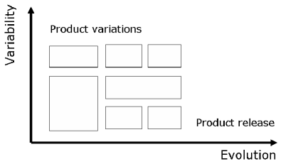
Svahnberg studies the relationship between variability and evolution, as shown in Figure 1.1, where product variations and product release span two dimensions. As his figure suggests, a set of products evolve over time just as one product does. Any extensibility mechanism which does not take these two dimensions into consideration can not fully provide satisfactory solutions.

In this thesis, we propose type safe extensible programming which takes two dimensions into consideration. In particular, our language provides extensibility mechanisms at multiple levels of granularity, from the fine degree (at the core expression level) to the coarse degree (at the module level). At the same time, in order to manage variability, we adopt product line engineering as a developing paradigm, and then provide a development process which guides how to apply this paradigm to our extensibility mechanisms:

  • A core language that supports polymorphic extensible records, first-class cases and type safe exception handling (Section 3);

  • A module system that supports separate compilation in the presence of the above features (Section 4);

  • A development process that supports the construction of a family of systems (Section 5).

Chapter 2 Related work

Extensible programming is a programming style that focuses on mechanisms to extend a base system with additional functionality. The main idea of extensible programming is to use the existing artifacts (e.g., code, documents, or binary executables) but extend them to fit new requirements and extensibility mechanisms take an important role in simplifying such activities. Building extensible systems has received attention because it is seen as a way to reduce the development cost by reusing the existing code base, not by developing them from scratch. Furthermore, nowadays software products need to support extensibility from the beginning since the current computing environment demands a high level of adaptability by software products. Extensible programming provides language features designed for extensibility in oder to simplify the construction of extensible systems. In the remainder of this section, we will study similar works that take extensibility and adaptability in software into consideration.

2.1 The extensible language approach

Software evolves by means of adding and/or replacing its functionality over time. Such extensibility has been studied extensively in the context of compilers and programming languages. Previous work on extensible compilers has proposed new techniques on how to easily add extensions to existing programming languages and their compilers. For example, JaCo is an extensible compiler for Java based on extensible algebraic types (Zenger and Odersky 2001, 2005). The Polyglot framework implements an extensible compiler where even changes of compilation phases and manipulation of internal abstract syntax trees are possible  (Nystrom et al. 2003). Aspect-oriented concepts are also applied to extensible compiler construction (Wu et al. 2005).

However, most of these existing solutions do not attempt to pay special attention to the set of extensions they produce. Extensions are best accomplished if the original code base was designed for extensibility. Even worse, successive extensions can make the code base difficult to learn and hard to change substantially. For example, the GNU Compiler Collection (GCC ) started as an efficient C compiler but has evolved to officially support more than seven programming languages and a large number of target architectures. However, a variety of source languages and target architectures have resulted in a complexity that makes it difficult to do GCC development (Vichare 2008). This effect apparently even led to some rifts within the GCC developer community (Matzan 2007).

2.2 The design patterns approach

In software engineering, extensibility is one kind of design principle where the goal is to minimize the impact of future changes on existing system functions. Therefore, it has become common practice to prepare for future changes when we design systems. The concept of Design patterns takes an important role in this context  (Gamma et al. 1995). Each pattern provides design alternatives which take changes into consideration so that the system is robust enough to accommodate such changes. For example, the visitor pattern makes it easy to define a new operation without changing the classes of the members on which it is performed. It is particularly useful when the classes defining the object structure rarely change. By clearly defining intent, applicability and consequences of their application, patterns will help programmers manage changes.

However, design patterns are not generally applicable to non-object-oriented languages. Even worse, Norvig shows how it is trivial to implement various design patterns in dynamic languages (Norvig 1998). Some criticize that design patterns are just workarounds for missing language features (Monteiro 2006).

2.3 The feature-oriented programming approach

Product line engineering is an emerging paradigm for construction of a family of products (Kang et al. 2002; Lee et al. 2002; SEI 2008). This paradigm encourages developers to focus on developing a set of products rather than on developing one particular product. Therefore, mechanisms for managing variability through the design and implementation phases are essential. While most efforts in product line engineering have focused on principles and guidelines, only a few have suggested concrete mechanisms of implementing variations. Consequently, their process-centric approach is too abstract to provide a working solution in a particular language. For example, the Feature-Oriented Reuse Method (FORM) often suggests parameterization techniques, but implementation details are left to developers (Kang et al. 1998; Lee et al. 2000). Therefore, preprocessors, e.g., macro systems, have been used in many examples in the literature as the feature delivery method (Kang et al. 1998, 2005). For example, the macro language in FORM determines inclusion or exclusion of some code segments based on the feature selection. Macro languages have some advantage in that they can be mixed easily with any target programming languages, however, feature specific segments are scattered across multiple classes, so code can easily become complicated. Even worse, since general purpose compilers do not understand the macro language, any error appearing in feature code segments cannot be detected until all feature sets are selected and the corresponding code segments are compiled.

In order to take advantage of the current compiler technology including static typing and separate compilation, we need native language support. Therefore, feature-oriented programming emerges as an attempt to provide better support for feature modularity (Lopez-Herrejon et al. 2005). FeatureC++ (Apel et al. 2005) and AHEAD (Batory 2004) are such language extensions to C++ and Java, respectively. In these approaches, features are implemented as distinct units and then they are combined to become a product. However, there still is no formal type system, so these languages do not guarantee the absence of type errors during feature composition (Thaker et al. 2007). Recently, such a formal type system has been proposed for a simple, experimental feature-oriented language (Apel et al. 2008).

2.4 The generic programming approach

The idea of generic programming is to implement the common part once and parameterize variations so that different products can be instantiated by assigning distinct values as parameters. Higher-order modules, also known as functors – e.g., in the Standard ML programming language (SML), are a typical example in that they can be parameterized on values, types and even other modules, possibly including higher-order ones (Appel and MacQueen 1991). The SML module system has been demonstrated to be powerful enough to manage variations in the context of product lines (Chae and Blume 2008).

However, its type system sometimes impose restrictions which require code duplication between functions on data types. Many proposals to overcome this restriction have been presented. For example, MLPolyR proposes extensible cases (Blume et al. 2006), and OCaml proposes polymorphic variants (Garrigue 2000).

Similarly, templates in C++ provide parameterization over types and have been extensively studied in the context of programming families  (Czarnecki and Eisenecker 2000). Recently, an improvement that would provide better support of generic programming has been proposed (Dos Reis and Stroustrup 2006). Originally, Java and C# did not support parameterized types but now both support similar concepts (Torgersen 2004; Garcia et al. 2007).

Sometimes the generic programming approach is criticized for its difficulty in identifying variation points and defining parameters (Gacek and Anastasopoules 2001). However, systematic reasoning (e.g., product line analysis done by product line architects) can ease this burden by providing essential information for product line implementation  (Chae and Blume 2008).

2.5 The generative programming approach

Generative programming is a style of programming that utilizes code generation techniques which make it possible to generate code from generic artifacts such as specifications, diagrams, and templates (Czarnecki 2004). This approach is similar to the generic programming approach in that a specialized program can be obtained from a generic one, but the generative programming approach focuses on the usage of domain specific languages and their code generators while the generic programming approach focuses on the usage of the built-in language features such as templates and functors.

2.6 The open programming approach

Extensions can be added generally by modifying source code. In this compile-time form of extensions, a program needs to be compiled for extensions to become available. However, in some cases, a software product need to modify its behavior dynamically during its execution. Non-stop applications are such examples. Sometimes, a certain type of change can be arranged to be picked up by a linker during load-time. Open programming is an attempt at addressing these issues in the context of programming languages. For instances, Java can dynamically load (class-) libraries for this sort of thing. Rossberg proposes the Alice ML programming language which reconciles open programming concepts with strong typing (Rossberg 2007).

Similarly, there have been attempts to upgrade software while it is running. Appel illustrated the usage of “applicative” module linking to demonstrate how to replace a software module without having the downtime (Appel 1994). However, it was Erlang that made this “hot-sliding” or “hot code swapping” idea popular (Armstrong 2007). In Erlang, old code can be phased out and replaced by new code, which makes it easier to fix bugs and upgrade a running system.

Unlike these approaches, we focus on compile-time extensions by modifying source code with minimal efforts.

Chapter 3 Type safe extensible programming

3.1 Introduction

The MLPolyR language has been specifically designed to support type-safe extensible programming at a relatively fine degree of granularity. Its records are polymorphic and extensible unlike in most programming languages where records must be explicitly declared and are not extensible. As their duals, polymorphic sums with extensible cases make composable extensions possible. Moreover, by taking advantage of representing exceptions as sums and assigning exception handlers polymorphic, extensible row types, we can provide type-safe exception handling, which suggests “well-typed programs do not have uncaught exceptions.”

To understand the underlying mechanism, it is instructive to first look at an example. The following sections informally provide such examples that highlight the extensible aspect of the MLPolyR language. Then, we show how these constructors provide a solution to the expression problem which is considered one of the most fundamental problems in the study of extensibility (Section 3.2).

Theoretical aspects of this language (derived from the previously published conference papers  (Blume et al. 2006, 2008)) are presented in the following sections. First, we consider an implicitly typed external language $\mathsf{EL}$ that extends $\lambda$-calculus with polymorphic extensible records, extensible cases and exceptions. Our implementation rests on a deterministic, type sensitive semantics for $\mathsf{EL}$ based on elaboration (i.e., translation) into an explicitly typed internal language $\mathsf{IL}$. The elaboration process involves type inference for $\mathsf{EL}$. Our compiler for MLPolyR provides efficient type reconstruction of principal types by using a variant of the well-known algorithm W (Milner 1978a). Finally, $\mathsf{IL}$ is translated into a variant of an untyped language, called LRec, which is closer to machine code. Therefore, our compiler is structured as follows:

𝖤𝖫Section3.3𝖨𝗆𝗉𝗅𝖼𝗂𝗍𝗅𝗒𝗍𝗒𝗉𝖾𝖽𝖢𝖯𝖲𝖺𝗇𝖽𝖣𝗎𝖺𝗅𝗍𝗋𝖺𝗇𝗌𝖿𝗈𝗋𝗆𝖺𝗍𝗂𝗈𝗇𝖨𝖫Section3.4𝖤𝗑𝗉𝗅𝗂𝖼𝗂𝗍𝗅𝗒𝗍𝗒𝗉𝖾𝖽𝖨𝗇𝖽𝖾𝗑𝖯𝖺𝗌𝗌𝗂𝗇𝗀𝖫𝖱𝖾𝖼Section3.5𝖴𝗇𝗍𝗒𝗉𝖾𝖽λ𝖼𝖺𝗅𝖼𝗎𝗅𝗎𝗌superscript𝖢𝖯𝖲𝖺𝗇𝖽𝖣𝗎𝖺𝗅𝗍𝗋𝖺𝗇𝗌𝖿𝗈𝗋𝗆𝖺𝗍𝗂𝗈𝗇subscriptsuperscriptabsent𝖤𝖫superscriptsuperscript𝑆𝑒𝑐𝑡𝑖𝑜𝑛3.3𝖨𝗆𝗉𝗅𝖼𝗂𝗍𝗅𝗒𝗍𝗒𝗉𝖾𝖽subscriptsuperscriptabsent𝖨𝖫superscriptsuperscript𝑆𝑒𝑐𝑡𝑖𝑜𝑛3.4𝖤𝗑𝗉𝗅𝗂𝖼𝗂𝗍𝗅𝗒𝗍𝗒𝗉𝖾𝖽superscript𝖨𝗇𝖽𝖾𝗑𝖯𝖺𝗌𝗌𝗂𝗇𝗀subscriptsuperscriptabsent𝖫𝖱𝖾𝖼superscriptsuperscript𝑆𝑒𝑐𝑡𝑖𝑜𝑛3.5𝖴𝗇𝗍𝗒𝗉𝖾𝖽𝜆𝖼𝖺𝗅𝖼𝗎𝗅𝗎𝗌\underbrace{\stackrel{{\scriptstyle\mathsf{EL}}}{{~{}}}}_{\stackrel{{\scriptstyle\mathsf{Implcitly~{}typed}}}{{\stackrel{{\scriptstyle\vdots}}{{Section~{}\ref{sec:el}}}}}}\stackrel{{\scriptstyle\mathsf{CPS~{}and~{}Dual~{}transformation}}}{{\vector(1,0){100.0}}}\underbrace{\stackrel{{\scriptstyle\mathsf{IL}}}{{~{}}}}_{\stackrel{{\scriptstyle\mathsf{Explicitly~{}typed}}}{{\stackrel{{\scriptstyle\vdots}}{{Section~{}\ref{sec:il}}}}}}\stackrel{{\scriptstyle\mathsf{Index~{}Passing}}}{{\vector(1,0){80.0}}}\underbrace{\stackrel{{\scriptstyle\mathsf{LRec}}}{{~{}}}}_{\stackrel{{\scriptstyle\mathsf{Untyped~{}\lambda-calculus}}}{{\stackrel{{\scriptstyle\vdots}}{{Section~{}\ref{sec:lrec}}}}}}

3.1.1 Polymorphic extensible records

MLPolyR supports polymorphic extensible records. One of its record expressions has the form { a = e, ... = $r$ }. This creates a new record which extends record r with a new field a. Table 3.1 shows more such record operations. Record update and renaming operations can be derived by combining extension and subtraction operations.

𝖲𝖾𝗅𝖾𝖼𝗍𝗂𝗈𝗇𝗏𝖺𝗅sel_a:β:{a}.{a:τ,β}{τ}𝐟𝐮𝐧sel_ar=r.a𝖤𝗑𝗍𝖾𝗇𝗌𝗂𝗈𝗇𝗏𝖺𝗅add_a:β:{a}.{β}{a:𝗂𝗇𝗍,β}𝐟𝐮𝐧add_ar={a=1,=r}𝖲𝗎𝖻𝗍𝗋𝖺𝖼𝗍𝗂𝗈𝗇𝗏𝖺𝗅sub_a:β:{a}.α.{a:α,β}{β}𝐟𝐮𝐧sub_a{a=_,=r}=r𝖴𝗉𝖽𝖺𝗍𝖾𝗏𝖺𝗅upd_a:β:{a}.α.{a:α,β}{a:𝗂𝗇𝗍,β}𝐟𝐮𝐧upd_ar=𝐥𝐞𝐭{a=_,=rest}=r𝐢𝐧{a=1,=rest}𝖱𝖾𝗇𝖺𝗆𝖾𝗏𝖺𝗅ren_a:β:{a,b}.α.{a:α,β}{b:α,β}𝐟𝐮𝐧ren_ar=𝐥𝐞𝐭{a=a,=rest}=r𝐢𝐧{b=a,=rest}\begin{array}[]{|@{~~}l@{~~~~}||@{~~~~}l|l|}\hline\cr{}~{}\lx@intercol\mathsf{Selection}\hfil~{}~{}~{}~{}\vrule\vrule~{}~{}~{}~{}&\mathsf{val}~{}sel\_a~{}:~{}\forall\beta:\left\{{a}\right\}.\left\{{a:\tau,\beta}\right\}\rightarrow\left\{{\tau}\right\}\\ {}~{}\lx@intercol\hfil~{}~{}~{}~{}\vrule\vrule~{}~{}~{}~{}&\mathbf{fun}~{}{sel\_a}~{}{r}={r.a}\\ \hline\cr{}~{}\lx@intercol\mathsf{Extension}\hfil~{}~{}~{}~{}\vrule\vrule~{}~{}~{}~{}&\mathsf{val}~{}add\_a~{}:~{}\forall\beta:\left\{{a}\right\}.\left\{{\beta}\right\}\rightarrow\left\{{a:\mathsf{int},\beta}\right\}\\ {}~{}\lx@intercol\hfil~{}~{}~{}~{}\vrule\vrule~{}~{}~{}~{}&\mathbf{fun}~{}{add\_a}~{}{r}={\mathbf{\{}{a=1,\ldots=r}\mathbf{\}}}\\ \hline\cr{}~{}\lx@intercol\mathsf{Subtraction}\hfil~{}~{}~{}~{}\vrule\vrule~{}~{}~{}~{}&\mathsf{val}~{}sub\_a~{}:~{}\forall\beta:\left\{{a}\right\}.\forall\alpha.\mathbf{\{}{a:\alpha,\beta}\mathbf{\}}\rightarrow\left\{{\beta}\right\}\\ {}~{}\lx@intercol\hfil~{}~{}~{}~{}\vrule\vrule~{}~{}~{}~{}&\mathbf{fun}~{}{sub\_a}~{}{\mathbf{\{}{a=\_,\dots=r}\mathbf{\}}}={r}\\ \hline\cr{}~{}\lx@intercol\mathsf{Update}\hfil~{}~{}~{}~{}\vrule\vrule~{}~{}~{}~{}&\mathsf{val}~{}upd\_a~{}:~{}\forall\beta:\left\{{a}\right\}.\forall\alpha.\mathbf{\{}{a:\alpha,\beta}\mathbf{\}}\rightarrow\left\{{a:\mathsf{int},\beta}\right\}\\ {}~{}\lx@intercol\hfil~{}~{}~{}~{}\vrule\vrule~{}~{}~{}~{}&\mathbf{fun}~{}{upd\_a}~{}{r}={\mathbf{let}~{}{\mathbf{\{}{a=\_,\dots=rest}\mathbf{\}}}={r}~{}\mathbf{in}~{}{\mathbf{\{}{a=1,\ldots=rest}\mathbf{\}}}}\\ \hline\cr{}~{}\lx@intercol\mathsf{Rename}\hfil~{}~{}~{}~{}\vrule\vrule~{}~{}~{}~{}&\mathsf{val}~{}ren\_a~{}:~{}\forall\beta:\left\{{a,b}\right\}.\forall\alpha.\mathbf{\{}{a:\alpha,\beta}\mathbf{\}}\rightarrow\left\{{b:\alpha,\beta}\right\}\\ {}~{}\lx@intercol\hfil~{}~{}~{}~{}\vrule\vrule~{}~{}~{}~{}&\mathbf{fun}~{}{ren\_a}~{}{r}={\mathbf{let}~{}{\mathbf{\{}{a=a^{\prime},\dots=rest}\mathbf{\}}}={r}~{}\mathbf{in}~{}{\mathbf{\{}{b=a^{\prime},\ldots=rest}\mathbf{\}}}}\\ \hline\cr\end{array}
Table 3.1: Basic operations on records in MLPolyR.

To understand the extension mechanism, let us first look at an example. Since records are first-class values, we can abstract over the record being extended and obtain a function add_a that extends any argument record (as long as it does not already contain a) with a field a. Such a function can be thought of as the “difference” between its result and its argument:

fun add_a r = { a = 1, = r }

Here the difference consists of a field labeled a of type int and value 1. The type of function add_a is inferred as $\forall\beta:\left\{{a}\right\}.\left\{{\beta}\right\}\rightarrow\left\{{a:\mathsf{int},\beta}\right\}$ where $\beta:\left\{{a}\right\}$ represents a constraint that a row variable $\beta$ must not contain a label $a$. We can write similar functions add_b and add_c which add fields b of type $\mathsf{bool}$ and c of type $\mathsf{string}$ respectively:

fun add_b r = { b = true, = r }
fun add_c r = { c = hello”, = r }

We can then “add up” record differences represented by add_a, add_b, add_c by composing these functions:

fun add_ab r = add_a (add_b r)
fun add_bc r = add_b (add_c r)

where the inferred types are respectively:

$$\begin{array}[]{ll}\mathsf{val~{}add\_ab:~{}}&\forall\beta:\left\{{a,b}\right\}.\left\{{\beta}\right\}\rightarrow\left\{{a:\mathsf{int},b:\mathsf{bool},\beta}\right\}\\ \mathsf{val~{}add\_bc:~{}}&\forall\beta:\left\{{b,c}\right\}.\left\{{\beta}\right\}\rightarrow\left\{{b:\mathsf{bool},c:\mathsf{string},\beta}\right\}\end{array}$$

Finally, we can create actual records by “adding” differences to the empty record:

val a = add_a {}
val ab = add_ab {}
val bc = add_bc {}

Records as classes

Extensible records continue to receive attention since they can also be used as a type-theoretical basis for object-oriented programming (Rémy and Vouillon 1998). For example, assuming polymorphic records and references in place, we can define a base class, and then create sub-classes with additional methods in order to obtain the same effect of code reuse via inheritance.

As a demonstration of records as classes (followed by Pierce’s encoding (Pierce 2002)), we first define a $\mathsf{counter}$ class which provides two methods: 1) $\mathsf{get}$ returns the current value of a field $i$ by dereferencing and 2) $\mathsf{inc}$ increments its value by first reading and then assigning its incremental) as follows:

val counterClass = fn x =>
{get = fn _ => x!i,
inc = fn _ => x!i := x!i + 1
}

where $!$ is a dereferencing operator and $:=$ is an assignment operator. Then, individual $\mathsf{counter}$ objects can be obtained by a counter generator $\mathsf{newCounter}$ which applies $\mathsf{counterClass}$ to a record with a reference field $i$:

val newCounter = fn _ => let
val x = {| i = 0 |}
in counterClass x
end

where $\{|\ldots|\}$ denotes a mutable record. Furthermore, by taking advantage of extensible records, we can implement a subclass $\mathsf{resetCounterClass}$ which extends the base class $\mathsf{counterClass}$ with a new method $\mathsf{reset}$ like this:

val resetCounterClass = fn x =>
{…=counterClass x,
reset = fn _ => x!i := 0
}

where $\ldots$ refers to the same fields that the base class contains, so the returned value contains one more field named $\mathsf{reset}$. Similarly, individual $\mathsf{resetCounter}$ objects can be obtained by a generator $\mathsf{newResetCounter}$:

val newResetCounter = fn _ => let
val x = {| i= 0 |}
in resetCounterClass x
end

3.1.2 Extensible programming with first-class cases

Variants are dual of records in the same manner as logical $\vee$ is dual to $\wedge$:

$$\begin{array}[]{c@{~~}c@{~~}c}\neg{\mathbf{\{}{a\wedge b}\mathbf{\}}}\hfil~{}~{}&=\hfil~{}~{}&\left<\neg a\vee\neg b\right>\\ \neg\left<a\vee b\right>\hfil~{}~{}&=\hfil~{}~{}&\mathbf{\{}{\neg a\wedge\neg b}\mathbf{\}}\\ \end{array}$$

Then, as in any dual construction, the introduction form of the primal corresponds to the elimination form of the dual. Thus, elimination forms of sums (e.g., match) correspond to introduction forms of records. In particular, record extension (an introduction form) corresponds to the extension of cases (an elimination form). This duality motivates making cases first-class values as opposed to a mere syntactic form. With cases being first-class and extensible, one can use the usual mechanisms of functional abstraction in a style of programming that facilitates composable extensions.

Here is a function representing the difference between two code fragments, one of which can handle case ‘A while the other, represented by the argument $c$, cannot:

fun add_A c = cases A () => print A
default: c

where data type constructors ($`A~{}()$) are represented by prefixing their names with a backquote character ‘. Note that function add_A corresponds to add_a of the dual (in Section 3.1.1). The type inferred for add_A is $\forall\beta:\left\{{`A}\right\}.({\left<{\beta}\right>}\hookrightarrow{()})\rightarrow({\left<{`A:(),\beta}\right>}\hookrightarrow{()})$ where a type ${\left<{\rho}\right>}\hookrightarrow{\tau}$ denotes the type of first-class cases, $\left<{\rho}\right>$ is the sum type that is being handled, and $\tau$ is the result. We also assume that $()$ denotes a unit type.

Examples for functions add_B and add_C (corresponding to add_b and add_c in the dual) are:

fun add_B c = cases B () => print B
default: c
fun add_C c = cases C () => print C
default: c

As in the dual, we can now compose difference functions to obtain larger differences:

fun add_AB c = add_A (add_B c)
fun add_BC c = add_B (add_C c)

By applying a difference to the empty case nocases we obtain case values:

val case_A = add_A nocases
val case_AB = add_AB nocases
val case_BC = add_BC nocases

These values can be used in a match form. The match construct is the elimination form for the case arrow $\hookrightarrow$. The following expression will cause "B" to be printed:

match B () with case_BC

The previous examples demonstrate how functional record extension in the primal corresponds to code extension in the dual. The latter feature gives rise to a simple programming pattern facilitating composable extensions. Composable extensions can be used as a principled approach to solving the well-known expression problem described by Wadler (Wadler 1998). We will show how our composable extensions provide a solution to the expression problem in the following section (Section 3.2).

3.1.3 Exception handlers as extensible cases

Exceptions are an indispensable part of modern programming languages. They are, however, handled poorly, especially by higher-order languages such as ML and Haskell: in both languages a well-typed program can unexpectedly fail due to an uncaught exception. MLPolyR enriches the type system with type-safe exception handling by relying on representing exceptions as sums and assigning exception handlers polymorphic, extensible row types. Our syntax distinguishes between the act of establishing a new exception handler ($\mathbf{handle}$) and that of overriding an existing one ($\mathbf{rehandle}$). The latter can be viewed as a combination of $\mathbf{unhandle}$ (which removes an existing handler) and $\mathbf{handle}$. This design choice makes it possible to represent exception types as row types without need for additional complexity. From a usability perspective, the design makes overriding a handler explicit, reducing the likelihood of this happening by mistake.

We will now visit a short sequence of simple program fragments, roughly ordered by increasing complexity. None of the examples exhibits uncaught exceptions. The rejection of any one of them by a compiler would constitute a false positive. The type system and the compiler that we describe accept them all.

Of course, baseline functionality consists of being able to match a manifest occurrence of a raised exception with a manifestly matching handler:

(… raise Neg 10 …) handle Neg i =>

The next example moves the site where the exception is raised into a separate function. To handle this in the type system, the function type constructor $\rightarrow$ acquires an additional argument $\rho$ representing the set of exceptions that may be raised by an application, i.e., function types have the form $\tau_{1}\stackrel{{\scriptstyle\rho}}{{\rightarrow}}\tau_{2}$. This is about as far as existing static exception trackers that are built into programming languages (e.g., Java’s throws declaration) go.

fun foo x = if x < 0 then raise Neg x else
(… foo y …) handle Neg i => x

But we also want to be able to track exceptions through calls of higher-order functions such as map, which themselves do not raise exceptions while their functional arguments might:

fun map f [] = []
| map f (x::xs) = f x :: map f xs
(… map f l …) handle Neg i =>

Moreover, in the case of curried functions and partial applications, we want to be able to distinguish stages that do not raise exceptions from those that might. In the example of map, there is no possibility of any exception being raised when map is partially applied to the function argument; all exceptions are confined to the second stage when the list argument is supplied:

val mfoo = map foo
(… mfoo l …) handle Neg i =>

Here, the result mfoo of the partial application acts as a data structure that carries a latent exception. In the general case, exception values can occur in any data structure. For example, the SML/NJ Library (Gansner and Reppy 2002) provides a constructor function for hash tables which accepts a programmer-specified exception value which becomes part of the table’s representation from where it can be raised, for example when an attempt is made at looking up a non-existing key.

The following example shows a similar but simpler situation. Function check finds the first pair in the given list whose left component does not satisfy the predicate ok. If such a pair exists, its right component, which must be an exception value, is raised. To guarantee exception safety, the caller of check must be prepared to handle any exception that might be passed along in the argument of the call:

fun check ((x, e)::rest) = if ok x then check rest else raise e
| check [] = ()
(… check [(3, A 10), (4, B true)] …) handle A i =>
| B b =>

Finally, exception values can participate in complex data flow patterns. The following example illustrates this by showing an exception ‘A that carries another exception ‘B as its payload. The payload ‘B 10 itself gets raised by the exception handler for ‘A in function f2, so a handler for ‘B on the call of f2 suffices to make this fragment exception-safe:

fun f1 () = raise A (‘B 10)
fun f2 () = f1 () handle A x => raise x
(… f2 () …) handle B i =>

3.2 Case study: A two-way extensible interpreter

There are two axes along which we can extend a system: functionality and variety of data. For the first axis, we can add more functionality on the basic set of data. For the second axis, we can add to the variety of data on which the basic functions perform. Ideally, two dimensional extensions should be orthogonal. However, depending on the context, extensions along one axis can be more difficult than along the other. Simultaneous two-way extensions can be even more difficult. This phenomenon can be easily explained in terms of expressions (data) and evaluators (functions), which the reason Wadler called it the expression problem (Wadler 1998). This section discusses a two-way extensible interpreter that precisely captures this phenomenon. Our intention with this case study is to define a real yet simple example that extends its functionality in an interesting way.

Base language

Let us consider a Simple Arithmetic Language (SAL) that contains terms such as numbers, variables, additions, and a let-binding form. Not all expressions that conform to the grammar are actually “good” expressions. We want to reject expressions that have “dangling” references to variables which are not in scope. The judgment $\Gamma\vdash e~{}\mbox{\bf ok}~{}$ expresses that $e$ is an acceptable expression if it appears in a context described by $\Gamma$. In this simple case, $\Gamma$ keeps track of which variables are currently in scope, so we take it to be a set of variables. An expression is acceptable as a program if it is an expression that makes no demands on its context, i.e., $\varnothing\vdash e~{}\mbox{\bf ok}~{}$. When discussing the dynamic semantics of a language, we need to define its values, i.e., the results of a computation. In SAL, values are simply natural numbers. Then, our evaluation semantics describes the entire evaluation process as one “big step”. We write $(E,e)\Downarrow n$ to say that $e$ evaluates to $n$ under environment $E$. The environment is a finite mapping from variables to values.

$\mathsf{Values}~{}~{}~{}~{}n\in N$
$\mathsf{Variables}~{}x\in Var$
$\mathsf{Terms}~{}~{}~{}~{}~{}e\mathrel{\colon\!\!\!\colon\!\!\mathord{=}}n\mathrel{\mid}x\mathrel{\mid}e+e\mathrel{\mid}\mathbf{let}~{}{x}={e}~{}\mathbf{in}~{}{e}$
  $\Gamma\vdash e~{}\mbox{\bf ok}~{}$

$\mathsf{Typing~{}env.}~{}\Gamma\mathrel{\colon\!\!\!\colon\!\!\mathord{=}}\varnothing\mathrel{\mid}\Gamma,x$

  $\displaystyle\displaystyle{\hbox{}\over\hbox{\hskip 20.42828pt\vbox{\vbox{}\hbox{\hskip-20.42828pt\hbox{\hbox{$\displaystyle\displaystyle{\Gamma\vdash n~{}\mbox{\bf ok}~{}}$}}}}}}$        $\displaystyle\displaystyle{\hbox{\hskip 12.0937pt\vbox{\hbox{\hskip-12.09369pt\hbox{\hbox{$\displaystyle\displaystyle{x\in\Gamma}$}}}\vbox{}}}\over\hbox{\hskip 20.28474pt\vbox{\vbox{}\hbox{\hskip-20.28474pt\hbox{\hbox{$\displaystyle\displaystyle{\Gamma\vdash x~{}\mbox{\bf ok}~{}}$}}}}}}$        $\displaystyle\displaystyle{\hbox{\hskip 52.3105pt\vbox{\hbox{\hskip-52.3105pt\hbox{\hbox{$\displaystyle\displaystyle{\Gamma\vdash e_{1}~{}\mbox{\bf ok}~{}}$}\hskip 20.00003pt\hbox{\hbox{$\displaystyle\displaystyle{\Gamma\vdash e_{2}~{}\mbox{\bf ok}~{}}$}}}}\vbox{}}}\over\hbox{\hskip 29.88336pt\vbox{\vbox{}\hbox{\hskip-29.88336pt\hbox{\hbox{$\displaystyle\displaystyle{\Gamma\vdash e_{1}+e_{2}~{}\mbox{\bf ok}~{}}$}}}}}}$        $\displaystyle\displaystyle{\hbox{\hskip 56.8348pt\vbox{\hbox{\hskip-56.83478pt\hbox{\hbox{$\displaystyle\displaystyle{\Gamma\vdash e_{1}~{}\mbox{\bf ok}~{}}$}\hskip 20.00003pt\hbox{\hbox{$\displaystyle\displaystyle{\Gamma,x\vdash e_{2}~{}\mbox{\bf ok}~{}}$}}}}\vbox{}}}\over\hbox{\hskip 47.7359pt\vbox{\vbox{}\hbox{\hskip-47.7359pt\hbox{\hbox{$\displaystyle\displaystyle{\Gamma\vdash\mathbf{let}~{}{x}={e_{1}}~{}\mathbf{in}~{}{e_{2}}~{}\mbox{\bf ok}~{}}$}}}}}}$

  $(E,e)\Downarrow n$

$\mathsf{Environment}~{}E\in\mathsf{Var}\rightarrow N$

  $\displaystyle\displaystyle{\hbox{\hskip 20.39348pt\vbox{\hbox{\hskip-20.39348pt\hbox{\hbox{$\displaystyle\displaystyle{E(x)=n}$}}}\vbox{}}}\over\hbox{\hskip 21.78235pt\vbox{\vbox{}\hbox{\hskip-21.78233pt\hbox{\hbox{$\displaystyle\displaystyle{(E,x)\Downarrow n}$}}}}}}$        $\displaystyle\displaystyle{\hbox{\hskip 90.18698pt\vbox{\hbox{\hskip-90.18698pt\hbox{\hbox{$\displaystyle\displaystyle{(E,e_{1})\Downarrow n_{1}}$}\hskip 20.00003pt\hbox{\hbox{$\displaystyle\displaystyle{(E,e_{2})\Downarrow n_{2}}$}\hskip 20.00003pt\hbox{\hbox{$\displaystyle\displaystyle{n_{1}+n_{2}=n}$}}}}}\vbox{}}}\over\hbox{\hskip 31.38097pt\vbox{\vbox{}\hbox{\hskip-31.38095pt\hbox{\hbox{$\displaystyle\displaystyle{(E,e_{1}+e_{2})\Downarrow n}$}}}}}}$        $\displaystyle\displaystyle{\hbox{}\over\hbox{\hskip 21.92589pt\vbox{\vbox{}\hbox{\hskip-21.92587pt\hbox{\hbox{$\displaystyle\displaystyle{(E,n)\Downarrow n}$}}}}}}$        $\displaystyle\displaystyle{\hbox{\hskip 73.42001pt\vbox{\hbox{\hskip-73.42001pt\hbox{\hbox{$\displaystyle\displaystyle{(E,e_{1})\Downarrow n_{1}}$}\hskip 20.00003pt\hbox{\hbox{$\displaystyle\displaystyle{(E[x\rightarrow n_{1}],e_{2})\Downarrow n_{2}}$}}}}\vbox{}}}\over\hbox{\hskip 51.18904pt\vbox{\vbox{}\hbox{\hskip-51.18904pt\hbox{\hbox{$\displaystyle\displaystyle{(E,\mathbf{let}~{}{x}={e_{1}}~{}\mathbf{in}~{}{e_{2}})\Downarrow n_{2}}$}}}}}}$
Figure 3.1: The Simple Arithmetic Languages (SAL): syntax (top), the static semantics (2nd) and the evaluation semantics (bottom).

Figure 3.2 shows a simple implementation for the base interpreter which is the composition of the function $\mathsf{check}$ (realizing the static semantics) and $\mathsf{eval}$ (realizing the evaluation semantics). As explained in Section 3.1.2, our language MLPolyR has polymorphic sum types. The type system is based on Rémy-style row polymorphism, handles equi-recursive types, and can infer principal types for all language constructs. For function $\mathsf{eval}$ in Figure 3.2, the compiler calculates the following type.

val eval:
$\forall\beta:\varnothing$. (($\alpha$ as <‘Let of (string, $\alpha$, $\alpha$),
‘Num of int,
‘Plus of ($\alpha$, $\alpha$),
‘Var of string>), string $\stackrel{{\scriptstyle\beta}}{{\rightarrow}}$ int) $\stackrel{{\scriptstyle\beta}}{{\rightarrow}}$ int

Here $\alpha$ is a recursive sum type, indicated by keyword as and a type row closed in < $\ldots$ >. $\beta$ is a row type variable constrained to a particular kind representing a set of labels that must be absent in any instantiation.

(* environment *)
fun bind (a, x, env) y =
if String.compare (x, y) == 0 then a else env y
fun empty x =
raise Fail (String.concat [“unbound variable: “, x, “\n”])
(* the static semantics *)
(* check returns () or fails with Fail *)
fun check (e, env) = match e with
cases Var x => env x
| Num n => ()
| Plus (e1, e2) => (check (e1, env); check (e2, env))
| Let (x, e1, e2) => (check (e1, env);
check (e2, bind ((), x, env))
(* the evaluation semantics *)
fun eval (e, env) = match e with
cases Var x => env x
| Num n => n
| Plus (e1, e2) => eval (e1, env) + eval (e2, env)
| Let (x, e1, e2) =>
eval (e2, bind (eval (e1, env), x, env))
(* the interpreter obtained by composing two functions *)
fun interp e =
try r = (check (e, empty); eval (e, empty))
in r
handling Fail msg => (String.output msg; -1)
end
Figure 3.2: A simple implementation for the base interpreter.

Preparation for extensions

Because it is desirable to extend the base language by new language features, we had better prepare for language extensions. In MLPolyR, first-class extensible cases can be helpful to make code extensible. Case expressions have an elimination form, $\mathbf{match}~{}{e_{1}}~{}{\mathbf{with}}~{}{e_{2}}$ where $e_{1}$ is a scrutinee and $e_{2}$ is a case expression. First, we separate cases from the scrutinee in the $\mathbf{match}$ expression. Then, we parameterize them by closing over their free variables. One of these free variables is the recursive instance of the current function itself. This design achieves open-recursion. With this setting, it becomes easy to add a new variant (i.e., new cases). For example, Figure 3.3 shows the old function $\mathsf{check}$ becomes a pair of $\mathsf{check}$_$\mathsf{case}$ and $\mathsf{check}$. The new version of $\mathsf{eval}$ follows the same pattern. For $\mathsf{eval\_case}$, the compiler calculates the following type and here it shows that its return type is the case type denoted by $\left<{\rho}\right>\stackrel{{\scriptstyle}}{{\hookrightarrow}}\tau$:

val eval_case:
$\forall\beta:\varnothing$. (($\alpha$, string $\stackrel{{\scriptstyle\beta}}{{\rightarrow}}$ int) $\stackrel{{\scriptstyle\beta}}{{\rightarrow}}$ int, string $\stackrel{{\scriptstyle\beta}}{{\rightarrow}}$ int) $\rightarrow$
(<‘Let of (string, $\alpha$, $\alpha$),
‘Num of int,
‘Plus of ($\alpha$, $\alpha$),
‘Var of string>) $\stackrel{{\scriptstyle\beta}}{{\hookrightarrow}}$ int)
(* extensible cases for the static semantics *)
fun check_case (check, env) =
cases Var x => env x
| Num n => ()
| Plus (e1, e2) => (check (e1, env); check (e2, env))
| Let (x, e1, e2) => (check (e1, env);
check (e2, bind ((), x, env))
(* close open recursion for the static semantics *)
fun check (e, env) = match e with check_case (check, env)
(* extensible cases for the evaluation semantics *)
fun eval_case (eval, env) =
cases Var x => env x
| Num n => n
| Plus (e1, e2) => eval (e1, env) + eval (e2, env)
| Let (x, e1, e2) =>
eval (e2, bind (eval (e1, env), x, env))
(* close open recursion for the evaluation semantics *)
fun eval (e, env) = match e with eval_case (eval, env)
Figure 3.3: Preparation for extensions.

$\mathsf{Terms}~{}~{}~{}~{}~{}e\mathrel{\colon\!\!\!\colon\!\!\mathord{=}}\ldots\mathrel{\mid}\mathbf{if0}~{}({e},{e},{e})$

  $\Gamma\vdash e~{}\mbox{\bf ok}~{}$

  $\displaystyle\displaystyle{\hbox{\hskip 83.46576pt\vbox{\hbox{\hskip-83.46576pt\hbox{\hbox{$\displaystyle\displaystyle{\Gamma\vdash e_{1}~{}\mbox{\bf ok}~{}}$}\hskip 20.00003pt\hbox{\hbox{$\displaystyle\displaystyle{\Gamma\vdash e_{2}~{}\mbox{\bf ok}~{}}$}\hskip 20.00003pt\hbox{\hbox{$\displaystyle\displaystyle{\Gamma\vdash e_{3}~{}\mbox{\bf ok}~{}}$}}}}}\vbox{}}}\over\hbox{\hskip 42.63762pt\vbox{\vbox{}\hbox{\hskip-42.63762pt\hbox{\hbox{$\displaystyle\displaystyle{\Gamma\vdash\mathbf{if0}~{}({e_{1}},{e_{2}},{e_{3}})~{}\mbox{\bf ok}~{}}$}}}}}}$

  $(E,e)\Downarrow n$

  $\displaystyle\displaystyle{\hbox{\hskip 56.20453pt\vbox{\hbox{\hskip-56.20453pt\hbox{\hbox{$\displaystyle\displaystyle{(E,e_{1})\Downarrow 0}$}\hskip 20.00003pt\hbox{\hbox{$\displaystyle\displaystyle{(E,e_{2})\Downarrow n_{2}}$}}}}\vbox{}}}\over\hbox{\hskip 46.09076pt\vbox{\vbox{}\hbox{\hskip-46.09076pt\hbox{\hbox{$\displaystyle\displaystyle{(E,\mathbf{if0}~{}({e_{1}},{e_{2}},{e_{3}}))\Downarrow n_{2}}$}}}}}}$        $\displaystyle\displaystyle{\hbox{\hskip 80.14575pt\vbox{\hbox{\hskip-80.14575pt\hbox{\hbox{$\displaystyle\displaystyle{(E,e_{1})\Downarrow n_{1}}$}\hskip 20.00003pt\hbox{\hbox{$\displaystyle\displaystyle{n_{1}\neq 0}$}\hskip 20.00003pt\hbox{\hbox{$\displaystyle\displaystyle{(E,e_{3})\Downarrow n_{3}}$}}}}}\vbox{}}}\over\hbox{\hskip 46.09076pt\vbox{\vbox{}\hbox{\hskip-46.09076pt\hbox{\hbox{$\displaystyle\displaystyle{(E,\mathbf{if0}~{}({e_{1}},{e_{2}},{e_{3}}))\Downarrow n_{3}}$}}}}}}$

  $(k,E,e)\Rightarrow(k^{\prime},E^{\prime},e^{\prime})~{}~{}~{}(k,E,e)\Rightarrow(n,k^{\prime})~{}~{}~{}(n,k)\Rightarrow(n^{\prime},k^{\prime})~{}~{}~{}(n,k)\Rightarrow(k^{\prime},E,e)$

$\mathsf{Frame}~{}~{}~{}f\mathrel{\colon\!\!\!\colon\!\!\mathord{=}}\left<{[]+e,E}\right>\mathrel{\mid}\left<{n+[]}\right>\mathrel{\mid}\left<{\mathbf{let}~{}{x}={[]}~{}\mathbf{in}~{}{e},E}\right>\mathrel{\mid}\left<{\mathbf{if0}~{}({[]},{e},{e})}\right>$
$\mathsf{Stack}~{}~{}~{}~{}k\mathrel{\colon\!\!\!\colon\!\!\mathord{=}}\cdot\mathrel{\mid}f\triangleright k$

$\displaystyle(k,E,x)\Rightarrow(E(x),k)\penalty 50\hskip 20.00003pt plus 0.5fil minus 5.0pt(k,E,n)\Rightarrow(n,k)\penalty 50\hskip 20.00003pt plus 0.5fil minus 5.0pt\penalty 50\hskip 20.00003pt plus 0.5fil minus 5.0pt(k,E,e_{1}+e_{2})\Rightarrow(\left<{[]+e_{2},E}\right>\triangleright k,E,e_{1})\penalty 50\hskip 20.00003pt plus 0.5fil minus 5.0pt(k,E,\mathbf{let}~{}{x}={e_{1}}~{}\mathbf{in}~{}{e_{2}})\Rightarrow(\left<{\mathbf{let}~{}{x}={[]}~{}\mathbf{in}~{}{e_{2}},E}\right>\triangleright k,E,e_{1})\penalty 50\hskip 20.00003pt plus 0.5fil minus 5.0pt(k,E,\mathbf{if0}~{}({e_{1}},{e_{2}},{e_{3}}))\Rightarrow(\left<{\mathbf{if0}~{}({[]},{e_{2}},{e_{3}}),E}\right>\triangleright k,E,e_{1})\penalty 50\hskip 20.00003pt plus 0.5fil minus 5.0pt(n,\left<{[]+e,E}\right>\triangleright k)\Rightarrow(\left<{n+[]}\right>\triangleright k,E,e)\penalty 50\hskip 20.00003pt plus 0.5fil minus 5.0pt(n,\left<{n^{\prime}+[]}\right>)\triangleright k)\Rightarrow(n^{\prime}+n,k)\penalty 50\hskip 20.00003pt plus 0.5fil minus 5.0pt(n,\left<{\mathbf{let}~{}{x}={[]}~{}\mathbf{in}~{}{e_{2}},E}\right>\triangleright k)\Rightarrow(k,E[x\rightarrow n],e_{2})\penalty 50\hskip 20.00003pt plus 0.5fil minus 5.0pt(0,\left<{\mathbf{if0}~{}({[]},{e_{2}},{e_{3}}),E}\right>\triangleright k)\Rightarrow(k,E,e_{2})\penalty 50\hskip 20.00003pt plus 0.5fil minus 5.0pt(n,\left<{\mathbf{if0}~{}({[]},{e_{2}},{e_{3}}),E}\right>\triangleright k)\Rightarrow(k,E,e_{3})~{}~{}~{}\mathsf{where}~{}~{}~{}n\neq 0$

  $e\gg e^{\prime}$

$\displaystyle{n_{1}+n_{2}\gg n;n=n_{1}+n_{2}}\penalty 50\hskip 20.00003pt plus 0.5fil minus 5.0pt{\mathbf{if0}~{}({0},{e_{2}},{e_{3}})\gg e_{2}}\penalty 50\hskip 20.00003pt plus 0.5fil minus 5.0pt{\mathbf{if0}~{}({n},{e_{2}},{e_{3}})\gg e_{3};n\neq 0}$
Figure 3.4: Language extensions: syntax (top), the static semantics (2nd), the evaluation semantics (3rd), the machine semantics (4th) and optimization rules (bottom).

Language extensions

Figure 3.4 shows how the base language grows. As a conditional term $\mathsf{If0}$ is introduced, the corresponding rule sets for both the static semantics ($\mathsf{check}$) and the evaluation semantics ($\mathsf{eval}$) are changed. Instead of the evaluation semantics, alternatively, we can define the machine semantics ($\mathsf{eval}_{\mathsf{m}}$) which makes control explicit by representing computation stages as stacks of frames. Each frame $f$ corresponds to a piece of work that has been postponed until a sub-computation is complete. Our machine semantics follows the conventional single-step transition rules between states (Harper 2005). It consists of expression states $(k,E,e)$, value states $(n,k)$ and a transition relation between states where $k$ is a stack and $e$ is the current expression. The empty stack is $\cdot$ and a frame $f$ on top of stack $k$ is written $f\triangleright k$. The machine semantics is given as a set of single-step transition rules $(k,E,e)\Rightarrow(k^{\prime},E^{\prime},e^{\prime})$ and $(n,k)\Rightarrow(n^{\prime},k^{\prime})$ between states. Additionally, optimization rules may be introduced. We write $e\gg e^{\prime}$ to say that $e$ is translated into $e^{\prime}$ by performing some simple optimization. In our running example, we consider constant folding and short-circuiting techniques.

Implementation of extensions

With our preparation for extensions in place, we only have to focus on a single new case ($\mathsf{`If0}$) by letting the original set of other cases be handled by $\mathsf{check}$_$\mathsf{case}$. Figure 3.5 shows how an extended checker $\mathsf{echeck}$, now handling five cases including $\mathsf{`If0}$, is obtained by closing the recursion through applying $\mathsf{echeck}$_$\mathsf{case}$ to $\mathsf{echeck}$ (Line 8). The extension of $\mathsf{eval}$, called $\mathsf{eeval}$, is constructed analogously by applying $\mathsf{eeval\_case}$ whose types is computed as follows:

val eeval_case:
$\forall\beta:\varnothing$. (($\alpha$, string $\stackrel{{\scriptstyle\beta}}{{\rightarrow}}$ int) $\stackrel{{\scriptstyle\beta}}{{\rightarrow}}$ int, string $\stackrel{{\scriptstyle\beta}}{{\rightarrow}}$ int) $\rightarrow$
(<‘If0 of ($\alpha$, $\alpha$, $\alpha$),
‘Let of (string, $\alpha$, $\alpha$),
‘Num of int,
‘Plus of ($\alpha$, $\alpha$),
‘Var of string>) $\stackrel{{\scriptstyle\beta}}{{\hookrightarrow}}$ int)

Finally, the extended interpreter can be obtained by applying $\mathsf{eeval}$ and $\mathsf{echeck}$, instead of $\mathsf{eval}$ and $\mathsf{check}$ (Line 22).

(* extends check_case with a new case (‘If0) *)
fun echeck_case (check, env) =
cases If0 (e1, e2, e3) =>
(check (e1, env); check (e2, env); check (e3, env))
default: check_case (check, env)
(* close open recursion with the extension *)
fun echeck (e, env) = match e with echeck_case (echeck, env)
(* extends eval_case with a new case (‘If0) *)
fun eeval_case (eval, env) =
cases If0 (e1, e2, e3) =>
if eval (e1, env) == 0
then eval (e2, env) else eval (e3, env)
default: eval_case (eval, env)
(* close open recursion with the extension *)
fun eeval (e, env) = match e with eeval_case (eeval, env)
(* the extended interpreter by composing extended functions *)
fun einterp e =
try r = (echeck (e, empty); eeval (e, empty))
in r
handling Fail msg => (String.output msg; -1)
end
Figure 3.5: Implementation for extensions.

Adding new kinds of functions such as a new optimizer ($\mathsf{opt}$) does not require any preparation in MLPolyR. For example, the combinator $\mathsf{opt}$ which performs constant folding may be inserted to build an optimized one:

(* the helper function for handling three cases *)
fun nope f = cases VAR x => f (‘VAR x)
| PLUS (e1, e2) => f (‘PLUS (e1, e2))
| LET (x, e1, e2) => f (‘LET (x, e1, e2))
(* PLUS (‘NUM n1, NUM n2) >> NUM (n1+n2) *)
(* otherwise, return arguments as received. *)
fun chkPLUS (e1, e2) = match e1 with
cases NUM n1 => (match e2 with
cases NUM n2 => NUM (n1+n2)
default: nope (fn _ => PLUS (e1, e2)))
default: nope (fn _ => PLUS (e1, e2))
(* the optimization rules *)
fun opt e = match e with
cases Var x => Var x
| Num n => Num n
| Plus (e1, e2) => chkPlus (opt e1, opt e2)
| Let (x, e1, e2) => Let (x, e1, e2)
(* the optimized interpreter by composing three functions *)
fun optimizedInterp e =
try r = (check (e, empty); eval (opt e, empty))
in r
handling Fail msg => (String.output msg; -1)
end

where we define a function $\mathsf{chkPlus}$ which returns $\mathsf{`Num(n_{1}+n_{2})}$ if two arguments are recursively optimized to $\mathsf{`Num(n_{1})}$ and $\mathsf{`Num(n_{2})}$, respectively. Otherwise, it returns $\mathsf{`Plus(opt~{}e_{1},opt~{}e_{2})}$. Even though adding functions does not impose any trouble, $\mathsf{opt}$ itself should also be prepared for extension because $\mathsf{opt}$ itself may be extended to support a conditional term:

(* extensible cases for the optimization rules *)
fun opt_case opt =
cases Var x => Var x
| Num n => Num n
| Plus (e1, e2) => chkPlus (opt e1, opt e2)
| Let (x, e1, e2) => Let (x, e1, e2)
(* close open recursion for the optimization rules *)
fun opt e = match e with opt_case opt

Related work

By using the well-known expression problem, we have demonstrated the MLPolyR language features make it possible to easily extend existing code with new cases. Such extensions do not require any changes to code in a style of composable extensions. These language mechanisms play an important role in providing a solution to the expression problem. Since Wadler described the difficult of the two-way extensions, there have been many attempts at solving the expression problem.

Most of them have been studied in an object-oriented context (Odersky and Wadler 1997; Bourdoncle and Merz 1997; Findler and Flatt 1999; Flatt 1999; Bruce 2003). Some tried to adopt functional style using the Visitor design pattern to achieve easy extensions to adding new operations (Gamma et al. 1995). However, this approach made it difficult to add new data. To obtain extensibility in both dimensions, variants were proposed such as the Extensible Visitor pattern and extensible algebraic datatypes with defaults  (Krishnamurthi et al. 1998; Zenger and Odersky 2001) but they did not guarantee static type safety. Torgersen provided his solution using generics and a simple trick (in order to overcome typing problems) in Java (Torgersen 2004). His insight was to use genericity to allow member functions to extend without modifying the type of parent’s class but his approach required rather complex programming protocols to be observed.

As the functional approach, Garrigue presented his solution based on polymorphic variants in OCaml (Garrigue 1998, 2000). As Zenger and Odersky point out (Zenger and Odersky 2001), variant dispatching requires explicit forwarding of function calls. This is a consequence of the fact that in Garrigue’s system, extensions need to know what they are extending. As a result, his solution is similar to our two-way extensible interpreter example but somewhat less general.

Because extensions along one direction can be more difficult than along the other depending on implementation mechanisms, the expression problem is often said to reveal “tension in language design”(Wadler 1998). Naturally, there have been attempts to live in the “best of both worlds” in order to design languages powerful enough to provide better solutions. For example, the Scala language integrates features of object-oriented and functional languages and provides type-safe solutions by using its abstract types and mixin composition (Zenger and Odersky 2005). OCaml also presents the similar solutions due to the benefits of its integration of object-oriented features to ML (Rémy and Vouillon 1998; Rémy and Garrigue 2004). As a smooth way of integration, OML and Extensible ML (EML) generalize ML constructs to support extensibility instead of directly providing class and method definitions as in OCaml (Reppy and Riecke 1996; Millstein et al. 2002). Especially, EML supports extensible functions as well as extensible datatypes. However, a function’s extensibility in EML is second-class and EML requires explicitly type annotations due to difficulty of polymorphic type inference in the presence of subtyping while extensible cases in MLPolyR are first-class values and fully general type inference is provided by a variant of the classic algorithm $W$ (Milner 1978a) only extended to handle Rémy-style row polymorphism and equi-recursive types.

3.3 The External Language ($\mathsf{EL}$)

In this section, we explore theoretical aspects of the MLPolyR language that we have seen informally. First, we start by describing $\mathsf{EL}$, our implicitly typed external language that provides sums, cases, and mechanisms for raising as well as handling exceptions.

3.3.1 Syntax

$$\begin{array}[]{lrrl}\mathsf{Terms}&e&\mathrel{\colon\!\!\!\colon\!\!\mathord{=}}&n\mathrel{\mid}x\mathrel{\mid}l~{}e\mathrel{\mid}e_{1}~{}e_{2}\mathrel{\mid}\mathbf{fun}~{}{f}~{}{x}={e}\mathrel{\mid}\mathbf{let}~{}{x}={e_{1}}~{}\mathbf{in}~{}{e_{2}}\\ &&\mathrel{\mid}&\left\{\>{l_{i}=e_{i}}\>\right\}_{i=1}^{n}\mathrel{\mid}{e_{1}}~{}\otimes~{}{\mathbf{\{}{l=e_{2}}\mathbf{\}}}\mathrel{\mid}{e}~{}\oslash~{}{l}\mathrel{\mid}e.l\\ &&\mathrel{\mid}&\{\>{l_{i}~{}x_{i}\Rightarrow e_{i}}\>\}_{i=1}^{n}\mathrel{\mid}\mathbf{match}~{}{e_{1}}~{}{\mathbf{with}}~{}{e_{2}}\mathrel{\mid}{e}~{}\ominus~{}{l}\mathrel{\mid}{e_{1}}~{}\oplus~{}{\{\>{l~{}x\Rightarrow e_{2}}\>\}}\\ &&\mathrel{\mid}&\mathbf{raise}~{}{e}\mathrel{\mid}{e_{1}}~{}\mathbf{handle}~{}{\{\>{l~{}x\Rightarrow e_{2}}\>\}}\\ &&\mathrel{\mid}&{e_{1}}~{}\mathbf{rehandle}~{}{\{\>{l~{}x\Rightarrow e_{2}}\>\}}\mathrel{\mid}{e_{1}}~{}\mathbf{handle}~{}{\{\>{x\Rightarrow e_{2}}\>\}}\mathrel{\mid}{e}~{}\mathbf{unhandle}~{}{l}\\[2.84526pt] \mathsf{Values}&v&\mathrel{\colon\!\!\!\colon\!\!\mathord{=}}&n\mathrel{\mid}\mathbf{fun}~{}{f}~{}{x}={e}\mathrel{\mid}l~{}v\mathrel{\mid}\left\{\>{l_{i}=v_{i}}\>\right\}_{i=1}^{n}\mathrel{\mid}\{\>{l_{i}~{}x_{i}\Rightarrow e_{i}}\>\}_{i=1}^{n}\\ \mathsf{Kinds}&\kappa&\mathrel{\colon\!\!\!\colon\!\!\mathord{=}}&\star\mathrel{\mid}L\\ \mathsf{Label~{}sets}&L&\mathrel{\colon\!\!\!\colon\!\!\mathord{=}}&\{l_{1},\ldots,l_{n}\}\mathrel{\mid}\varnothing\\ \mathsf{Types}&\tau&\mathrel{\colon\!\!\!\colon\!\!\mathord{=}}&\alpha\mathrel{\mid}\mathsf{int}\mathrel{\mid}\tau_{1}\stackrel{{\scriptstyle\rho}}{{\rightarrow}}\tau_{2}\mathrel{\mid}{\left<{\rho_{1}}\right>}\stackrel{{\scriptstyle\rho_{2}}}{{\hookrightarrow}}{\tau}\mathrel{\mid}\left\{{\rho}\right\}\mathrel{\mid}\left<{\rho}\right>\mathrel{\mid}{\alpha}~{}\mathbf{as}~{}{\left<{\rho}\right>}\\ &\rho&\mathrel{\colon\!\!\!\colon\!\!\mathord{=}}&\alpha\mathrel{\mid}\centerdot\mathrel{\mid}l:\tau,\rho\\ &\theta&\mathrel{\colon\!\!\!\colon\!\!\mathord{=}}&\tau\mathrel{\mid}\rho\\ \mathsf{Schemas}&\sigma&\mathrel{\colon\!\!\!\colon\!\!\mathord{=}}&\tau\mathrel{\mid}\forall\alpha:\kappa.\sigma\\ \mathsf{Typenv}&\Gamma&\mathrel{\colon\!\!\!\colon\!\!\mathord{=}}&\varnothing\mathrel{\mid}\Gamma,x\mapsto\sigma\\ \mathsf{Kindenv}&\Delta&\mathrel{\colon\!\!\!\colon\!\!\mathord{=}}&\varnothing\mathrel{\mid}\Delta,\alpha\mapsto\kappa\end{array}$$
Figure 3.6: External language ($\mathsf{EL}$) syntax.

Figure 3.6 shows the definitions of expressions $e$ and values $v$. We have integer constants $n$, variables $x$, injection into sum types $l~{}e$, applications $e_{1}~{}e_{2}$, recursive functions $\mathbf{fun}~{}{f}~{}{x}={e}$, let-bindings $\mathbf{let}~{}{x}={e_{1}}~{}\mathbf{in}~{}{e_{2}}$. For record expressions, we have record constructors $\mathbf{\{}{l_{1}=e_{1},\ldots,l_{n}=e_{n}}\mathbf{\}}$ (which we will often abbreviate as $\left\{\>{l_{i}=e_{i}}\>\right\}_{i=1}^{n}$), record extensions ${e_{1}}~{}\otimes~{}{\mathbf{\{}{l=e_{2}}\mathbf{\}}}$, record subtractions ${e}~{}\oslash~{}{l}$ and record selections $e.l$. For case expressions, we have case constructors $\{\>{l_{1}~{}x_{1}\Rightarrow e_{1},\ldots,l_{n}~{}x_{n}\Rightarrow e_{n}}\>\}$ (abbreviated as $\{\>{l_{i}~{}x_{i}\Rightarrow e_{i}}\>\}_{i=1}^{n}$), case extensions ${e_{1}}~{}\oplus~{}{\{\>{l~{}x\Rightarrow e_{2}}\>\}}$, case subtractions ${e}~{}\ominus~{}{l}$ and match expressions $\mathbf{match}~{}{e_{1}}~{}{\mathbf{with}}~{}{e_{2}}$ which matches $e_{1}$ to the expression $e_{2}$ whose value must be a case. There are also $\mathbf{raise}~{}{e}$ for raising exceptions and several forms for managing exception handlers: The form ${e_{1}}~{}\mathbf{handle}~{}{\{\>{l~{}x\Rightarrow e_{2}}\>\}}$ establishes a handler for the exception constructor $l$. The new exception context is used for evaluating $e_{1}$, while the old context is used for $e_{2}$ in case $e_{1}$ raises $l$. The old context cannot already have a handler for $l$. The form ${e_{1}}~{}\mathbf{rehandle}~{}{\{\>{l~{}x\Rightarrow e_{2}}\>\}}$, on the other hand, overrides an existing handler for $l$. Again, the original exception context is restored before executing $e_{2}$. The form ${e_{1}}~{}\mathbf{handle}~{}{\{\>{x\Rightarrow e_{2}}\>\}}$ establishes a new context with handlers for all exceptions that $e_{1}$ might raise. As before, $e_{2}$ is evaluated in the original context. The form ${e}~{}\mathbf{unhandle}~{}{l}$ evaluates $e$ in a context from which the handler for $l$ has been removed. The original context must have a handler for $l$.

The type language for $\mathsf{EL}$ is also given in Figure 3.6. It contains type variables ($\alpha,\beta,\ldots$), base types (e.g., $\mathsf{int}$), constructors for function- and case types ($\rightarrow$ and $\hookrightarrow$), record types ($\left\{{\rho}\right\}$), sum types ($\left<{\rho}\right>$), recursive sum types (${\alpha}~{}\mathbf{as}~{}{\left<{\rho}\right>}$), the empty row type ($\centerdot$), and row types with at least one typed label ($l:\tau,\rho$). Notice that function- and case arrows take three type arguments: the domain, the co-domain, and a row type describing the exceptions that could be raised during an invocation. A type $\theta$ is either an ordinary type $\tau$ or a row type $\rho$. Kinding judgments of the form $\Delta\vdash\tau:\kappa$ (stating that in the current kinding context $\Delta$ type $\tau$ has kind $\kappa$) are used to distinguish between these cases and to establish that types are well-formed. As a convention, wherever possible we will use meta-variables such as $\rho$ for row types and $\tau$ for ordinary types. Where this distinction is not needed, for example for polymorphic instantiation (var in  Figure 3.10), we will use the letter $\theta$.

Δ(α)=Δα:Δ𝗂𝗇𝗍:Δτ:Δτ:Δρ:Δτρτ:Δ:LΔρ:Δρ:LΔ(α)Δα:LΔρ:Δτ:Δρ:Δρρτ:Δτ:Δρ:L{l}lLΔ(l:τ,ρ):L\begin{array}[]{c}\Delta\vdash\alpha:\star\Delta(\alpha)=\star\quad\par\Delta\vdash\mathsf{int}:\star\quad\par{\Delta}\vdash{\tau\stackrel{{\scriptstyle\rho}}{{\rightarrow}}\tau^{\prime}}:\star\lx@proof@logical@and{\Delta}\vdash{\tau}:\star{\Delta}\vdash{\tau^{\prime}}:\star{\Delta}\vdash{\rho}:\varnothing\quad\par\Delta\vdash\centerdot:L\quad\par{\Delta}\vdash{\left<{\rho}\right>}:\star{\Delta}\vdash{\rho}:\varnothing\par\\[5.69054pt] \Delta\vdash\alpha:LL\subseteq\Delta(\alpha)\par\quad\par\par{\Delta}\vdash{{\left<{\rho^{\prime}}\right>}\stackrel{{\scriptstyle\rho}}{{\hookrightarrow}}{\tau}}:\star\lx@proof@logical@and{\Delta}\vdash{\rho^{\prime}}:\varnothing{\Delta}\vdash{\tau}:\star{\Delta}\vdash{\rho}:\varnothing\quad\par\Delta\vdash(l:\tau,\rho):L\lx@proof@logical@and{\Delta}\vdash{\tau}:\star\Delta\vdash\rho:L\cup\left\{{l}\right\}l\not\in L\end{array}
Figure 3.7: Well-formedness for types in $\mathsf{EL}$.

Ordinary types have kind $\star$. A row type $\rho$ has kind $L$ where $L$ is a set of labels which are known not to occur in $\rho$. An unconstrained row variable has kind $\varnothing$. Inference rules are given in Figure 3.7. The use of a kinding judgment in a typing rule constrains $\Delta$ and ultimately propagates kinding information back to the let/val rule in  Figure 3.10 where type variables are bound and kinding information is used to form type schemas denoted by $\sigma$.

3.3.2 Operational semantics

$$\begin{array}[]{lcl}e&\mathrel{\colon\!\!\!\colon\!\!\mathord{=}}&\ldots\mathrel{\mid}\mathbf{restore}_{~{}}{}{}\\[5.69054pt] E&\mathrel{\colon\!\!\!\colon\!\!\mathord{=}}&[]\mathrel{\mid}l~{}E\mathrel{\mid}E~{}e\mathrel{\mid}v~{}E\mathrel{\mid}\mathbf{let}~{}{x}={E}~{}\mathbf{in}~{}{e}\\ &\mathrel{\mid}&\mathbf{\{}{\ldots,l_{i-1}=v_{i-1},l_{i}=E,l_{i+1}=e_{i+1},\ldots}\mathbf{\}}\mathrel{\mid}E.l\mathrel{\mid}\\ &\mathrel{\mid}&{E}~{}\otimes~{}{\mathbf{\{}{l=e}\mathbf{\}}}\mathrel{\mid}{v}~{}\otimes~{}{\mathbf{\{}{l=E}\mathbf{\}}}\mathrel{\mid}{E}~{}\oslash~{}{l}\\ &\mathrel{\mid}&{E}~{}\oplus~{}{\{\>{l~{}x\Rightarrow e}\>\}}\mathrel{\mid}{E}~{}\ominus~{}{l}\\ &\mathrel{\mid}&\mathbf{match}~{}{E}~{}{\mathbf{with}}~{}{e}\mathrel{\mid}\mathbf{match}~{}{v}~{}{\mathbf{with}}~{}{E}\\ &\mathrel{\mid}&\mathbf{raise}~{}{E}\mathrel{\mid}\mathbf{restore}_{~{}E_{\mathbf{exn}}}~{}{E}\\[5.69054pt] r&\mathrel{\colon\!\!\!\colon\!\!\mathord{=}}&(\mathbf{fun}~{}{f}~{}{x}={e})~{}v\\ &\mathrel{\mid}&\mathbf{let}~{}{x}={v}~{}\mathbf{in}~{}{e}\\ &\mathrel{\mid}&v.l\\ &\mathrel{\mid}&{v_{1}}~{}\otimes~{}{\mathbf{\{}{l=v_{2}}\mathbf{\}}}\\ &\mathrel{\mid}&{v}~{}\oslash~{}{l}\\ &\mathrel{\mid}&{v}~{}\oplus~{}{\{\>{l~{}x\Rightarrow e}\>\}}\\ &\mathrel{\mid}&{v}~{}\ominus~{}{l}\\ &\mathrel{\mid}&\mathbf{match}~{}{v_{1}}~{}{\mathbf{with}}~{}{v_{2}}\\ &\mathrel{\mid}&\mathbf{raise}~{}{l~{}v}\\ &\mathrel{\mid}&{e_{1}}~{}\mathbf{handle}~{}{\{\>{l~{}x\Rightarrow e_{2}}\>\}}\\ &\mathrel{\mid}&{e_{1}}~{}\mathbf{rehandle}~{}{\{\>{l~{}x\Rightarrow e_{2}}\>\}}\\ &\mathrel{\mid}&{e}~{}\mathbf{unhandle}~{}{l}\\ &\mathrel{\mid}&{e_{1}}~{}\mathbf{handle}~{}{\{\>{x\Rightarrow e_{2}}\>\}}\\ &\mathrel{\mid}&\mathbf{restore}_{~{}E_{\mathbf{exn}}}~{}{v}\\[5.69054pt] E_{\mathbf{exn}}&\mathrel{\colon\!\!\!\colon\!\!\mathord{=}}&\mathbf{\{}{l_{1}=E_{1},\ldots,l_{n}=E_{n}}\mathbf{\}}\end{array}$$
Figure 3.8: Evaluation contexts $E$, redexes $r$ and exception contexts $E_{\mathbf{exn}}$.

We give an operational small-step semantics for $\mathsf{EL}$ as a context-sensitive rewrite system in a style inspired by Felleisen and Hieb (Felleisen and Hieb 1992). An evaluation context $E$ is essentially a term with one sub-term replaced by a hole (see Figure 3.8). Any closed expression $e$ that is not a value has a unique decomposition $E[r]$ into an evaluation context $E$ and a redex $r$ that is placed into the hole within $E$. Evaluation contexts in this style of semantics represent continuations. The rule for handling an exception could be written simply as $E[{(E^{\prime}[\mathbf{raise}~{}{l~{}v}])}~{}\mathbf{handle}~{}{\{\>{l\,x\Rightarrow e}\>\}}]\mapsto E[e[v/x]],$ but this requires an awkward side-condition stating that $E^{\prime}$ must not also contain a handler for $l$. We avoid this difficulty by maintaining the exception context separately and explicitly on a per-constructor basis. This choice makes it clear that exception contexts can be seen as extensible records of continuations. However, we now also need to be explicit about where a computation re-enters the scope of a previous context. This is the purpose of restore-frames of the form $\mathbf{restore}_{~{}E_{\mathbf{exn}}}~{}{E}$ that we added to the language, but which are assumed not to occur in source expressions. There are real-world implementations of languages with exception handlers where restore-frames have a concrete manifestation. For example, SML/NJ (Appel and MacQueen 1991) represents the exception handler as a global variable storing a continuation. When leaving the scope of a handler, this variable gets assigned the previous exception continuation.

An exception context $E_{\mathbf{exn}}$ is a record $\mathbf{\{}{l_{1}=E_{1},\ldots,l_{n}=E_{n}}\mathbf{\}}$ of evaluation contexts $E_{1},\ldots,E_{n}$ labeled $l_{1},\ldots,l_{n}$. A reducible configuration $(E[r],E_{\mathbf{exn}})$ pairs a redex $r$ in context $E$ with a corresponding exception context $E_{\mathbf{exn}}$ that represents all exception handlers that are available when reducing $r$. A final configuration is a pair $(v,\mathbf{\{}{}\mathbf{\}})$ where $v$ is a value. Given a reducible configuration $(E[r],E_{\mathbf{exn}})$, we call the pair $(E,E_{\mathbf{exn}})$ the full context of $r$.

The semantics is given as a set of single-step transition rules from reducible configurations to configurations: $(E[r],E_{\mathbf{exn}})\mapsto(E[e],E_{\mathbf{exn}}^{\prime})$. That is, a pair of an evaluation context with a redex $E[r]$ and an exception context $E_{\mathbf{exn}}$ evaluates to a pair of an evaluation context with an evaluated expression $E[e]$ and a new exception context $E_{\mathbf{exn}}^{\prime}$ in a single step. A program (i.e., a closed expression) $e$ evaluates to a value $v$ if $(e,\mathbf{\{}{}\mathbf{\}})$ can be reduced in the transitive closure of our step relation to a final configuration $(v,\mathbf{\{}{}\mathbf{\}})$. Rules unrelated to exceptions are standard and leave the exception context unchanged. The rule for $\mathbf{raise}~{}{l~{}v}$ selects field $l$ of the exception context and places $v$ into its hole. The result, paired with the empty exception context, is the new configuration which, by construction, will have the form $(E^{\prime}[\mathbf{restore}_{~{}E_{\mathbf{exn}}^{\prime}}~{}{v}],\mathbf{\{}{}\mathbf{\}})$ so that the next step will restore exception context $E_{\mathbf{exn}}^{\prime}$. The rules for ${e_{1}}~{}\mathbf{handle}~{}{\{\>{l~{}x\Rightarrow e_{2}}\>\}}$ and ${e_{1}}~{}\mathbf{rehandle}~{}{\{\>{l~{}x\Rightarrow e_{2}}\>\}}$ as well as ${e}~{}\mathbf{unhandle}~{}{l}$ are very similar to each other: one adds a new field to the exception context, another replaces an existing field, and the third drops a field. All exception-handling constructs augment the current evaluation context with a restore-form so that the original context is re-established if and when $e_{1}$ reduces to a value.

$$\begin{array}[]{rcll}(E[(\mathbf{fun}~{}{f}~{}{x}={e})~{}v],E_{\mathbf{exn}})&\longmapsto&(E[e[\mathbf{fun}~{}{f}~{}{x}={e}/f,v/x]],E_{\mathbf{exn}})&\mbox{({{app}})}\\[2.84526pt] (E[\mathbf{let}~{}{x}={v}~{}\mathbf{in}~{}{e}],E_{\mathbf{exn}})&\longmapsto&(E[e[v/x]],E_{\mathbf{exn}})&\mbox{({{let}})}\\[2.84526pt] (E[\mathbf{\{}{\ldots,l_{i}=v_{i},\ldots}\mathbf{\}}.l_{i}],E_{\mathbf{exn}})&\longmapsto&(E[v_{i}],E_{\mathbf{exn}})&\mbox{({{r/sel}})}\\[2.84526pt] (E[{\left\{\>{l_{i}=v_{i}}\>\right\}_{i=1}^{n}}~{}\otimes~{}{\mathbf{\{}{l=v}\mathbf{\}}}],E_{\mathbf{exn}})&\longmapsto&(E[\mathbf{\{}{l_{1}=v_{1},\ldots,l_{n}=v_{n},l=v}\mathbf{\}}],E_{\mathbf{exn}})&\mbox{({{r/ext}})}\\[2.84526pt] (E[{\left\{\>{l_{i}=v_{i}}\>\right\}_{i=1}^{n}}~{}\oslash~{}{l_{j}}],E_{\mathbf{exn}})&\longmapsto&(E[\left\{\>{l_{i}=v_{i}}\>\right\}_{i=1,i\neq j}^{n}],E_{\mathbf{exn}})&\mbox{({{r/sub}})}\\[2.84526pt] (E[{\{\>{l_{i}~{}x_{i}\Rightarrow e_{i}^{\prime}}\>\}_{i=1}^{n}}~{}\oplus~{}{\{\>{l~{}x\Rightarrow e}\>\}}],E_{\mathbf{exn}})&\longmapsto&(E[\{\>{l_{1}~{}x_{1}\Rightarrow e_{1}^{\prime},\ldots,l_{n}~{}x_{n}\Rightarrow e_{n}^{\prime},l~{}x\Rightarrow e}\>\}],E_{\mathbf{exn}})&\mbox{({{c/ext}})}\\[2.84526pt] (E[{\{\>{l_{i}~{}x_{i}\Rightarrow e_{i}^{\prime}}\>\}_{i=1}^{n}}~{}\ominus~{}{l}],E_{\mathbf{exn}})&\longmapsto&(E[\{\>{l_{i}~{}x_{i}\Rightarrow e_{i}^{\prime}}\>\}_{i=1,i\neg j}^{n}],E_{\mathbf{exn}})&\mbox{({{c/sub}})}\\[2.84526pt] (E[\mathbf{match}~{}{l_{i}~{}v}~{}{\mathbf{with}}~{}{\{\>{...,l_{i}~{}x_{i}\Rightarrow e_{i},...}\>\}}],E_{\mathbf{exn}})&\longmapsto&(E[e_{i}[v/x_{i}]],E_{\mathbf{exn}})&\mbox{({{match}})}\\[2.84526pt] (E[\mathbf{raise}~{}{l_{i}~{}v}],\mathbf{\{}{\ldots,l_{i}=E_{i},\ldots}\mathbf{\}})&\longmapsto&(E_{i}[v],\mathbf{\{}{}\mathbf{\}})&\mbox{({{raise}})}\\[2.84526pt] (E[{e_{1}}~{}\mathbf{handle}~{}{\{\>{l~{}x\Rightarrow e_{2}}\>\}}],E_{\mathbf{exn}})&\longmapsto&(E[\mathbf{restore}_{~{}E_{\mathbf{exn}}}~{}{e_{1}}],E_{\mathbf{exn}}^{\prime})&\mbox{({{handle}})}\\[2.84526pt] &&\mathrm{where}~{}~{}~{}E_{\mathbf{exn}}=\left\{\>{l_{i}=E_{i}}\>\right\}_{i=1}^{n}\\ &&\mathrm{and}~{}~{}~{}~{}~{}~{}E_{\mathbf{exn}}^{\prime}=\mathbf{\{}{l_{1}=E_{1},\ldots,l_{n}=E_{n},l=E[\mathbf{let}~{}{x}={\mathbf{restore}_{~{}E_{\mathbf{exn}}}~{}{[]}}~{}\mathbf{in}~{}{e_{2}}]}\mathbf{\}}\\ (E[{e_{1}}~{}\mathbf{rehandle}~{}{\{\>{l_{j}~{}x\Rightarrow e_{2}}\>\}}],E_{\mathbf{exn}})&\longmapsto&(E[\mathbf{restore}_{~{}E_{\mathbf{exn}}}~{}{e_{1}}],E_{\mathbf{exn}}^{\prime})&\mbox{({{rehandle}})}\\[2.84526pt] &&\mathrm{where}~{}~{}~{}E_{\mathbf{exn}}=\left\{\>{l_{i}=E_{i}}\>\right\}_{i=1}^{n}\mathrm{~{}and~{}}E_{\mathbf{exn}}^{\prime}=\left\{\>{l_{i}=E^{\prime}_{i}}\>\right\}_{i=1}^{n}\mathrm{~{}and~{}}\forall i\neq j.E^{\prime}_{i}=E_{i}\\ &&\mathrm{and}~{}~{}~{}~{}~{}~{}E^{\prime}_{j}=E[\mathbf{let}~{}{x}={\mathbf{restore}_{~{}E_{\mathbf{exn}}}~{}{[]}}~{}\mathbf{in}~{}{e_{2}}]\\ (E[{e}~{}\mathbf{unhandle}~{}{l_{j}}],E_{\mathbf{exn}})&\longmapsto&(E[\mathbf{restore}_{~{}E_{\mathbf{exn}}}~{}{e}],E_{\mathbf{exn}}^{\prime})&\mbox{({{unhandle}})}\\[2.84526pt] &&\mathrm{where}~{}~{}~{}E_{\mathbf{exn}}=\left\{\>{l_{i}=E_{i}}\>\right\}_{i=1}^{n}\mathrm{~{}and~{}}E_{\mathbf{exn}}^{\prime}=\left\{\>{l_{i}=E_{i}}\>\right\}_{i=1,i\neq j}^{n}\\ (E[{e_{1}}~{}\mathbf{handle}~{}{\{\>{x\Rightarrow e_{2}}\>\}}],E_{\mathbf{exn}})&\longmapsto&(E[\mathbf{restore}_{~{}E_{\mathbf{exn}}}~{}{e_{1}}],E_{\mathbf{exn}}^{\prime})&\mbox{({{handle~{}all}})}\\[2.84526pt] &&\mathrm{where}~{}~{}~{}E_{\mathbf{exn}}^{\prime}=\left\{\>{l_{i}=E[\mathbf{let}~{}{x}={l_{i}(\mathbf{restore}_{~{}E_{\mathbf{exn}}}~{}{[]})}~{}\mathbf{in}~{}{e_{2}}]}\>\right\}_{i=1}^{n}\mathrm{~{}(for~{}some~{}n)}\\ (E[\mathbf{restore}_{~{}E_{\mathbf{exn}}^{\prime}}~{}{v}],E_{\mathbf{exn}})&\longmapsto&(E[v],E_{\mathbf{exn}}^{\prime})&\mbox{({{restore}})}\end{array}$$

Figure 3.9: Operational semantics for $\mathsf{EL}$.

3.3.3 Static semantics

  $\displaystyle\displaystyle{\hbox{\hskip 99.78749pt\vbox{\hbox{\hskip-99.78749pt\hbox{\hbox{$\displaystyle\displaystyle{\Gamma(x)=\forall\alpha_{1}:\kappa_{1}\ldots\forall\alpha_{n}:\kappa_{n}.\tau}$}\hskip 20.00003pt\hbox{\hbox{$\displaystyle\displaystyle{\forall i_{\in 1..n}.\Delta\vdash\theta_{i}:\kappa_{i}}$}}}}\vbox{}}}\over\hbox{\hskip 62.58987pt\vbox{\vbox{}\hbox{\hskip-62.58986pt\hbox{\hbox{$\displaystyle\displaystyle{\Delta;\Gamma~{}{\vdash}_{\mathsf{v}}~{}x:\tau[\theta_{1}/\alpha_{1},\ldots,\theta_{n}/\alpha_{n}]}$}}}}}}$(var)        $\displaystyle\displaystyle{\hbox{}\over\hbox{\hskip 30.51718pt\vbox{\vbox{}\hbox{\hskip-30.51717pt\hbox{\hbox{$\displaystyle\displaystyle{\Delta;\Gamma~{}{\vdash}_{\mathsf{v}}~{}n:\mathsf{int}}$}}}}}}$(int)        $\displaystyle\displaystyle{\hbox{\hskip 112.18321pt\vbox{\hbox{\hskip-112.18321pt\hbox{\hbox{$\displaystyle\displaystyle{\forall i_{\in 1..n}.\Delta;\Gamma,x_{i}\mapsto\tau_{i}\vdash e_{i}:\tau;\rho}$}\hskip 20.00003pt\hbox{\hbox{$\displaystyle\displaystyle{{\Delta}\vdash{(l_{1}:\tau_{1},\ldots,l_{n}:\tau_{n},\centerdot)}:\varnothing}$}}}}\vbox{}}}\over\hbox{\hskip 77.91405pt\vbox{\vbox{}\hbox{\hskip-77.91403pt\hbox{\hbox{$\displaystyle\displaystyle{\Delta;\Gamma~{}{\vdash}_{\mathsf{v}}~{}\{\>{l_{i}~{}x_{i}\Rightarrow e_{i}}\>\}_{i=1}^{n}:{\langle\>{l_{i}:\tau_{i}}\>\rangle_{i=1}^{n}}\stackrel{{\scriptstyle\rho}}{{\hookrightarrow}}{\tau}}$}}}}}}$(c)        $\displaystyle\displaystyle{\hbox{\hskip 134.53331pt\vbox{\hbox{\hskip-134.5333pt\hbox{\hbox{$\displaystyle\displaystyle{\Delta;\Gamma,f\mapsto(\forall\alpha:\varnothing.\tau_{2}\stackrel{{\scriptstyle\alpha}}{{\rightarrow}}\tau),x\mapsto\tau_{2}~{}{\vdash}_{\mathsf{v}}~{}e:\tau}$}\hskip 20.00003pt\hbox{\hbox{$\displaystyle\displaystyle{{\Delta}\vdash{\tau_{2}}:\star}$}\hskip 20.00003pt\hbox{\hbox{$\displaystyle\displaystyle{{\Delta}\vdash{\rho}:\varnothing}$}}}}}\vbox{}}}\over\hbox{\hskip 59.65436pt\vbox{\vbox{}\hbox{\hskip-59.65436pt\hbox{\hbox{$\displaystyle\displaystyle{\Delta;\Gamma~{}{\vdash}_{\mathsf{v}}~{}\mathbf{fun}~{}{f}~{}{x}={e}:\tau_{2}\stackrel{{\scriptstyle\rho}}{{\rightarrow}}\tau}$}}}}}}$(fun/val)        $\displaystyle\displaystyle{\hbox{\hskip 114.23837pt\vbox{\hbox{\hskip-114.23836pt\hbox{\hbox{$\displaystyle\displaystyle{\Delta;\Gamma,f\mapsto\tau_{2}\stackrel{{\scriptstyle\rho}}{{\rightarrow}}\tau,x\mapsto\tau_{2}\vdash e:\tau;\rho}$}\hskip 20.00003pt\hbox{\hbox{$\displaystyle\displaystyle{{\Delta}\vdash{\tau_{2}}:\star}$}\hskip 20.00003pt\hbox{\hbox{$\displaystyle\displaystyle{{\Delta}\vdash{\rho}:\varnothing}$}}}}}\vbox{}}}\over\hbox{\hskip 59.65436pt\vbox{\vbox{}\hbox{\hskip-59.65436pt\hbox{\hbox{$\displaystyle\displaystyle{\Delta;\Gamma~{}{\vdash}_{\mathsf{v}}~{}\mathbf{fun}~{}{f}~{}{x}={e}:\tau_{2}\stackrel{{\scriptstyle\rho}}{{\rightarrow}}\tau}$}}}}}}$(fun/non-val)


  $\displaystyle\displaystyle{\hbox{\hskip 46.19395pt\vbox{\hbox{\hskip-46.19394pt\hbox{\hbox{$\displaystyle\displaystyle{\Delta:\Gamma~{}{\vdash}_{\mathsf{v}}~{}e:\tau~{}~{}~{}\tau\approx\tau^{\prime}}$}}}\vbox{}}}\over\hbox{\hskip 28.21652pt\vbox{\vbox{}\hbox{\hskip-28.2165pt\hbox{\hbox{$\displaystyle\displaystyle{\Delta;\Gamma~{}{\vdash}_{\mathsf{v}}~{}e:\tau^{\prime}}$}}}}}}$(teq/v)        $\displaystyle\displaystyle{\hbox{\hskip 63.23962pt\vbox{\hbox{\hskip-63.23962pt\hbox{\hbox{$\displaystyle\displaystyle{\Delta;\Gamma\vdash e:\tau;\rho~{}~{}~{}\tau\approx\tau^{\prime}~{}~{}~{}\rho\approx\rho^{\prime}}$}}}\vbox{}}}\over\hbox{\hskip 30.37494pt\vbox{\vbox{}\hbox{\hskip-30.37494pt\hbox{\hbox{$\displaystyle\displaystyle{\Delta;\Gamma\vdash e:\tau^{\prime};\rho^{\prime}}$}}}}}}$(teq)        $\displaystyle\displaystyle{\hbox{\hskip 51.69304pt\vbox{\hbox{\hskip-51.69304pt\hbox{\hbox{$\displaystyle\displaystyle{\Delta;\Gamma~{}{\vdash}_{\mathsf{v}}~{}e:\tau~{}~{}~{}{\Delta}\vdash{\rho}:\varnothing}$}}}\vbox{}}}\over\hbox{\hskip 28.83495pt\vbox{\vbox{}\hbox{\hskip-28.83495pt\hbox{\hbox{$\displaystyle\displaystyle{\Delta;\Gamma\vdash e:\tau;\rho}$}}}}}}$(value)


  $\displaystyle\displaystyle{\hbox{\hskip 78.37639pt\vbox{\hbox{\hskip-78.37637pt\hbox{\hbox{$\displaystyle\displaystyle{\Delta;\Gamma\vdash e_{1}:\tau_{2}\stackrel{{\scriptstyle\rho}}{{\rightarrow}}\tau;\rho}$}\hskip 20.00003pt\hbox{\hbox{$\displaystyle\displaystyle{\Delta;\Gamma\vdash e_{2}:\tau_{2};\rho}$}}}}\vbox{}}}\over\hbox{\hskip 35.07423pt\vbox{\vbox{}\hbox{\hskip-35.07422pt\hbox{\hbox{$\displaystyle\displaystyle{\Delta;\Gamma\vdash e_{1}\ e_{2}:\tau;\rho}$}}}}}}$(app)        $\displaystyle\displaystyle{\hbox{\hskip 175.10167pt\vbox{\hbox{\hskip-175.10165pt\hbox{\hbox{$\displaystyle\displaystyle{\alpha_{1},\ldots,\alpha_{n}=\mathrm{FTV}(\tau_{1})\setminus\mathrm{FTV}(\Gamma)~{}~{}~{}\Delta,\alpha_{1}\mapsto\kappa_{1},\ldots,\alpha_{n}\mapsto\kappa_{n};\Gamma~{}{\vdash}_{\mathsf{v}}~{}e_{1}:\tau_{1}}$}\hskip 20.00003pt\hbox{\hskip-78.20372pt\hbox{\hbox{$\displaystyle\displaystyle{\Delta;\Gamma,x\mapsto\forall\alpha_{1}:\kappa_{1}.\ldots\forall\alpha_{n}:\kappa_{n}.\tau_{1}\vdash e_{2}:\tau_{2};\rho}$}}}}}\vbox{\hbox{\hskip-78.20372pt\hbox{\hbox{$\displaystyle\displaystyle{\Delta;\Gamma,x\mapsto\forall\alpha_{1}:\kappa_{1}.\ldots\forall\alpha_{n}:\kappa_{n}.\tau_{1}\vdash e_{2}:\tau_{2};\rho}$}}}\vbox{}}}}\over\hbox{\hskip 56.82675pt\vbox{\vbox{}\hbox{\hskip-56.82675pt\hbox{\hbox{$\displaystyle\displaystyle{\Delta;\Gamma\vdash\mathbf{let}~{}{x}={e_{1}}~{}\mathbf{in}~{}{e_{2}}:\tau_{2};\rho}$}}}}}}$(let/val)        $\displaystyle\displaystyle{\hbox{\hskip 79.99112pt\vbox{\hbox{\hskip-79.99112pt\hbox{\hbox{$\displaystyle\displaystyle{\Delta;\Gamma\vdash e_{1}:\tau_{1};\rho}$}\hskip 20.00003pt\hbox{\hbox{$\displaystyle\displaystyle{\Delta;\Gamma,x\mapsto\tau_{1}\vdash e_{2}:\tau_{2};\rho}$}}}}\vbox{}}}\over\hbox{\hskip 56.82675pt\vbox{\vbox{}\hbox{\hskip-56.82675pt\hbox{\hbox{$\displaystyle\displaystyle{\Delta;\Gamma\vdash\mathbf{let}~{}{x}={e_{1}}~{}\mathbf{in}~{}{e_{2}}:\tau_{2};\rho}$}}}}}}$(let/non-val)        $\displaystyle\displaystyle{\hbox{\hskip 72.63258pt\vbox{\hbox{\hskip-72.63257pt\hbox{\hbox{$\displaystyle\displaystyle{\Delta;\Gamma\vdash e:\tau;\rho^{\prime}}$}\hskip 20.00003pt\hbox{\hbox{$\displaystyle\displaystyle{{\Delta}\vdash{(l:\tau,\rho)}:\varnothing}$}}}}\vbox{}}}\over\hbox{\hskip 50.37057pt\vbox{\vbox{}\hbox{\hskip-50.37056pt\hbox{\hbox{$\displaystyle\displaystyle{\Delta;\Gamma\vdash l\ e:\left<{l:\tau,\rho}\right>;\rho^{\prime}}$}}}}}}$(dcon)        $\displaystyle\displaystyle{\hbox{\hskip 67.34413pt\vbox{\hbox{\hskip-67.34412pt\hbox{\hbox{$\displaystyle\displaystyle{\Delta;\Gamma\vdash e:\left<{\rho[{\alpha}~{}\mathbf{as}~{}{\left<{\rho}\right>}/\alpha]}\right>;\rho^{\prime}}$}}}\vbox{}}}\over\hbox{\hskip 48.78271pt\vbox{\vbox{}\hbox{\hskip-48.78271pt\hbox{\hbox{$\displaystyle\displaystyle{\Delta;\Gamma\vdash e:{\alpha}~{}\mathbf{as}~{}{\left<{\rho}\right>};\rho^{\prime}}$}}}}}}$(roll)        $\displaystyle\displaystyle{\hbox{\hskip 48.78271pt\vbox{\hbox{\hskip-48.78271pt\hbox{\hbox{$\displaystyle\displaystyle{\Delta;\Gamma\vdash e:{\alpha}~{}\mathbf{as}~{}{\left<{\rho}\right>};\rho^{\prime}}$}}}\vbox{}}}\over\hbox{\hskip 67.34413pt\vbox{\vbox{}\hbox{\hskip-67.34412pt\hbox{\hbox{$\displaystyle\displaystyle{\Delta;\Gamma\vdash e:\left<{\rho[{\alpha}~{}\mathbf{as}~{}{\left<{\rho}\right>}/\alpha]}\right>;\rho^{\prime}}$}}}}}}$(unroll)
Figure 3.10: Typing rules for $\mathsf{EL}$ for syntactic values (top), type equivalence and lifting (2nd) and basic computations (bottom).
  $\displaystyle\displaystyle{\hbox{\hskip 104.50851pt\vbox{\hbox{\hskip-104.50851pt\hbox{\hbox{$\displaystyle\displaystyle{\forall i_{\in 1..n}.\Delta;\Gamma\vdash e_{i}:\tau_{i};\rho}$}\hskip 20.00003pt\hbox{\hbox{$\displaystyle\displaystyle{\Delta\vdash(l_{1}:\tau_{1},\ldots,l_{n}:\tau_{n},\centerdot):\varnothing}$}}}}\vbox{}}}\over\hbox{\hskip 63.29222pt\vbox{\vbox{}\hbox{\hskip-63.2922pt\hbox{\hbox{$\displaystyle\displaystyle{\Delta;\Gamma\vdash\left\{\>{l_{i}=e_{i}}\>\right\}_{i=1}^{n}:\left\{\>{l_{i}:\tau_{i}}\>\right\}_{i=1}^{n};\rho}$}}}}}}$(r)        $\displaystyle\displaystyle{\hbox{\hskip 119.34808pt\vbox{\hbox{\hskip-119.34807pt\hbox{\hbox{$\displaystyle\displaystyle{\Delta;\Gamma\vdash e_{1}:\left\{{\rho}\right\};\rho^{\prime}}$}\hskip 20.00003pt\hbox{\hbox{$\displaystyle\displaystyle{\Delta\vdash(l:\tau_{2},\rho):\varnothing}$}\hskip 20.00003pt\hbox{\hbox{$\displaystyle\displaystyle{\Delta;\Gamma\vdash e_{2}:\tau_{2};\rho^{\prime}}$}}}}}\vbox{}}}\over\hbox{\hskip 71.61746pt\vbox{\vbox{}\hbox{\hskip-71.61746pt\hbox{\hbox{$\displaystyle\displaystyle{\Delta;\Gamma\vdash{e_{1}}~{}\otimes~{}{\left\{{l=e_{2}}\right\}}:\left\{{l:\tau_{2},\rho}\right\};\rho^{\prime}}$}}}}}}$(r/ext)        $\displaystyle\displaystyle{\hbox{\hskip 43.5025pt\vbox{\hbox{\hskip-43.50249pt\hbox{\hbox{$\displaystyle\displaystyle{\Delta;\Gamma\vdash e:\left\{{l:\tau,\rho}\right\};\rho^{\prime}}$}}}\vbox{}}}\over\hbox{\hskip 44.6467pt\vbox{\vbox{}\hbox{\hskip-44.64668pt\hbox{\hbox{$\displaystyle\displaystyle{\Delta;\Gamma\vdash{e}~{}\oslash~{}{l}:\left\{{\rho}\right\};\rho^{\prime}}$}}}}}}$(r/sub)        $\displaystyle\displaystyle{\hbox{\hskip 43.5025pt\vbox{\hbox{\hskip-43.50249pt\hbox{\hbox{$\displaystyle\displaystyle{\Delta;\Gamma\vdash e:\left\{{l:\tau,\rho}\right\};\rho^{\prime}}$}}}\vbox{}}}\over\hbox{\hskip 33.41743pt\vbox{\vbox{}\hbox{\hskip-33.41743pt\hbox{\hbox{$\displaystyle\displaystyle{\Delta;\Gamma\vdash e.l:\tau;\rho^{\prime}}$}}}}}}$(select)


  $\displaystyle\displaystyle{\hbox{\hskip 141.38896pt\vbox{\hbox{\hskip-141.38895pt\hbox{\hbox{$\displaystyle\displaystyle{\Delta;\Gamma\vdash e_{1}:{\left<{\rho_{1}}\right>}\stackrel{{\scriptstyle\rho}}{{\hookrightarrow}}{\tau};\rho^{\prime}}$}\hskip 20.00003pt\hbox{\hbox{$\displaystyle\displaystyle{{\Delta}\vdash{(l:\tau_{1},\rho_{1})}:\varnothing}$}\hskip 20.00003pt\hbox{\hbox{$\displaystyle\displaystyle{\Delta;\Gamma,x\mapsto\tau_{1}\vdash e_{2}:\tau;\rho}$}}}}}\vbox{}}}\over\hbox{\hskip 92.7853pt\vbox{\vbox{}\hbox{\hskip-92.7853pt\hbox{\hbox{$\displaystyle\displaystyle{\Delta;\Gamma\vdash{e_{1}}~{}\oplus~{}{\{\>{l~{}x\Rightarrow e_{2}}\>\}}:{\left<{l:\tau_{1},\rho_{1}}\right>}\stackrel{{\scriptstyle\rho}}{{\hookrightarrow}}{\tau};\rho^{\prime}}$}}}}}}$(c/ext)        $\displaystyle\displaystyle{\hbox{\hskip 57.87338pt\vbox{\hbox{\hskip-57.87337pt\hbox{\hbox{$\displaystyle\displaystyle{\Delta;\Gamma\vdash e_{1}:{\left<{l:\tau^{\prime},\rho_{1}}\right>}\stackrel{{\scriptstyle\rho}}{{\hookrightarrow}}{\tau};\rho^{\prime}}$}}}\vbox{}}}\over\hbox{\hskip 59.35866pt\vbox{\vbox{}\hbox{\hskip-59.35864pt\hbox{\hbox{$\displaystyle\displaystyle{\Delta;\Gamma\vdash{e_{1}}~{}\ominus~{}{l}:{\left<{\rho_{1}}\right>}\stackrel{{\scriptstyle\rho}}{{\hookrightarrow}}{\tau};\rho^{\prime}}$}}}}}}$(c/sub)        $\displaystyle\displaystyle{\hbox{\hskip 91.10402pt\vbox{\hbox{\hskip-91.104pt\hbox{\hbox{$\displaystyle\displaystyle{\Delta;\Gamma\vdash e_{1}:\left<{\rho}\right>;\rho^{\prime}}$}\hskip 20.00003pt\hbox{\hbox{$\displaystyle\displaystyle{\Delta;\Gamma\vdash e_{2}:{\left<{\rho}\right>}\stackrel{{\scriptstyle\rho^{\prime}}}{{\hookrightarrow}}{\tau};\rho^{\prime}}$}}}}\vbox{}}}\over\hbox{\hskip 60.14476pt\vbox{\vbox{}\hbox{\hskip-60.14474pt\hbox{\hbox{$\displaystyle\displaystyle{\Delta;\Gamma\vdash\mathbf{match}~{}{e_{1}}~{}{\mathbf{with}}~{}{e_{2}}:\tau;\rho^{\prime}}$}}}}}}$(match)


  $\displaystyle\displaystyle{\hbox{\hskip 63.08669pt\vbox{\hbox{\hskip-63.08669pt\hbox{\hbox{$\displaystyle\displaystyle{\Delta;\Gamma\vdash e:\left<{\rho}\right>;\rho}$}\hskip 20.00003pt\hbox{\hbox{$\displaystyle\displaystyle{{\Delta}\vdash{\tau}:\star}$}}}}\vbox{}}}\over\hbox{\hskip 39.15274pt\vbox{\vbox{}\hbox{\hskip-39.15273pt\hbox{\hbox{$\displaystyle\displaystyle{\Delta;\Gamma\vdash\mathbf{raise}~{}{e}:\tau;\rho}$}}}}}}$(raise)        $\displaystyle\displaystyle{\hbox{\hskip 82.49084pt\vbox{\hbox{\hskip-82.49084pt\hbox{\hbox{$\displaystyle\displaystyle{\Delta;\Gamma\vdash e_{1}:\tau;l:\tau^{\prime},\rho~{}~{}~{}\Delta;\Gamma,x\mapsto\tau^{\prime}\vdash e_{2}:\tau;\rho}$}}}\vbox{}}}\over\hbox{\hskip 71.46143pt\vbox{\vbox{}\hbox{\hskip-71.46141pt\hbox{\hbox{$\displaystyle\displaystyle{\Delta;\Gamma\vdash{e_{1}}~{}\mathbf{handle}~{}{\{\>{l~{}x\Rightarrow e_{2}}\>\}}:\tau;\rho}$}}}}}}$(handle)        $\displaystyle\displaystyle{\hbox{\hskip 67.90523pt\vbox{\hbox{\hskip-67.90523pt\hbox{\hbox{$\displaystyle\displaystyle{\Delta;\Gamma\vdash e:\tau;\rho~{}~{}~{}{\Delta}\vdash{(l:\tau^{\prime},\rho)}:\varnothing}$}}}\vbox{}}}\over\hbox{\hskip 64.69008pt\vbox{\vbox{}\hbox{\hskip-64.69006pt\hbox{\hbox{$\displaystyle\displaystyle{\Delta;\Gamma\vdash{e}~{}\mathbf{unhandle}~{}{l}:\tau;l:\tau^{\prime},\rho}$}}}}}}$(unhandle)        $\displaystyle\displaystyle{\hbox{\hskip 94.19571pt\vbox{\hbox{\hskip-94.1957pt\hbox{\hbox{$\displaystyle\displaystyle{\Delta;\Gamma\vdash e_{1}:\tau;l:\tau^{\prime},\rho~{}~{}~{}\Delta;\Gamma,x\mapsto\tau^{\prime}\vdash e_{2}:\tau;l:\tau^{\prime\prime},\rho}$}}}\vbox{}}}\over\hbox{\hskip 87.34683pt\vbox{\vbox{}\hbox{\hskip-87.34683pt\hbox{\hbox{$\displaystyle\displaystyle{\Delta;\Gamma\vdash{e_{1}}~{}\mathbf{rehandle}~{}{\{\>{l~{}x\Rightarrow e_{2}}\>\}}:\tau;l:\tau^{\prime\prime},\rho}$}}}}}}$(rehandle)        $\displaystyle\displaystyle{\hbox{\hskip 79.11424pt\vbox{\hbox{\hskip-79.11423pt\hbox{\hbox{$\displaystyle\displaystyle{\Delta;\Gamma\vdash e_{1}:\tau;\rho^{\prime}~{}~{}~{}\Delta;\Gamma,x\mapsto\left<{\rho^{\prime}}\right>\vdash e_{2}:\tau;\rho}$}}}\vbox{}}}\over\hbox{\hskip 68.20618pt\vbox{\vbox{}\hbox{\hskip-68.20616pt\hbox{\hbox{$\displaystyle\displaystyle{\Delta;\Gamma\vdash{e_{1}}~{}\mathbf{handle}~{}{\{\>{x\Rightarrow e_{2}}\>\}}:\tau;\rho}$}}}}}}$(handle-all)           $\displaystyle\displaystyle{\hbox{\hskip 28.65866pt\vbox{\hbox{\hskip-28.65865pt\hbox{\hbox{$\displaystyle\displaystyle{\varnothing;\Gamma_{0}\vdash e:\mathsf{int};\centerdot}$}}}\vbox{}}}\over\hbox{\hskip 31.32368pt\vbox{\vbox{}\hbox{\hskip-31.32367pt\hbox{\hbox{$\displaystyle\displaystyle{\Gamma_{0}\vdash{e}~{}\mathsf{program}}$}}}}}}$(program)
Figure 3.11: Typing rules for $\mathsf{EL}$ for for computations involving records (top), cases (2nd) and exceptions (bottom). The judgment for whole programs is shown in the framed box.

The type $\tau$ of a closed expression $e$ characterizes the values that $e$ can evaluate to. From a dual point of view it describes the values that the evaluation context $E$ must be able to receive. In our operational semantics $E$ is extended to a full context $(E,E_{\mathbf{exn}})$, so the goal is to develop a type system with judgments that describe the full context of a given expression. Our typing judgments have an additional component $\rho$ that describes $E_{\mathbf{exn}}$ by individually characterizing its constituent labels and evaluation contexts.

General typing judgments have the form $\Delta;\Gamma\vdash e:\tau;\rho$, expressing that $e$ has type $\tau$ and exception type $\rho$. The typing environment $\Gamma$ is a finite map assigning types to the free variables of $e$. Similarly, the kinding environment $\Delta$ maps the free type variables of $\tau$, $\rho$, and $\Gamma$ to their kinds.

The typing rules for $\mathsf{EL}$ are given in Figure 3.10 and Figure 3.11. Typing is syntax-directed; for most syntactic constructs there is precisely one rule, the only exceptions being the rules for fun and let which rely on the notion of syntactic values to distinguish between two sub-cases. As usual, in rules that introduce polymorphism we impose the value restriction by requiring certain expressions to be valuable. Valuable expressions do not have effects and, in particular, do not raise exceptions. We use a separate typing judgment of the form $\Delta;\Gamma~{}{\vdash}_{\mathsf{v}}~{}e:\tau$ for syntactic values (var, int, c, fun/val, and fun/non-val). Judgments for syntactic values are lifted to the level of judgments for general expressions by the value rule. The value rule leaves the exception type $\rho$ unconstrained. Administrative rules teq and teq/v deal with type equivalences $\tau\approx\tau^{\prime}$, which expresses the relationship between two (row-) types where they are considered equal up to permutation of their fields. Rules for $\tau\approx\tau^{\prime}$ are described in Figure 3.12.

  $\displaystyle\displaystyle{\hbox{}\over\hbox{\hskip 13.06363pt\vbox{\vbox{}\hbox{\hskip-13.06363pt\hbox{\hbox{$\displaystyle\displaystyle{\alpha\approx\alpha}$}}}}}}$        $\displaystyle\displaystyle{\hbox{}\over\hbox{\hskip 15.83337pt\vbox{\vbox{}\hbox{\hskip-15.83337pt\hbox{\hbox{$\displaystyle\displaystyle{\mathsf{int}\approx\mathsf{int}}$}}}}}}$        $\displaystyle\displaystyle{\hbox{\hskip 57.50539pt\vbox{\hbox{\hskip-57.50537pt\hbox{\hbox{$\displaystyle\displaystyle{\tau_{1}\approx\tau_{1}^{\prime}}$}\hskip 20.00003pt\hbox{\hbox{$\displaystyle\displaystyle{\tau_{2}\approx\tau_{2}^{\prime}}$}\hskip 20.00003pt\hbox{\hbox{$\displaystyle\displaystyle{\rho\approx\rho^{\prime}}$}}}}}\vbox{}}}\over\hbox{\hskip 30.1788pt\vbox{\vbox{}\hbox{\hskip-30.17879pt\hbox{\hbox{$\displaystyle\displaystyle{\tau_{1}\stackrel{{\scriptstyle\rho}}{{\rightarrow}}\tau_{2}\approx\tau_{1}^{\prime}\stackrel{{\scriptstyle\rho^{\prime}}}{{\rightarrow}}\tau_{2}^{\prime}}$}}}}}}$        $\displaystyle\displaystyle{\hbox{\hskip 12.60677pt\vbox{\hbox{\hskip-12.60675pt\hbox{\hbox{$\displaystyle\displaystyle{\rho\approx\rho^{\prime}}$}}}\vbox{}}}\over\hbox{\hskip 19.82909pt\vbox{\vbox{}\hbox{\hskip-19.82907pt\hbox{\hbox{$\displaystyle\displaystyle{\left\{{\rho}\right\}\approx\left\{{\rho^{\prime}}\right\}}$}}}}}}$        $\displaystyle\displaystyle{\hbox{\hskip 12.60677pt\vbox{\hbox{\hskip-12.60675pt\hbox{\hbox{$\displaystyle\displaystyle{\rho\approx\rho^{\prime}}$}}}\vbox{}}}\over\hbox{\hskip 25.38466pt\vbox{\vbox{}\hbox{\hskip-25.38464pt\hbox{\hbox{$\displaystyle\displaystyle{\left<{\rho}\right>\approx\left<{\rho^{\prime}}\right>}$}}}}}}$        $\displaystyle\displaystyle{\hbox{\hskip 12.60677pt\vbox{\hbox{\hskip-12.60675pt\hbox{\hbox{$\displaystyle\displaystyle{\rho\approx\rho^{\prime}}$}}}\vbox{}}}\over\hbox{\hskip 48.77484pt\vbox{\vbox{}\hbox{\hskip-48.77483pt\hbox{\hbox{$\displaystyle\displaystyle{{\alpha}~{}\mathbf{as}~{}{\left<{\rho}\right>}\approx{\alpha}~{}\mathbf{as}~{}{\left<{\rho^{\prime}}\right>}}$}}}}}}$        $\displaystyle\displaystyle{\hbox{\hskip 60.174pt\vbox{\hbox{\hskip-60.174pt\hbox{\hbox{$\displaystyle\displaystyle{\rho_{1}\approx\rho_{1}^{\prime}}$}\hskip 20.00003pt\hbox{\hbox{$\displaystyle\displaystyle{\tau\approx\tau^{\prime}}$}\hskip 20.00003pt\hbox{\hbox{$\displaystyle\displaystyle{\rho_{2}\approx\rho^{\prime}2}$}}}}}\vbox{}}}\over\hbox{\hskip 46.61414pt\vbox{\vbox{}\hbox{\hskip-46.61414pt\hbox{\hbox{$\displaystyle\displaystyle{{\left<{\rho_{1}}\right>}\stackrel{{\scriptstyle\rho_{2}}}{{\hookrightarrow}}{\tau}\approx{\left<{\rho_{1}^{\prime}}\right>}\stackrel{{\scriptstyle\rho^{\prime}_{2}}}{{\hookrightarrow}}{\tau^{\prime}}}$}}}}}}$        $\displaystyle\displaystyle{\hbox{}\over\hbox{\hskip 12.32286pt\vbox{\vbox{}\hbox{\hskip-12.32286pt\hbox{\hbox{$\displaystyle\displaystyle{\beta\approx\beta}$}}}}}}$          $\displaystyle\displaystyle{\hbox{}\over\hbox{\hskip 8.88892pt\vbox{\vbox{}\hbox{\hskip-8.88892pt\hbox{\hbox{$\displaystyle\displaystyle{\centerdot\approx\centerdot}$}}}}}}$        $\displaystyle\displaystyle{\hbox{}\over\hbox{\hskip 32.09705pt\vbox{\vbox{}\hbox{\hskip-32.09703pt\hbox{\hbox{$\displaystyle\displaystyle{l:\tau,\beta\approx l:\tau,\beta}$}}}}}}$        $\displaystyle\displaystyle{\hbox{}\over\hbox{\hskip 28.38533pt\vbox{\vbox{}\hbox{\hskip-28.38531pt\hbox{\hbox{$\displaystyle\displaystyle{l:\tau,\centerdot\approx l:\tau,\centerdot}$}}}}}}$        $\displaystyle\displaystyle{\hbox{\hskip 62.67899pt\vbox{\hbox{\hskip-62.67897pt\hbox{\hbox{$\displaystyle\displaystyle{\#~{}\mbox{is a permutation of {1,\ldots,k }}}$}}}\vbox{}}}\over\hbox{\hskip 94.37634pt\vbox{\vbox{}\hbox{\hskip-94.37634pt\hbox{\hbox{$\displaystyle\displaystyle{l_{1}:\tau_{1},\ldots,l_{k}:\tau_{k},\rho~{}\approx~{}l_{\#(1)}:\tau_{\#(1)},\ldots,l_{\#(k)}:\tau_{\#(k)},\rho}$}}}}}}$
Figure 3.12: The reordering judgment $\approx$.

Rules unrelated to exceptions simply propagate a single exception type without change. This is true even for expressions that have more than one sub-term, matching our intuition that the exception type characterizes the exception context. For example, consider function application $e~{}e^{\prime}$: The rules do not use any form of sub-typing to express that the set of exceptions is the union of the three sets corresponding to $e$, $e^{\prime}$, and the actual application. We rely on polymorphism to collect exception information across multiple sub-terms. As usual, polymorphism is introduced by the let/val rule for expressions $\mathbf{let}~{}{x}={e_{1}}~{}\mathbf{in}~{}{e_{2}}$ where $e_{1}$ is a syntactic value.

The rules for handling and raising exceptions establish bridges between ordinary types and handler types (i.e., types of exception handler contexts). Exceptions themselves are simply values of sum type; the raise expression passes such values to an appropriate handler. Notice that the corresponding rule equates the row type of the sum with the row type of the exception context; there is no implicit subsumption here. Instead, subsumption takes place where the exception payload is injected into the corresponding sum type (dcon).

Rule handle-all is the inverse of raise. The form ${e_{1}}~{}\mathbf{handle}~{}{\{\>{x\Rightarrow e_{2}}\>\}}$ establishes a handler that catches any exception emanating from $e_{1}$. The exception is made available to $e_{2}$ as a value of sum type bound to variable $x$. Operationally this corresponds to replacing the current exception handler context with a brand-new one, tailor-made to fit the needs of $e_{1}$. The other three constructs do not replace the exception handler context wholesale but adjust it incrementally: handle adds a new field to the context while retaining all other fields; rehandle replaces an existing handler at a specific label $l$ with a new (potentially differently typed) handler at the same $l$; unhandle removes an existing handler. There are strong parallels between c/ext (case extension) and handle, although there are also some significant differences due to the fact that exception handlers constitute a hidden part of the context while cases are first-class values.

Whole programs are closed up to some initial basis environment $\Gamma_{0}$, raise no exceptions, and evaluate to $\mathsf{int}$. This is expressed by a judgment $\Gamma_{0}\vdash{e}~{}\mathsf{program}$.

3.3.4 Properties of $\mathsf{EL}$

The rule for the “handle-all” construct ${e_{1}}~{}\mathbf{handle}~{}{\{\>{x\Rightarrow e_{2}}\>\}}$ stands out because it is non-deterministic. Since we represent each handled exception constructor separately, the rule must guess the relevant set of constructors $\{l_{1},\ldots,l_{n}\}$. Introducing non-determinism here might seem worrisome, but we can justify it by observing that different guesses never lead to different outcomes:

Lemma 3.3.1 (Uniqueness)

If $(e,\mathbf{\{}{}\mathbf{\}})\mapsto^{*}(v,\mathbf{\{}{}\mathbf{\}})$ and $(e,\mathbf{\{}{}\mathbf{\}})\mapsto^{*}(v^{\prime},\mathbf{\{}{}\mathbf{\}})$, then $v=v^{\prime}$.

Proof.

By a bi-simulation between configurations, where two configurations are related if they are identical up to records. Records may have different sets of labels, but common fields must themselves be related. It is easy to see that each step of the operational semantics preserves this relation. ∎

However, guessing too few or too many labels can get the program stuck. Fortunately, for well-typed programs there always exists a good choice. The correct choice can be made deterministically by taking the result of type inference into account, giving rise to a type soundness theorem for $\mathsf{EL}$. Type soundness is expressed in terms of a well-formedness condition $\vdash(E[e],E_{\mathbf{exn}})~{}\mathsf{wf}$ on configurations. Along with the well-formedness of a configuration, we define typing rules for a full context $(E,E_{\mathbf{exn}})$ of $r$ given a reducible configuration $(E[r],E_{\mathbf{exn}})$ in Figure 3.13.

$$\begin{array}[]{c}\framebox{$\vdash(E,E_{\mathbf{exn}}):\tau;\rho$}\\ \\ \vdash([],\mathbf{\{}{}\mathbf{\}}):\mathsf{int};\centerdot\qquad\par\vdash(E[l~{}[]],E_{\mathbf{exn}}):\tau;\rho\vdash(E,E_{\mathbf{exn}}):\left<{l:\tau,\rho^{\prime}}\right>;\rho\qquad\varnothing\vdash\rho^{\prime}:\varnothing\\[5.69054pt] \vdash(E[[]~{}e],E_{\mathbf{exn}}):\tau^{\prime}\stackrel{{\scriptstyle\rho}}{{\rightarrow}}\tau;\rho\vdash(E,E_{\mathbf{exn}}):\tau;\rho\qquad\varnothing;\Gamma_{0}\vdash e:\tau^{\prime};\rho\qquad\par\vdash(E[v~{}[]],E_{\mathbf{exn}}):\tau;\rho\begin{array}[]{c}\varnothing;\Gamma_{0}~{}{\vdash}_{\mathsf{v}}~{}v:\tau\stackrel{{\scriptstyle\rho^{\prime}}}{{\rightarrow}}\tau^{\prime}\qquad\varnothing\vdash\rho^{\prime}:\varnothing\\ \vdash(E,E_{\mathbf{exn}}):\tau^{\prime};\rho\end{array}\\[5.69054pt] \vdash(E[\mathbf{let}~{}{x}={[]}~{}\mathbf{in}~{}{e}],E_{\mathbf{exn}}):\tau;\rho\vdash(E,E_{\mathbf{exn}}):\tau^{\prime};\rho\qquad\varnothing;\Gamma_{0},x:\tau\vdash e:\tau^{\prime};\rho\qquad\par\vdash(E[[].l],E_{\mathbf{exn}}):\left\{{l:\tau,\rho^{\prime}}\right\};\rho\vdash(E,E_{\mathbf{exn}}):\tau;\rho\\[5.69054pt] \vdash(E[\mathbf{\{}{\ldots,l_{i-1}=v_{i-1},l_{i}=[],l_{i+1}=e_{i+1},\ldots}\mathbf{\}}],E_{\mathbf{exn}}):\tau_{i};\rho\vdash(E,E_{\mathbf{exn}}):\left\{{l_{i}:\tau_{i},\rho^{\prime}}\right\};\rho\qquad\varnothing;\Gamma_{0}\vdash\mathbf{\{}{\ldots,l_{i-1}=v_{i-1},l_{i+1}=e_{i+1},\ldots}\mathbf{\}}:\left\{{\rho^{\prime}}\right\};\rho\\[5.69054pt] \vdash(E[{[]}~{}\otimes~{}{\mathbf{\{}{l=e}\mathbf{\}}}],E_{\mathbf{exn}}):\left\{{\rho^{\prime}}\right\};\rho\vdash(E,E_{\mathbf{exn}}):\left\{{l:\tau,\rho^{\prime}}\right\};\rho\qquad\varnothing;\Gamma_{0}\vdash e:\tau;\rho\qquad\par\vdash(E[{[]}~{}\oslash~{}{l}],E_{\mathbf{exn}}):\left\{{l:\tau,\rho^{\prime}}\right\};\rho\vdash(E,E_{\mathbf{exn}}):\left\{{\rho^{\prime}}\right\};\rho\\[5.69054pt] \vdash(E[{v}~{}\otimes~{}{\mathbf{\{}{l=[]}\mathbf{\}}}],E_{\mathbf{exn}}):\tau;\rho\vdash(E,E_{\mathbf{exn}}):\left\{{l:\tau;\rho^{\prime}}\right\};\rho\qquad\varnothing;\Gamma_{0}~{}{\vdash}_{\mathsf{v}}~{}v:\left\{{\rho^{\prime}}\right\}\qquad\par\vdash(E[{[]}~{}\ominus~{}{l}],E_{\mathbf{exn}}):{\left<{l:\tau^{\prime},\rho_{l}}\right>}\stackrel{{\scriptstyle\rho^{\prime}}}{{\hookrightarrow}}{\tau};\rho\vdash(E,E_{\mathbf{exn}}):{\left<{\rho_{l}}\right>}\stackrel{{\scriptstyle\rho^{\prime}}}{{\hookrightarrow}}{\tau};\rho\\[5.69054pt] \vdash(E[{[]}~{}\oplus~{}{\{\>{l~{}x\Rightarrow e}\>\}}],E_{\mathbf{exn}}):{\left<{\rho_{1}}\right>}\stackrel{{\scriptstyle\rho}}{{\hookrightarrow}}{\tau};\rho^{\prime}\vdash(E,E_{\mathbf{exn}}):{\left<{l:\tau_{1},\rho_{1}}\right>}\stackrel{{\scriptstyle\rho}}{{\hookrightarrow}}{\tau};\rho^{\prime}\qquad\varnothing;\Gamma_{0},x:\tau_{1}\vdash e:\tau;\rho\\[5.69054pt] \vdash(E[\mathbf{match}~{}{[]}~{}{\mathbf{with}}~{}{e}],E_{\mathbf{exn}}):\left<{\rho}\right>;\rho^{\prime}\vdash(E,E_{\mathbf{exn}}):\tau^{\prime};\rho^{\prime}\qquad\varnothing;\Gamma_{0}\vdash e:{\left<{\rho}\right>}\stackrel{{\scriptstyle\rho^{\prime}}}{{\hookrightarrow}}{\tau^{\prime}};\rho^{\prime}\quad\par\vdash(E[\mathbf{raise}~{}{~{}}[]],E_{\mathbf{exn}}):\left<{\rho}\right>;\rho~{}{\vdash}_{\mathsf{\rho}}~{}E_{\mathbf{exn}}:\rho\\[11.38109pt] \vdash(E[\mathbf{match}~{}{v}~{}{\mathbf{with}}~{}{[]}],E_{\mathbf{exn}}):{\left<{\rho}\right>}\stackrel{{\scriptstyle\rho^{\prime}}}{{\hookrightarrow}}{\tau};\rho^{\prime}\vdash(E,E_{\mathbf{exn}}):\tau;\rho^{\prime}\qquad\varnothing;\Gamma_{0}~{}{\vdash}_{\mathsf{v}}~{}v:\left<{\rho}\right>\qquad\par\vdash(E[\mathbf{restore}_{~{}E_{\mathbf{exn}}^{\prime}}~{}{[]}],E_{\mathbf{exn}}):\tau;\rho\vdash(E,E_{\mathbf{exn}}^{\prime}):\tau;\rho^{\prime}\qquad~{}{\vdash}_{\mathsf{\rho}}~{}E_{\mathbf{exn}}:\rho\\[14.22636pt] \framebox{$~{}{\vdash}_{\mathsf{\rho}}~{}E_{\mathbf{exn}}:\rho$}\\ ~{}{\vdash}_{\mathsf{\rho}}~{}\mathbf{\{}{}\mathbf{\}}:\centerdot\qquad\par~{}{\vdash}_{\mathsf{\rho}}~{}\mathbf{\{}{l_{i}=E_{i}}\mathbf{\}}_{i=1\ldots n}:l_{1}:\tau_{1},\ldots,l_{n}:\tau_{n}\forall i.\vdash(E_{i},\mathbf{\{}{}\mathbf{\}}):\tau_{i};\centerdot\par\end{array}$$
Figure 3.13: Given a reducible configuration $(E[r],E_{\mathbf{exn}})$, Typing rules for a full context of $r$.
Definition 3.3.2 (Well-formedness of a configuration)
  $\displaystyle\displaystyle{\hbox{}\over\hbox{\hskip 24.12909pt\vbox{\vbox{}\hbox{\hskip-24.12909pt\hbox{\hbox{$\displaystyle\displaystyle{\vdash({v},{\mathbf{\{}{}\mathbf{\}}})~{}\mathsf{wf}}$}}}}}}$        $\displaystyle\displaystyle{\hbox{\hskip 72.51956pt\vbox{\hbox{\hskip-72.51956pt\hbox{\hbox{$\displaystyle\displaystyle{\varnothing;\Gamma_{0}\vdash e:\tau;\rho\qquad\vdash(E,E_{\mathbf{exn}}):\tau;\rho}$}}}\vbox{}}}\over\hbox{\hskip 34.7014pt\vbox{\vbox{}\hbox{\hskip-34.7014pt\hbox{\hbox{$\displaystyle\displaystyle{\vdash({E[e]},{E_{\mathbf{exn}}})~{}\mathsf{wf}}$}}}}}}$

Then, we can prove type soundness using the standard technique of preservation and progress. Before we can proceed to establishing them, we need a few technical lemmas. Some of them are standard: inversion, cannonical forms, substitution and weakening.

Lemma 3.3.3 (Cannonical forms)
  1. 1.

    if $v$ is a value of type $\mathsf{int}$, then $v=n$.

  2. 2.

    if $v$ is a value of type $\tau_{1}\stackrel{{\scriptstyle\rho}}{{\rightarrow}}\tau_{2}$, then $v=\mathbf{fun}~{}{f}~{}{x}={e}$.

  3. 3.

    if $v$ is a value of type $\left\{\>{l_{i}:\tau_{i}}\>\right\}_{i=1}^{n}$, then $v=\left\{\>{l_{i}=v_{i}}\>\right\}_{i=1}^{n}$.

  4. 4.

    if $v$ is a value of type $\left<{\rho}\right>$, then $v=l~{}v^{\prime}$.

  5. 5.

    if $v$ is a value of type ${\left<{\rho_{1}}\right>}\stackrel{{\scriptstyle\rho_{2}}}{{\hookrightarrow}}{\tau}$, then $v=\{\>{l_{i}~{}x_{i}\Rightarrow e_{i}}\>\}_{i=1}^{n}$ for some $n$.

Proof.

By induction of $\tau$ with the inversion lemma. ∎

Lemma 3.3.4 (Substitution)

If $\varnothing;\Gamma_{0},x:\forall\alpha:\kappa.\tau^{\prime}\vdash e:\tau;\rho$ and $\varnothing,\alpha:\kappa;\Gamma_{0}\vdash v:\tau^{\prime};\rho$, then $\varnothing;\Gamma_{0}\vdash e[v/x]:\tau;\rho$

Proof.

By induction on $e$. ∎

Lemma 3.3.5 (Weakening)
  1. 1.

    If $\varnothing;\Gamma_{0}\vdash e:\tau;\rho$ and $x\notin Dom(\Gamma_{0})$, then $\varnothing;\Gamma_{0},x:\tau^{\prime}\vdash e:\tau;\rho$

  2. 2.

    If $\varnothing;\Gamma_{0}\vdash e:\tau;\rho$, then $\alpha_{1}:\kappa_{1},\ldots,\alpha_{n}:\kappa_{n};\Gamma_{0}\vdash e:\tau;\rho$

Proof.

By induction on $e$. ∎

In addition to the standard lemmas, we establish two special lemmas to simplify the main lemma:

Lemma 3.3.6 (Restore)
  1. 1.

    If $\vdash(E,E_{\mathbf{exn}}):\tau^{\prime};\rho$ and $\varnothing;\Gamma_{0},x:\tau\vdash e:\tau^{\prime};\rho$,
    then $~{}{\vdash}_{\mathsf{\rho}}~{}\mathbf{\{}{l=E[\mathbf{let}~{}{x}={\mathbf{restore}_{~{}E_{\mathbf{exn}}}~{}{[]}}~{}\mathbf{in}~{}{e}]}\mathbf{\}}:~{}l:\tau$.

  2. 2.

    If $\vdash(E,E_{\mathbf{exn}}):\tau^{\prime};\rho$ and $\varnothing;\Gamma_{0},x:\langle\>{l_{i}:\tau_{i}}\>\rangle_{i=1}^{n}\vdash e:\tau^{\prime};\rho$,
    then $~{}{\vdash}_{\mathsf{\rho}}~{}\left\{\>{l_{i}=E[\mathbf{let}~{}{x}={l_{i}~{}(\mathbf{restore}_{~{}E_{\mathbf{exn}}}~{}{[]}}~{}\mathbf{in}~{}{e})]}\>\right\}_{i=1}^{n}:~{}l_{1}:\tau_{1},\ldots,l_{n}:\tau_{n}$.

Proof.

By typing rules for a full context. ∎

Lemma 3.3.7 (Exception context)

If $\vdash(E,E_{\mathbf{exn}}):\tau;\rho$, then $~{}{\vdash}_{\mathsf{\rho}}~{}E_{\mathbf{exn}}:\rho$.

Proof.

By induction on $E$. ∎

Given these we can show preservation:

Lemma 3.3.8 (Preservation)

If $\vdash({E[e]},{E_{\mathbf{exn}}]})~{}\mathsf{wf}$ and $(E[e],E_{\mathbf{exn}})\mapsto(E^{\prime}[e^{\prime}],E_{\mathbf{exn}}^{\prime})$, then $\vdash({E^{\prime}[e^{\prime}]},{E_{\mathbf{exn}}^{\prime}})~{}\mathsf{wf}$

Proof.

The proof proceeds by case analysis according to the derivation of $(E[e],E_{\mathbf{exn}})\mapsto(E^{\prime}[e^{\prime}],E_{\mathbf{exn}}^{\prime})$. The cases are entirely standard except that some cases use Lemma 3.3.7 and Lemma 3.3.6. We present such a case for example.

  • Case handle: $(E[{e_{1}}~{}\mathbf{handle}~{}{\{\>{l~{}x\Rightarrow e_{2}}\>\}}],E_{\mathbf{exn}})\mapsto(E[\mathbf{restore}_{~{}E_{\mathbf{exn}}}~{}{e_{1}}],E_{\mathbf{exn}}^{\prime})$. By given, $\vdash({E[{e_{1}}~{}\mathbf{handle}~{}{\{\>{l~{}x\Rightarrow e_{2}}\>\}}]},{E_{\mathbf{exn}}})~{}\mathsf{wf}$. Then, by Definition 3.3.2, we know that $\varnothing;\Gamma_{0}\vdash{e_{1}}~{}\mathbf{handle}~{}{\{\>{l~{}x\Rightarrow e_{2}}\>\}}:\tau;\rho$ and $\vdash(E,E_{\mathbf{exn}}):\tau;\rho$ (\small{3}⃝). By inv of handle, $\varnothing;\Gamma_{0}\vdash e_{1}:\tau;l:\tau^{\prime},\rho$ (\small{4}⃝) and $\varnothing;\Gamma_{0},x:\tau^{\prime}\vdash e_{2}:\tau;\rho$ (\small{5}⃝). TS: $\vdash({E[\mathbf{restore}_{~{}E_{\mathbf{exn}}}~{}{e_{1}}]},{E_{\mathbf{exn}}^{\prime}})~{}\mathsf{wf}$. Then, it is sufficient to show that (STS): $\vdash(E[\mathbf{restore}_{~{}E_{\mathbf{exn}}}~{}{[]}],E_{\mathbf{exn}}^{\prime}):\tau;l:\tau^{\prime},\rho$ because of \small{4}⃝. Then, with \small{3}⃝, STS: $~{}{\vdash}_{\mathsf{\rho}}~{}E_{\mathbf{exn}}^{\prime}:l:\tau^{\prime},\rho$. By exception context lemma, \small{3}⃝ also shows that $~{}{\vdash}_{\mathsf{\rho}}~{}E_{\mathbf{exn}}:\rho$. Because $E_{\mathbf{exn}}^{\prime}=E_{\mathbf{exn}}\otimes\mathbf{\{}{l=E[\mathbf{let}~{}{x}={\mathbf{restore}_{~{}E_{\mathbf{exn}}}~{}{[]}}~{}\mathbf{in}~{}{e_{2}}]}\mathbf{\}}$, we only need to show that $~{}{\vdash}_{\mathsf{\rho}}~{}\mathbf{\{}{l=E[\mathbf{let}~{}{x}={\mathbf{restore}_{~{}E_{\mathbf{exn}}}~{}{[]}}~{}\mathbf{in}~{}{e_{2}}]}\mathbf{\}}:~{}l:\tau^{\prime}$ which is true by restore lemma with \small{3}⃝ and \small{5}⃝.

To prove progress, we need the unique decomposition lemma:

Lemma 3.3.9 (Unique decomposition)

Let $e$ be a closed term but not a value. Then, there exist unique $E$ and redex $r$ such that $e\equiv E[r]$.

Proof.

By definition of $E$. ∎

Given this lemma, we can show progress:

Lemma 3.3.10 (Progress)

If a configuration $(e,E_{\mathbf{exn}})$ is well-formed, either it is a final configuration $(v,\{\})$ or else there exists a single-step transition to another configuration, i.e, $(E[e^{\prime}],E_{\mathbf{exn}})\mapsto(E^{\prime\prime}[e^{\prime\prime}],E_{\mathbf{exn}}^{\prime})$ where $e\equiv E[e^{\prime}]$.

Proof.

For value terms, they are immediately final configurations by definition. For non-value terms, there exist unique $E$ and $e^{\prime}$ such that $e\equiv E[e^{\prime}]$ by Lemma 3.3.9. Then, the proof proceeds by case analysis on $e^{\prime}$. ∎

The main result is the type soundness (i.e., safety) of the $\mathsf{EL}$ programs:

Theorem 3.3.11 (Type soundness)

If a configuration is well-formed, either it is a final configuration or eles there exists a single-step transition to another well-formed configuration.

Proof.

Type soundness follows from the preservation and progress lemmas. ∎

Corollary 3.3.12 (Type safe exception handling)

Well-typed $\mathsf{EL}{}$ programs do not have uncaught exceptions.

Proof.

By Theorem 3.3.11. ∎

3.4 The Internal Language ($\mathsf{IL}$)

$\mathsf{EL}$ expressions can be translated into expressions of a variant of System F with records and named functions. We call this language $\mathsf{IL}$. Recall that the semantics for $\mathsf{EL}$ shown in Figure 3.9 uses non-determinism in its handle all rule. The need for this arises because with ${e_{1}}~{}\mathbf{handle}~{}{x\Rightarrow e_{2}}$ a new exception context with one field for every exception that $e_{1}$ might raise must be built. This set of exceptions is not always fixed and does not only depend on $e_{1}$ itself: exceptions can be passed in, either directly as first-class values or perhaps by a way of functional parameters to higher-order functions. Therefore, to remove the non-determinism a combination of static analysis and runtime techniques is needed.

In essence, we need access to the type of $e_{1}$, and we must be able to utilize this type when building a new exception context. To make this idea precise, we provide an elaboration semantics for $\mathsf{EL}$. We define an explicitly typed internal language $\mathsf{IL}$ and augment the $\mathsf{EL}$ typing judgments with a translation component. $\mathsf{IL}$ is a variant of System F enriched with extensible records as well as a special type-sensitive reify construct which provides the “canonical” translation from functions on sums to records of functions. Using reify we are able to give a deterministic account of “catch-all” exception handlers.

Unlike $\mathsf{EL}$, $\mathsf{IL}$ does not have dedicated mechanisms for raising and handling exceptions. Therefore, we will use continuation passing style and represent exception contexts explicitly as extensible records of continuations. In $\mathsf{EL}$, exceptions are simply members of a sum type, and the translation treats them as such: they are translated via dual transformation into polymorphic functions on records of functions. Therefore, they are applicable to both exception contexts (i.e., records of continuations) and to first-class cases (i.e., records of ordinary functions).

3.4.1 Syntax and semantics

$$\begin{array}[]{@{}lrcl@{}}\mathsf{Terms}&\bar{e}&\mathrel{\colon\!\!\!\colon\!\!\mathord{=}}&n\mathrel{\mid}x\mathrel{\mid}\lambda{x:\bar{\tau}}.{\bar{e}}\mathrel{\mid}\Lambda{\alpha:\kappa}.{\bar{e}}\mathrel{\mid}\bar{e}_{1}~{}\bar{e}_{2}\mathrel{\mid}{\bar{e}}[{\bar{\theta}}]\mathrel{\mid}\mathbf{let}~{}{x:\bar{\tau}}={\bar{e}_{1}}~{}\mathbf{in}~{}{\bar{e}_{2}}\mathrel{\mid}\\ &&&\mathbf{letrec}~{}{f:\bar{\tau}}={\lambda{x:\bar{\tau}_{2}}.{\bar{e}_{1}}}~{}\mathbf{in}~{}{\bar{e}_{2}}\mathrel{\mid}\mathbf{letrec}~{}{f:\bar{\tau}}={\Lambda{\alpha:\kappa}.{\bar{e}_{1}}}~{}\mathbf{in}~{}{\bar{e}_{2}}\mathrel{\mid}\\ &&&\left\{\>{l_{i}=\bar{e}_{i}}\>\right\}_{i=1}^{n}\mathrel{\mid}{\bar{e}_{1}}~{}\otimes~{}{\mathbf{\{}{l=\bar{e}_{2}}\mathbf{\}}}\mathrel{\mid}{\bar{e}}~{}\oslash~{}{l}\mathrel{\mid}\bar{e}.l\mathrel{\mid}\mathbf{reify}[{\bar{\rho}}][{\bar{\tau}}]~{}{\bar{e}}\\ \mathsf{Values}&\bar{v}&\mathrel{\colon\!\!\!\colon\!\!\mathord{=}}&n\mathrel{\mid}\lambda{x:\bar{\tau}}.{\bar{e}}\mathrel{\mid}\Lambda{\alpha:\kappa}.{\bar{e}}\mathrel{\mid}\left\{\>{l_{i}=\bar{v}_{i}}\>\right\}_{i=1}^{n}\\[2.84526pt] \mathsf{Types}&\bar{\tau}&\mathrel{\colon\!\!\!\colon\!\!\mathord{=}}&\alpha\mathrel{\mid}\mathsf{int}\mathrel{\mid}\bar{\tau}_{1}\rightarrow\bar{\tau}_{2}\mathrel{\mid}\left\{{\bar{\rho}}\right\}\mathrel{\mid}\forall\alpha:\kappa.\bar{\tau}\mathrel{\mid}{\alpha}~{}\mathbf{as}~{}{\bar{\tau}}\\ &\bar{\rho}&\mathrel{\colon\!\!\!\colon\!\!\mathord{=}}&\alpha\mathrel{\mid}\centerdot\mathrel{\mid}l:\bar{\tau},\bar{\rho}\mathrel{\mid}\alpha\rightarrowtail\bar{\tau}\\ &\bar{\theta}&\mathrel{\colon\!\!\!\colon\!\!\mathord{=}}&\bar{\tau}\mathrel{\mid}\bar{\rho}\par\end{array}$$

Figure 3.14: Internal language ($\mathsf{IL}$) syntax.

Figure 3.14 shows the syntax for $\mathsf{IL}$. We use meta-variables such as $\bar{e}$, $\bar{\tau}$, and $\bar{\rho}$ for terms and types of $\mathsf{IL}$ to visually distinguish them from their $\mathsf{EL}$ counterparts $e$, $\tau$, and $\rho$. The term language consists of constants ($n$), variables ($x$), term- and type abstractions ($\lambda{x:\bar{\tau}}.{\bar{e}}$ and $\Lambda{\alpha:\kappa}.{\bar{e}}$), term- and type applications ($\bar{e}_{1}~{}\bar{e}_{2}$ and $\bar{e}[\bar{\theta}]$), recursive bindings for abstractions (letrec), let-bindings, records—including constructs for creation $\mathbf{\{}{l=\bar{e}}\mathbf{\}}$, extension $\otimes$, field deletion $\oslash$, and projection $\bar{e}.l$—as well as the aforementioned reify operation which turns functions on sums into corresponding records of functions. $\mathsf{IL}$ types consist of ordinary types $\bar{\tau}$ and row types $\bar{\rho}$. Ordinary types include base types ($\mathsf{int}$), function types ($\bar{\tau}_{1}\rightarrow\bar{\tau}_{2}$), records ($\left\{{\bar{\rho}}\right\}$), polymorphic types ($\forall\alpha:\kappa.\bar{\tau}$), recursive types (${\alpha}~{}\mathbf{as}~{}{\bar{\tau}}$) and (appropriately kinded) type variables $\alpha$. The set of type variables and their kinds is shared between $\mathsf{EL}$ and $\mathsf{IL}$. Row types are either the empty row ($\centerdot$), a typed label followed by another row type ($l:\bar{\tau},\bar{\rho}$), a row type variable ($\alpha$) or a row arrow applied to a row type variable and a type ($\alpha\rightarrowtail\bar{\tau}$). The key difference between the row types of $\mathsf{EL}$ and $\mathsf{IL}$ is the inclusion of such row arrows. They are critical to represent sums and cases in terms of records. As usual, well-formedness of potentially open type terms is stated relative to a kinding environment $\bar{\Delta}$ mapping type variables to their kinds, so judgments have the form $\bar{\Delta}\vdash\bar{\tau}:\kappa$. For brevity we omit rules because they are either standard or closely follow the ones we used for $\mathsf{EL}$ (see Figure 3.7).

A small-step operational semantics for $\mathsf{IL}$ is shown in Figure 3.16. With the exception of reify, most rules are standard. There are three definitions of substitution rules for free variables (Figure 3.17) and for free type variables (Figure 3.18 and 3.19). For example, let $\bar{\rho}=l_{1}:\bar{\tau}_{1},\ldots,l_{n}:\bar{\tau}_{n},\centerdot$ and consider $(\alpha\rightarrowtail\bar{\tau})[\bar{\rho}/\alpha]$. Substitution cannot simply replace $\alpha$ with $\bar{\rho}$, since the result would not even be syntactically valid. Instead, it must normalize, resulting in $l_{1}:(\bar{\tau}_{1}\rightarrow\bar{\tau}^{\prime}),\ldots,l_{n}:(\bar{\tau}_{n}\rightarrow\bar{\tau}^{\prime}),\centerdot$ where $\bar{\tau}^{\prime}=\bar{\tau}[\bar{\rho}/\alpha]$.

Figure 3.20 shows typing rules for $\mathsf{IL}$ which are mostly standard with the exception of reify. The rule for type application involves type substitution, and, as before, we must use a row-normalizing version of substitution. A formal definition of row normalization as a judgment is shown in Figure 3.21.

$$\begin{array}[]{lcl}\bar{E}&\mathrel{\colon\!\!\!\colon\!\!\mathord{=}}&[]\mathrel{\mid}\bar{E}~{}\bar{e}\mathrel{\mid}\bar{v}~{}\bar{E}\mathrel{\mid}\bar{E}~{}[\bar{\tau}]\mathrel{\mid}\mathbf{let}~{}{x:\bar{\tau}}={\bar{E}}~{}\mathbf{in}~{}{\bar{e}_{2}}\mathrel{\mid}{\bar{E}}~{}\otimes~{}{\mathbf{\{}{l=\bar{e}_{2}}\mathbf{\}}}\mathrel{\mid}{\bar{v}}~{}\otimes~{}{\mathbf{\{}{l=\bar{E}}\mathbf{\}}}\mathrel{\mid}\\ &&\mathbf{\{}{\ldots,l_{i-1}=\bar{v}_{i-1},l_{i}=\bar{E},l_{i+1}=\bar{e}_{i+1},\ldots}\mathbf{\}}\mathrel{\mid}{\bar{E}}~{}\oslash~{}{l}\mathrel{\mid}\bar{E}.l\end{array}$$
Figure 3.15: Evaluation contexts for $\mathsf{IL}$.
$$\begin{array}[]{rcll}\bar{E}[(\lambda{x:\bar{\tau}}.{\bar{e}})~{}\bar{v}]&\mapsto&\bar{E}[\bar{e}\,[\bar{v}/x]]&\mbox{({{app}})}\\[2.84526pt] \bar{E}[(\Lambda{\alpha:\kappa}.{\bar{e}})~{}[\bar{\tau}]]&\mapsto&\bar{E}[\bar{e}\,[\bar{\tau}/\alpha]]&\mbox{({{type/app}})}\\[2.84526pt] \bar{E}[\mathbf{let}~{}{x:\bar{\tau}}={\bar{v}}~{}\mathbf{in}~{}{\bar{e}}]&\mapsto&\bar{E}[\bar{e}\,[\bar{v}/x]]&\mbox{({{let}})}\\[2.84526pt] \bar{E}[\mathbf{letrec}~{}{f:\bar{\tau}}={\lambda{x:\bar{\tau}_{2}}.{\bar{e}_{1}}}~{}\mathbf{in}~{}{\bar{e}_{2}}]&\mapsto&\bar{E}[\bar{e}_{2}\,[(\lambda{x:\bar{\tau}_{2}}.{\bar{e}_{1}\,[(\mathbf{letrec}~{}{f:\bar{\tau}}={\lambda{x:\bar{\tau}_{2}}.{\bar{e}_{1}}}~{}\mathbf{in}~{}{f})/f]})/f]]&\mbox{({{rec/fun}})}\\[2.84526pt] \bar{E}[\mathbf{letrec}~{}{f:\bar{\tau}}={\Lambda{\alpha:\kappa}.{\bar{e}_{1}}}~{}\mathbf{in}~{}{\bar{e}_{2}}]&\mapsto&\bar{E}[\bar{e}_{2}\,[(\Lambda{\alpha:\kappa}.{\bar{e}_{1}\,[(\mathbf{letrec}~{}{f:\bar{\tau}}={\Lambda{\alpha:\kappa}.{\bar{e}_{1}}}~{}\mathbf{in}~{}{f})/f]})/f]]&\mbox{({{polyrec/fun}})}\\[2.84526pt] \bar{E}[{\left\{\>{l_{i}=\bar{v}_{i}}\>\right\}_{i=1}^{n}}~{}\otimes~{}{\mathbf{\{}{l=\bar{v}}\mathbf{\}}}]&\mapsto&\bar{E}[\mathbf{\{}{l_{1}=\bar{v}_{1},\ldots,l_{n}=\bar{v}_{n},l=\bar{v}}\mathbf{\}}]&\mbox{({{r/ext}})}\\[2.84526pt] \bar{E}[{\mathbf{\{}{\ldots,l_{i}=\bar{v}_{i},\ldots}\mathbf{\}}}~{}\oslash~{}{l_{i}}]&\mapsto&\bar{E}[\mathbf{\{}{\ldots,l_{i-1}=\bar{v}_{i-1},l_{i+1}=\bar{v}_{i+1},\ldots}\mathbf{\}}]&\mbox{({{r/sub}})}\\[2.84526pt] \bar{E}[\mathbf{\{}{\ldots,l_{i}=\bar{v}_{i},\ldots}\mathbf{\}}.l_{i}]&\mapsto&\bar{E}[\bar{v}_{i}]&\mbox{({{select}})}\\[5.69054pt] \bar{E}[\mathbf{reify}[{l_{1}:\bar{\tau}_{1},\ldots,l_{n}:\bar{\tau}_{n},\centerdot}][{\bar{\tau}}]~{}{\bar{v}}]&\mapsto&\bar{E}[\left\{\>{l_{i}=\lambda{x_{i}:\bar{\tau}_{i}}.{\bar{v}~{}(\Lambda{\alpha:\star}.{\lambda{c:\left\{\>{l_{j}:\bar{\tau}_{j}\rightarrow\alpha}\>\right\}_{j=1}^{n}}.{c.l_{i}~{}x_{i}}})}}\>\right\}_{i=1}^{n}]&\mbox{({{reify}})}\end{array}$$
Figure 3.16: Operational semantics for $\mathsf{IL}$.
$$\begin{array}[]{r@{~=~}l}n~{}[\bar{v}/x]~{}=~{}&n\\ x~{}[\bar{v}/x]~{}=~{}&\bar{v}\\ y~{}[\bar{v}/x]~{}=~{}&y\mathbf{~{}if~{}}x\neq y\\[2.84526pt] (\lambda{x:\bar{\tau}}.{\bar{e}})~{}[\bar{v}/x]~{}=~{}&\lambda{x:\bar{\tau}}.{\bar{e}}\\[2.84526pt] (\lambda{y:\bar{\tau}}.{\bar{e}})~{}[\bar{v}/x]~{}=~{}&\lambda{y:\bar{\tau}}.{(\bar{e}~{}[\bar{v}/x])}\mathbf{~{}if~{}}x\neq y,y\notin\mathbf{FV}(\bar{v})\\[2.84526pt] (\Lambda{\alpha:\kappa}.{\bar{e}})~{}[\bar{v}/x]~{}=~{}&\Lambda{\alpha:\kappa}.{(\bar{e}~{}[\bar{v}/x])}\\[2.84526pt] (\bar{e}_{1}~{}\bar{e}_{2})~{}[\bar{v}/x]~{}=~{}&(\bar{e}_{1}~{}[\bar{v}/x])~{}(\bar{e}_{2}~{}[\bar{v}/x])\\ ({\bar{e}}[{\bar{\theta}}])~{}[\bar{v}/x]~{}=~{}&{(\bar{e}~{}[\bar{v}/x])}[{\bar{\theta}}]\\[2.84526pt] (\mathbf{letrec}~{}{f:\bar{\tau}}={\lambda{x:\bar{\tau}_{2}}.{\bar{e}_{1}}}~{}\mathbf{in}~{}{\bar{e}_{2}})~{}[\bar{v}/f]~{}=~{}&\mathbf{letrec}~{}{f:\bar{\tau}}={\lambda{x:\bar{\tau}_{2}}.{\bar{e}_{1}}}~{}\mathbf{in}~{}{\bar{e}_{2}}\\[2.84526pt] (\mathbf{letrec}~{}{f:\bar{\tau}}={\lambda{x:\bar{\tau}_{2}}.{\bar{e}_{1}}}~{}\mathbf{in}~{}{\bar{e}_{2}})~{}[\bar{v}/x]~{}=~{}&\mathbf{letrec}~{}{f:\bar{\tau}}={(\lambda{x:\bar{\tau}_{2}}.{\bar{e}_{1}})~{}[\bar{v}/x]}~{}\mathbf{in}~{}{(\bar{e}_{2}~{}[\bar{v}/x])}\mathbf{~{}if~{}}x\neq f,f\notin\mathbf{FV}(\bar{v})\\[2.84526pt] (\mathbf{letrec}~{}{f:\bar{\tau}}={\Lambda{\alpha:\kappa}.{\bar{e}_{1}}}~{}\mathbf{in}~{}{\bar{e}_{2}})~{}[\bar{v}/f]~{}=~{}&\mathbf{letrec}~{}{f:\bar{\tau}}={\Lambda{\alpha:\kappa}.{\bar{e}_{1}}}~{}\mathbf{in}~{}{\bar{e}_{2}}\\[2.84526pt] (\mathbf{letrec}~{}{f:\bar{\tau}}={\Lambda{\alpha:\kappa}.{\bar{e}_{1}}}~{}\mathbf{in}~{}{\bar{e}_{2}})~{}[\bar{v}/x]~{}=~{}&\mathbf{letrec}~{}{f:\bar{\tau}}={\Lambda{\alpha:\kappa}.{(\bar{e}_{1}~{}[\bar{v}/x])}}~{}\mathbf{in}~{}{(\bar{e}_{2}~{}[\bar{v}/x])}\mathbf{~{}if~{}}x\neq f,f\notin\mathbf{FV}(\bar{v})\\[2.84526pt] (\mathbf{let}~{}{x:\bar{\tau}}={\bar{e}_{1}}~{}\mathbf{in}~{}{\bar{e}_{2}})~{}[\bar{v}/x]~{}=~{}&\mathbf{let}~{}{x:\bar{\tau}}={(\bar{e}_{1}~{}[\bar{v}/x])}~{}\mathbf{in}~{}{\bar{e}_{2}}\\[2.84526pt] (\mathbf{let}~{}{y:\bar{\tau}}={\bar{e}_{1}}~{}\mathbf{in}~{}{\bar{e}_{2}})~{}[\bar{v}/x]~{}=~{}&\mathbf{let}~{}{x:\bar{\tau}}={(\bar{e}_{1}~{}[\bar{v}/x]}~{}\mathbf{in}~{}{(\bar{e}_{2}~{}[\bar{v}/x])}\mathbf{~{}if~{}}x\neq f,y\notin\mathbf{FV}(\bar{v})\\[2.84526pt] (\left\{\>{l_{i}=\bar{e}_{i}}\>\right\}_{i=1}^{n})~{}[\bar{v}/x]~{}=~{}&\left\{\>{l_{i}=\bar{e}_{i}~{}[\bar{v}/x]}\>\right\}_{i=1}^{n}\\[2.84526pt] ({\bar{e}_{1}}~{}\otimes~{}{\mathbf{\{}{l=\bar{e}_{2}}\mathbf{\}}})~{}[\bar{v}/x]~{}=~{}&{(\bar{e}_{1}~{}[\bar{v}/x])}~{}\otimes~{}{\mathbf{\{}{l=\bar{e}_{2}~{}[\bar{v}/x]}\mathbf{\}}}\\[2.84526pt] ({\bar{e}}~{}\oslash~{}{l})~{}[\bar{v}/x]~{}=~{}&{(\bar{e}~{}[\bar{v}/x])}~{}\oslash~{}{l}\\ (\bar{e}.l)~{}[\bar{v}/x]~{}=~{}&(\bar{e}~{}[\bar{v}/x]).l\\[5.69054pt] (\mathbf{reify}[{\bar{\rho}}][{\bar{\tau}}]~{}{\bar{e}})~{}[\bar{v}/x]~{}=~{}&\mathbf{reify}[{\bar{\rho}}][{\bar{\tau}}]~{}{(\bar{e}~{}[\bar{v}/x])}\end{array}$$
Figure 3.17: Substituting $\bar{v}$ for free variable $x$, $\bar{e}~{}[\bar{v}/x]$.
$$\begin{array}[]{r@{~=~}l}n~{}[\bar{\theta}/\alpha]~{}=~{}&n\\ x~{}[\bar{\theta}/\alpha]~{}=~{}&x\\ (\lambda{x:\bar{\tau}^{\prime}}.{\bar{e}})~{}[\bar{\theta}/\alpha]~{}=~{}&\lambda{x:\bar{\tau}^{\prime}~{}[\bar{\theta}/\alpha]}.{(\bar{e}~{}[\bar{\theta}/\alpha])}\\ (\Lambda{\alpha:\kappa}.{\bar{e}})~{}[\bar{\theta}/\alpha]~{}=~{}&\Lambda{\alpha:\kappa}.{\bar{e}}\\ (\Lambda{\beta:\kappa}.{\bar{e}})~{}[\bar{\theta}/\alpha]~{}=~{}&\Lambda{\beta:\kappa}.{(\bar{e}~{}[\bar{\theta}/\alpha])}\mathbf{~{}if~{}}\alpha\neq\beta,\beta\notin\mathbf{FTV}(\bar{\theta})\\ (\bar{e}_{1}~{}\bar{e}_{2})~{}[\bar{\theta}/\alpha]~{}=~{}&(\bar{e}_{1}~{}[\bar{\theta}/\alpha])~{}(\bar{e}_{2}~{}[\bar{\theta}/\alpha])\\ ({\bar{e}}[{\bar{\theta}^{\prime}}])~{}[\bar{\theta}/\alpha]~{}=~{}&{(\bar{e}~{}[\bar{\theta}/\alpha])}[{\bar{\theta}^{\prime}}]\\ (\mathbf{letrec}~{}{f:\bar{\tau}_{1}}={\lambda{x:\bar{\tau}_{2}}.{\bar{e}_{1}}}~{}\mathbf{in}~{}{\bar{e}_{2}})~{}[\bar{\theta}/\alpha]~{}=~{}&\mathbf{letrec}~{}{f:\bar{\tau}_{1}~{}[\bar{\theta}/\alpha]}={\lambda{x:\bar{\tau}_{2}~{}[\bar{\theta}/\alpha]}.{(\bar{e}_{1}~{}[\bar{\theta}/\alpha])}}~{}\mathbf{in}~{}{(\bar{e}_{2}~{}[\bar{\theta}/\alpha])}\\ (\mathbf{letrec}~{}{f:\bar{\tau}^{\prime}}={\Lambda{\alpha:\kappa}.{\bar{e}_{1}}}~{}\mathbf{in}~{}{\bar{e}_{2}})~{}[\bar{\theta}/\alpha]~{}=~{}&\mathbf{letrec}~{}{f:\bar{\tau}^{\prime}~{}[\bar{\theta}/\alpha]}={\Lambda{\alpha:\kappa}.{\bar{e}_{1}}}~{}\mathbf{in}~{}{(\bar{e}_{2}~{}[\bar{\theta}/\alpha])}\\ (\mathbf{letrec}~{}{f:\bar{\tau}^{\prime}}={\Lambda{\beta:\kappa}.{\bar{e}_{1}}}~{}\mathbf{in}~{}{\bar{e}_{2}})~{}[\bar{\theta}/\alpha]~{}=~{}&\mathbf{letrec}~{}{f:\bar{\tau}~{}[\bar{\theta}/\alpha]}={\Lambda{\beta:\kappa}.{(\bar{e}_{1}~{}[\bar{\theta}/\alpha])}}~{}\mathbf{in}~{}{(\bar{e}_{2}~{}[\bar{\theta}/\alpha])}\mathbf{~{}if~{}}\alpha\neq\beta,\beta\notin\mathbf{FTV}(\bar{\theta})\\ (\mathbf{let}~{}{x:\bar{\tau}^{\prime}}={\bar{e}_{1}}~{}\mathbf{in}~{}{\bar{e}_{2}})~{}[\bar{\theta}/\alpha]~{}=~{}&\mathbf{let}~{}{x:\bar{\tau}^{\prime}~{}[\bar{\theta}/\alpha]}={(\bar{e}_{1}~{}[\bar{\theta}/\alpha])}~{}\mathbf{in}~{}{(\bar{e}_{2}~{}[\bar{\theta}/\alpha])}\\ (\left\{\>{l_{i}=\bar{e}_{i}}\>\right\}_{i=1}^{n})~{}[\bar{\theta}/\alpha]~{}=~{}&\left\{\>{l_{i}=\bar{e}_{i}~{}[\bar{\theta}/\alpha]}\>\right\}_{i=1}^{n}\\ ({\bar{e}_{1}}~{}\otimes~{}{\mathbf{\{}{l=\bar{e}_{2}}\mathbf{\}}})~{}[\bar{\theta}/\alpha]~{}=~{}&{(\bar{e}_{1}~{}[\bar{\theta}/\alpha])}~{}\otimes~{}{\mathbf{\{}{l=\bar{e}_{2}~{}[\bar{\theta}/\alpha]}\mathbf{\}}}\\ ({\bar{e}}~{}\oslash~{}{l})~{}[\bar{\theta}/\alpha]~{}=~{}&{(\bar{e}~{}[\bar{\theta}/\alpha])}~{}\oslash~{}{l}\\ (\bar{e}.l)~{}[\bar{\theta}/\alpha]~{}=~{}&(\bar{e}~{}[\bar{\theta}/\alpha]).l\\ (\mathbf{reify}[{\bar{\rho}}][{\bar{\tau}^{\prime}}]~{}{\bar{e}})~{}[\bar{\theta}/\alpha]~{}=~{}&\mathbf{reify}[{\bar{\rho}~{}[\bar{\theta}/\alpha]}][{\bar{\tau}~{}[\bar{\theta}/\alpha]}]~{}{(\bar{e}~{}[\bar{\theta}/\alpha])}\end{array}$$
Figure 3.18: Substituting $\bar{\theta}$ for free type variable $\alpha$, $\bar{e}~{}[\bar{\theta}/\alpha]$.
$$\begin{array}[]{r@{~=~}l}\alpha~{}[\bar{\theta}/\alpha]~{}=~{}&\bar{\theta}\\ \beta~{}[\bar{\theta}/\alpha]~{}=~{}&\beta\mathbf{~{}if~{}}\alpha\neq\beta\\ \mathsf{int}~{}[\bar{\theta}/\alpha]~{}=~{}&\mathsf{int}\\ (\bar{\tau}_{1}\rightarrow\bar{\tau}_{2})~{}[\bar{\theta}/\alpha]~{}=~{}&(\bar{\tau}_{1}~{}[\bar{\theta}/\alpha])\rightarrow(\bar{\tau}_{2}~{}[\bar{\theta}/\alpha])\\ (\forall\alpha:\kappa.\bar{\tau})~{}[\bar{\theta}/\alpha]~{}=~{}&\forall\alpha:\kappa.\bar{\tau}\\ (\forall\beta:\kappa.\bar{\tau})~{}[\bar{\theta}/\alpha]~{}=~{}&\forall\beta:\kappa.(\bar{\tau}~{}[\bar{\theta}/\alpha])\mathbf{~{}if~{}}\alpha\neq\beta,\beta\notin\mathbf{FTV}(\theta)\\ \left\{{\bar{\rho}}\right\}~{}[\bar{\theta}/\alpha]~{}=~{}&\left\{{\bar{\rho}~{}[\bar{\theta}/\alpha]}\right\}\\ {\alpha}~{}\mathbf{as}~{}{\bar{\tau}}~{}[\bar{\theta}/\alpha]~{}=~{}&{\alpha}~{}\mathbf{as}~{}{\bar{\tau}}\\ {\beta}~{}\mathbf{as}~{}{\bar{\tau}}~{}[\bar{\theta}/\alpha]~{}=~{}&{\beta}~{}\mathbf{as}~{}{(\bar{\tau}[\bar{\theta}/\alpha])}\mathbf{~{}if~{}}\alpha\neq\beta\\ \centerdot~{}[\bar{\theta}/\alpha]~{}=~{}&\centerdot\\ (l:\bar{\tau},\bar{\rho})~{}[\bar{\theta}/\alpha]~{}=~{}&l:\bar{\tau}^{\prime}~{}[\bar{\theta}/\alpha],\bar{\rho}~{}[\bar{\theta}/\alpha]\\ (\beta\rightarrowtail\bar{\tau})~{}[\bar{\theta}/\alpha]~{}=~{}&\beta\rightarrowtail(\bar{\tau}^{\prime}~{}[\bar{\theta}/\alpha])\mathbf{~{}if~{}}\alpha\neq\beta\\ (\alpha\rightarrowtail\bar{\tau})~{}[\centerdot/\alpha]~{}=~{}&\centerdot\\ (\alpha\rightarrowtail\bar{\tau})~{}[\beta/\alpha]~{}=~{}&\beta\rightarrowtail(\bar{\tau}^{\prime}~{}[\beta/\alpha])\\ (\alpha\rightarrowtail\bar{\tau})~{}[l:\bar{\tau}_{l},\bar{\rho}/\alpha]~{}=~{}&l:\bar{\tau}_{l}\rightarrow\bar{\tau}^{\prime},(\alpha\rightarrowtail\bar{\tau})~{}[\bar{\rho}/\alpha]\mathbf{~{}where~{}}\bar{\tau}^{\prime}=\bar{\tau}[l:\bar{\tau}_{l},\bar{\rho}/\alpha]\end{array}$$
Figure 3.19: Substituting $\bar{\theta}$ for free type variable $\alpha$, $\bar{\theta}^{\prime}~{}[\bar{\theta}/\alpha]$.
(T-int)Δ¯;Γ¯n:𝗂𝗇𝗍Γ¯(x)=α1:κ1αn:κn.τ¯i1..n.Δ¯τ¯i:κiτ¯=τ¯[τ¯1/α1,,τ¯n/αn](T-var)Δ¯;Γ¯x:τ¯Δ¯;Γ¯,x:τ¯e¯:τ¯(T-abs)Δ¯;Γ¯λx:τ¯.e¯:τ¯τ¯Δ¯;Γ¯e¯1:τ¯2τ¯Δ¯;Γ¯e¯2:τ¯2(T-app)Δ¯;Γ¯e¯1e¯2:τ¯Δ¯,α:κ;Γ¯e¯:τ¯(T-abs/type)Δ¯;Γ¯Λα:κ.e¯:α:κ.τ¯Δ¯;Γ¯e¯:α:κ.τ¯Δ¯τ¯:κ(T-app/type)Δ¯;Γ¯e¯[τ¯]:τ¯[τ¯/α]Δ¯;Γ¯e¯1:τ¯Δ¯;Γ¯,x:τ¯e¯2:τ¯2(T-let)Δ¯;Γ¯𝐥𝐞𝐭x:τ¯=e¯1𝐢𝐧e¯2:τ¯2Δ¯;Γ¯,f:τ¯2τ¯1,x:τ¯2e¯1:τ¯1Δ¯;Γ¯,f:τ¯2τ¯1,x:τ¯2e¯2:τ¯(T-letrec)Δ¯;Γ¯𝐥𝐞𝐭𝐫𝐞𝐜f:τ¯2τ¯1=λx:τ¯2.e¯1𝐢𝐧e¯2:τ¯Δ¯;Γ¯,f:α:κ.τ¯1e¯1:τ¯1Δ¯;Γ¯,f:α:κ.τ¯1e¯2:τ¯(T-letrec/type)Δ¯;Γ¯𝐥𝐞𝐭𝐫𝐞𝐜f:α:κ.τ¯1=Λα:κ.e¯1𝐢𝐧e¯2:τ¯Δ¯;Γ¯e¯:ρ¯[α𝐚𝐬ρ¯/α](roll)Δ¯;Γ¯e¯:α𝐚𝐬ρ¯Δ¯;Γ¯e¯:α𝐚𝐬ρ¯(unroll)Δ¯;Γ¯e¯:ρ¯[α𝐚𝐬ρ¯/α]i.Δ¯;Γ¯e¯i:τ¯i(T-r)Δ¯;Γ¯{li=e¯i}i=1n:{li:τ¯i}i=1nΔ¯;Γ¯e¯:{l:τ¯,ρ¯}(T-select)Δ¯;Γ¯e¯.l:τ¯Δ¯;Γ¯e¯1:{ρ¯}Δ¯(l:τ¯2,ρ¯):Δ¯;Γ¯e¯2:τ¯2(T-r/ext)Δ¯;Γ¯e¯1{l=e¯2}:{l:τ¯2,ρ¯}Δ¯;Γ¯e¯:{l:τ¯,ρ¯}(T-r/sub)Δ¯;Γ¯e¯l:{ρ¯}Δ¯;Γ¯e¯:ρ¯τ¯(T-reify)Δ¯;Γ¯𝐫𝐞𝐢𝐟𝐲[ρ¯][τ¯]e¯:{ρ¯τ¯}\begin{array}[]{c}\bar{\Delta};\bar{\Gamma}\vdash n:\mathsf{int}\qquad\par\bar{\Delta};\bar{\Gamma}\vdash x:\bar{\tau}\begin{array}[]{c}\bar{\Gamma}(x)=\forall\alpha_{1}:\kappa_{1}\ldots\forall\alpha_{n}:\kappa_{n}.\bar{\tau}^{\prime}\\[2.84526pt] \forall i_{\in 1..n}.\,\bar{\Delta}\vdash\bar{\tau}_{i}:\kappa_{i}\qquad\bar{\tau}=\bar{\tau}^{\prime}[\bar{\tau}_{1}/\alpha_{1},\ldots,\bar{\tau}_{n}/\alpha_{n}]\end{array}\\[11.38109pt] \bar{\Delta};\bar{\Gamma}\vdash\lambda{x:\bar{\tau}^{\prime}}.{\bar{e}}:\bar{\tau}^{\prime}\rightarrow\bar{\tau}\bar{\Delta};\bar{\Gamma},x:\bar{\tau}^{\prime}\vdash\bar{e}:\bar{\tau}\quad\par\bar{\Delta};\bar{\Gamma}\vdash\bar{e}_{1}~{}\bar{e}_{2}:\bar{\tau}\begin{array}[]{c}\bar{\Delta};\bar{\Gamma}\vdash\bar{e}_{1}:\bar{\tau}_{2}\rightarrow\bar{\tau}\quad\bar{\Delta};\bar{\Gamma}\vdash\bar{e}_{2}:\bar{\tau}_{2}\end{array}\par\\[11.38109pt] \bar{\Delta};\bar{\Gamma}\vdash\Lambda{\alpha:\kappa}.{\bar{e}}:\forall\alpha:\kappa.\bar{\tau}\bar{\Delta},\alpha:\kappa;\bar{\Gamma}\vdash\bar{e}:\bar{\tau}\par\quad\par\bar{\Delta};\bar{\Gamma}\vdash\bar{e}[\bar{\tau}^{\prime}]:\bar{\tau}[\bar{\tau}^{\prime}/\alpha]\begin{array}[]{c}\bar{\Delta};\bar{\Gamma}\vdash\bar{e}:\forall\alpha:\kappa.\bar{\tau}\quad\bar{\Delta}\vdash\bar{\tau}^{\prime}:\kappa\end{array}\\[11.38109pt] \bar{\Delta};\bar{\Gamma}\vdash\mathbf{let}~{}{x:\bar{\tau}}={\bar{e}_{1}}~{}\mathbf{in}~{}{\bar{e}_{2}}:\bar{\tau}_{2}\bar{\Delta};\bar{\Gamma}\vdash\bar{e}_{1}:\bar{\tau}\qquad\bar{\Delta};\bar{\Gamma},x:\bar{\tau}\vdash\bar{e}_{2}:\bar{\tau}_{2}\\[11.38109pt] \bar{\Delta};\bar{\Gamma}\vdash\mathbf{letrec~{}}f:\bar{\tau}_{2}\rightarrow\bar{\tau}_{1}=\lambda{x:\bar{\tau}_{2}}.{\bar{e}_{1}}\mathbf{~{}in~{}}\bar{e}_{2}:\bar{\tau}\bar{\Delta};\bar{\Gamma},f:\bar{\tau}_{2}\rightarrow\bar{\tau}_{1},x:\bar{\tau}_{2}\vdash\bar{e}_{1}:\bar{\tau}_{1}\qquad\bar{\Delta};\bar{\Gamma},f:\bar{\tau}_{2}\rightarrow\bar{\tau}_{1},x:\bar{\tau}_{2}\vdash\bar{e}_{2}:\bar{\tau}\\[11.38109pt] \bar{\Delta};\bar{\Gamma}\vdash\mathbf{letrec~{}}f:\forall\alpha:\kappa.\bar{\tau}_{1}=\Lambda{\alpha:\kappa}.{\bar{e}_{1}}\mathbf{~{}in~{}}\bar{e}_{2}:\bar{\tau}\bar{\Delta};\bar{\Gamma},f:\forall\alpha:\kappa.\bar{\tau}_{1}\vdash\bar{e}_{1}:\bar{\tau}_{1}\qquad\bar{\Delta};\bar{\Gamma},f:\forall\alpha:\kappa.\bar{\tau}_{1}\vdash\bar{e}_{2}:\bar{\tau}\\[11.38109pt] \bar{\Delta};\bar{\Gamma}\vdash\bar{e}:{\alpha}~{}\mathbf{as}~{}{\bar{\rho}}\bar{\Delta};\bar{\Gamma}\vdash\bar{e}:\left<{\bar{\rho}[{\alpha}~{}\mathbf{as}~{}{\bar{\rho}}/\alpha]}\right>\par\qquad\par\bar{\Delta};\bar{\Gamma}\vdash\bar{e}:\left<{\bar{\rho}[{\alpha}~{}\mathbf{as}~{}{\bar{\rho}}/\alpha]}\right>\bar{\Delta};\bar{\Gamma}\vdash\bar{e}:{\alpha}~{}\mathbf{as}~{}{\bar{\rho}}\\[11.38109pt] \bar{\Delta};\bar{\Gamma}\vdash\left\{\>{l_{i}=\bar{e}_{i}}\>\right\}_{i=1}^{n}:\left\{\>{l_{i}:\bar{\tau}_{i}}\>\right\}_{i=1}^{n}\forall i.\bar{\Delta};\bar{\Gamma}\vdash\bar{e}_{i}:\bar{\tau}_{i}\qquad\par\bar{\Delta};\bar{\Gamma}\vdash\bar{e}.l:\bar{\tau}\bar{\Delta};\bar{\Gamma}\vdash\bar{e}:\left\{{l:\bar{\tau},\bar{\rho}}\right\}\\[11.38109pt] \bar{\Delta};\bar{\Gamma}\vdash{\bar{e}_{1}}~{}\otimes~{}{\mathbf{\{}{l=\bar{e}_{2}}\mathbf{\}}}:\left\{{l:\bar{\tau}_{2},\bar{\rho}}\right\}\begin{array}[]{l}\bar{\Delta};\bar{\Gamma}\vdash\bar{e}_{1}:\left\{{\bar{\rho}}\right\}\qquad\bar{\Delta}\vdash(l:\bar{\tau}_{2},\bar{\rho}):\varnothing\qquad\bar{\Delta};\bar{\Gamma}\vdash\bar{e}_{2}:\bar{\tau}_{2}\end{array}\\[11.38109pt] \bar{\Delta};\bar{\Gamma}\vdash{\bar{e}}~{}\oslash~{}{l}:\left\{{\bar{\rho}}\right\}\bar{\Delta};\bar{\Gamma}\vdash\bar{e}:\left\{{l:\bar{\tau},\bar{\rho}}\right\}\qquad\par\bar{\Delta};\bar{\Gamma}\vdash\mathbf{reify}[{\bar{\rho}}][{\bar{\tau}}]~{}{\bar{e}}:\left\{{\bar{\rho}\rightarrowtail\bar{\tau}}\right\}\bar{\Delta};\bar{\Gamma}\vdash\bar{e}:\left<{\!\mid\!{\bar{\rho}}\!\mid\!}\right>\rightarrow\bar{\tau}\par\end{array}
Figure 3.20: The static semantics for $\mathsf{IL}$.
$$\begin{array}[]{c}\alpha;\bar{\tau}\blacktriangleright\alpha\rightarrowtail\bar{\tau}\qquad\par\centerdot;\bar{\tau}\blacktriangleright\centerdot\qquad\par(l:\bar{\tau}_{1},\bar{\rho});\bar{\tau}_{2}\blacktriangleright l:\bar{\tau}_{1}\rightarrow\bar{\tau}_{2},\bar{\rho}^{\prime}\bar{\rho};\bar{\tau}_{2}\blacktriangleright\bar{\rho}^{\prime}\par\end{array}$$
Figure 3.21: Row arrow normalization.

3.4.2 Properties of $\mathsf{IL}$

To prove type soundness, we need some standard lemmas such as substitution and canonical lemmas:

Lemma 3.4.1 (Substitution)

If $\varnothing;\varnothing,x:\bar{\tau}^{\prime}\vdash\bar{e}:\bar{\tau}$ and $\varnothing;\varnothing\vdash\bar{v}:\bar{\tau}^{\prime}$, then $\varnothing;\varnothing\vdash\bar{e}[\bar{v}/x]:\bar{\tau}$.

Proof.

By induction of a derivation of $\varnothing;\varnothing,x:\bar{\tau}^{\prime}\vdash\bar{e}:\bar{\tau}$. ∎

Lemma 3.4.2 (Type substitution)

If $\varnothing,\alpha:\kappa;\varnothing\vdash\bar{e}:\bar{\tau}$ and $\varnothing\vdash\bar{\theta}:\kappa$, then $\varnothing;\varnothing\vdash\bar{e}[\bar{\theta}/\alpha]:\bar{\tau}[\bar{\theta}/\alpha]$.

Proof.

By induction of a derivation of $\varnothing,\alpha:\kappa;\varnothing\vdash\bar{e}:\bar{\tau}$. Similar to the proof of lemma 3.4.1. ∎

Lemma 3.4.3 (Canonical forms)
  1. 1.

    if $\bar{v}$ is a value of type $\mathsf{int}$, then $\bar{v}=n$.

  2. 2.

    if $\bar{v}$ is a value of type $\bar{\tau}_{1}\rightarrow\bar{\tau}_{2}$, then $\bar{v}=\lambda{x:\bar{\tau}_{1}}.{\bar{e}}$.

  3. 3.

    if $\bar{v}$ is a value of type $\forall\alpha:\kappa.\bar{\tau}$, then $\bar{v}=\Lambda{\alpha:\kappa}.{\bar{e}}$.

  4. 4.

    if $\bar{v}$ is a value of type $\left\{{\bar{\rho}}\right\}$, then $\bar{v}=\left\{\>{l_{i}=\bar{v}_{i}}\>\right\}_{i=0}^{n}$ for some $n$.

Proof.

By induction of $\bar{\tau}$ with the inversion lemma. ∎

We can prove type soundness using the standard technique of preservation and progress:

Lemma 3.4.4 (Preservation)

If $\varnothing;\varnothing\vdash\bar{e}:\bar{\tau}$ and $\bar{E}[\bar{e}]\mapsto\bar{E}[\bar{e}^{\prime}]$, then $\varnothing;\varnothing\vdash\bar{e}^{\prime}:\bar{\tau}$.

Proof.

The proof proceeds by case analysis according to the derivation of $\bar{E}[\bar{e}]\mapsto\bar{E}[\bar{e}^{\prime}]$. The cases are entirely standard except for the $\mathbf{reify}$ expression. We present only this.

  • Case $\bar{e}=\mathbf{reify}[{l_{1}:\bar{\tau}_{1},\ldots,l_{n}:\bar{\tau}_{n},\centerdot}][{\bar{\tau}^{\prime}}]~{}{\bar{v}}$ and $\bar{e}^{\prime}=\{l_{i}=\lambda~{}x_{i}:\bar{\tau}_{i}.\bar{v}~{}(\Lambda~{}\alpha:\star.\lambda{c:\left\{\>{l_{j}:\bar{\tau}_{j}\rightarrow\alpha}\>\right\}_{j=1}^{n}}.{c.l_{i}~{}x_{i}})\}_{i=1}^{n}$. By given, $\varnothing;\varnothing\vdash\mathbf{reify}[l_{1}:\bar{\tau}_{1},\ldots,l_{n}:\bar{\tau}_{n},\centerdot][\bar{\tau}^{\prime}]~{}\bar{v}:\tau$ where $\bar{\tau}=\mathbf{\{}{\bar{\rho}\rightarrowtail\bar{\tau}^{\prime}}\mathbf{\}}=\mathbf{\{}{l_{1}:\bar{\tau}_{1}\rightarrow\bar{\tau}^{\prime},\ldots,l_{n}:\bar{\tau}_{n}\rightarrow\bar{\tau}^{\prime}}\mathbf{\}}$. By inv of T-reify, $\varnothing;\varnothing\vdash\bar{v}:\left<{\!\mid\!{\bar{\rho}}\!\mid\!}\right>\rightarrow\bar{\tau}$ (\small{1}⃝). TS: $\varnothing;\varnothing\vdash\{l_{i}=\lambda~{}x_{i}:\bar{\tau}_{i}.\bar{v}~{}(\Lambda~{}\alpha:\star.\lambda{c:\left\{\>{l_{j}:\bar{\tau}_{j}\rightarrow\alpha}\>\right\}_{j=1}^{n}}.{c.l_{i}~{}x_{i}})\}^{n}_{i=1}:\tau$. By inv of T-r and T-abs,
    STS: $\forall i.\varnothing;\varnothing,x_{i}:\bar{\tau}_{i}\vdash\bar{v}~{}(\Lambda{\alpha:\star}.\lambda c:\{l_{j}:\bar{\tau}_{j}\rightarrow\alpha\}_{j=1}^{n}.{c.l_{i}~{}x_{i}}):\bar{\tau}^{\prime}$. By inv of T-app, STS: $\forall i.\varnothing;\varnothing,x_{i}:\bar{\tau}_{i}\vdash\bar{v}:\left<{\!\mid\!{\bar{\rho}}\!\mid\!}\right>\rightarrow\bar{\tau}$ which is true by \small{1}⃝) and $\forall i.\varnothing;\varnothing,x_{i}:\bar{\tau}_{i}\vdash\Lambda{\alpha:\star}.{\lambda{c:\left\{\>{l_{j}:\bar{\tau}_{j}\rightarrow\alpha}\>\right\}_{j=1}^{n}}.{c.l_{i}~{}x_{i}}}:\left<{\!\mid\!{\bar{\rho}}\!\mid\!}\right>$ (which is provable by typing rules).

Lemma 3.4.5 (Progress)

If $\varnothing;\varnothing\vdash\bar{e}:\bar{\tau}$, then either $\bar{e}$ is a value or else there is some $\bar{e}^{\prime}$ with $\bar{e}\mapsto\bar{E}[\bar{e}^{\prime}]$ where $\bar{e}=\bar{E}[\bar{r}]$ and $\bar{r}$ is a redex.

Proof.

By induction of a derivation of $\varnothing;\varnothing\vdash\bar{e}:\bar{\tau}$. The cases are entirely standard except for the $\mathbf{reify}$ expression. We present only this.

  • Case $\bar{e}=\mathbf{reify}[{\bar{\rho}}][{\bar{\tau}}]~{}{\bar{e}_{1}}$.
    By given, $\varnothing;\varnothing\vdash\mathbf{reify}[{\bar{\rho}}][{\bar{\tau}}]~{}{\bar{e}_{1}}:\left\{{\bar{\rho}\rightarrowtail\bar{\tau}}\right\}$. By inv of T-reify, $\varnothing;\varnothing\vdash\bar{e}_{1}:\left<{\!\mid\!{\bar{\rho}}\!\mid\!}\right>\rightarrow\bar{\tau}$. Because of its type, $\bar{e}_{1}$ should be a function, which is a value. Then, done by reify.

The main result is the type soundness of the $\mathsf{IL}$ programs:

Theorem 3.4.6 (Type soundness)

If $\varnothing;\varnothing\vdash\bar{e}:\bar{\tau}$, either $\bar{e}$ is a value or else there is some $\bar{e}^{\prime}$ with $\bar{e}\mapsto\bar{e}^{\prime}$ where $\varnothing;\varnothing\vdash\bar{e}^{\prime}:\bar{\tau}$.

Proof.

Type soundness follows from the preservation and progress lemmas. ∎

3.4.3 From $\mathsf{EL}$ to $\mathsf{IL}$

The translation from $\mathsf{EL}$ into $\mathsf{IL}$ is somewhat involved because it performs two transformations at once: (1) a transformation into continuation-passing style (CPS) (Appel 1992), and (2) a dual translation that eliminates sums and cases in favor of records of functions and polymorphic functions on such records.

There are two translation judgments: one for syntactic values, and one for all expressions. The judgment for a syntactic value $e$ has the form $\Delta;\Gamma~{}{\vdash}_{\mathsf{v}}~{}e:\tau\leadsto\bar{e}:\bar{\tau}$. Notice the absence of exception types. Since $e$ is a value, its $\mathsf{IL}$ counterpart $\bar{e}$ requires neither continuation nor handler. For non-values there is no derivation for a $~{}{\vdash}_{\mathsf{v}}~{}$ judgment.

The $\mathsf{IL}$ counterpart for non-values is a computation. Computations are suspensions that await a continuation and a handler record. Once continuation and handlers are supplied, a computation will run until a final answer is produced and the program terminates. The translation of an expression $e$ to its computation counterpart is expressed by a judgment of the form $\Delta;\Gamma\vdash e:\tau;\rho\leadsto\bar{c}:({\bar{\tau}},{\bar{\rho}})~{}\mathsf{comp}$ where $\bar{c}$ is the $\mathsf{IL}$ term representing the computation denoted by $e$. The type of $\bar{c}$ is always $({\bar{\tau}},{\bar{\rho}})~{}\mathsf{comp}$ where $\bar{\tau}$ and $\bar{\rho}$ are the $\mathsf{IL}$ counterparts of $\tau$ and $\rho$.

Notation:

To talk about continuations, handlers, and computations, it is convenient to introduce some notational shorthands (see Figure 3.22). We write $\mathsf{ans}$ for the type of the final answer, ${\bar{\tau}}~{}\mathsf{cont}$ for the type of continuations accepting values of type $\bar{\tau}$, ${\bar{\rho}}~{}\mathsf{hdlr}$ for the type of exception handlers, i.e., records of continuations whose argument types are described by $\bar{\rho}$, and $({\bar{\tau}},{\bar{\rho}})~{}\mathsf{comp}$ for the type of computations awaiting a ${\bar{\tau}}~{}\mathsf{cont}$ and a ${\bar{\rho}}~{}\mathsf{hdlr}$. The CPS-converted $\mathsf{IL}$ equivalent of an $\mathsf{EL}$ function type is ${\bar{\tau}_{1}}\stackrel{{\scriptstyle\bar{\tau}_{2}}}{{\rightarrow}}{\bar{\rho}}$. It describes functions from $\bar{\tau}_{1}$ to $({\bar{\tau}_{2}},{\bar{\rho}})~{}\mathsf{comp}$. Similarly, the type ${\left<{\bar{\rho}}\right>}\stackrel{{\scriptstyle\bar{\rho}^{\prime}}}{{\hookrightarrow}}{\bar{\tau}}$ is the $\mathsf{IL}$ encoding of a first-class cases type, i.e., a record of functions that produce computations of type $({\bar{\tau}},{\bar{\rho}^{\prime}})~{}\mathsf{comp}$. Finally, $\left<{\!\mid\!{\bar{\rho}}\!\mid\!}\right>$ is the dual encoding of a sum: the polymorphic type of functions from records of functions to their common co-domain.

$$\begin{array}[]{rcl@{\qquad}rcl}\mathsf{ans}&\equiv&\mathsf{int}&({\bar{\tau}},{\bar{\rho}})~{}\mathsf{comp}&\equiv&{\bar{\tau}}~{}\mathsf{cont}\rightarrow{\bar{\rho}}~{}\mathsf{hdlr}\rightarrow\mathsf{ans}\\ \bar{\rho}\rightarrowtail\bar{\tau}&\equiv&\bar{\rho}^{\prime}\quad\mathrm{such~{}that~{}}\bar{\rho};\bar{\tau}\blacktriangleright\bar{\rho}^{\prime}&{\bar{\tau}}\stackrel{{\scriptstyle\bar{\rho}}}{{\rightarrow}}{\bar{\tau}^{\prime}}&\equiv&\bar{\tau}\rightarrow({\bar{\tau}^{\prime}},{\bar{\rho}})~{}\mathsf{comp}\\ {\bar{\tau}}~{}\mathsf{cont}&\equiv&\bar{\tau}\rightarrow\mathsf{ans}&{\left<{\bar{\rho}^{\prime}}\right>}\stackrel{{\scriptstyle\bar{\rho}}}{{\hookrightarrow}}{\bar{\tau}}&\equiv&\left\{{\bar{\rho}^{\prime}\rightarrowtail({\bar{\tau}},{\bar{\rho}})~{}\mathsf{comp}}\right\}\\ {\bar{\rho}}~{}\mathsf{hdlr}&\equiv&\left\{{\bar{\rho}\rightarrowtail\mathsf{ans}}\right\}&\left<{\!\mid\!{\bar{\rho}}\!\mid\!}\right>&\equiv&\forall\alpha:\star.\left\{{\bar{\rho}\rightarrowtail\alpha}\right\}\rightarrow\alpha\end{array}$$

Figure 3.22: Type synonyms for $\mathsf{IL}$ types.

Notice that most of the type synonyms in Figure 3.22 make use of the notation $\bar{\rho}\rightarrowtail\bar{\tau}$. It stands for the unique row type $\bar{\rho}^{\prime}$ for which the row normalization judgment $\bar{\rho};\bar{\tau}\blacktriangleright\bar{\rho}^{\prime}$ holds (see Figure 3.21). Our presentation relies on the convention that any direct or indirect use of the $\rightarrowtail$ shorthand in a rule introduces an implicit row normalization judgment to the premises of that rule.

To improve the readability of the rules, we omit many “obvious” types from $\mathsf{IL}$ terms. For example, we write $\lambda k\lambda h.\bar{e}:({\bar{\tau}},{\bar{\rho}})~{}\mathsf{comp}$ without the types for $k$ and $h$, since these types clearly can only be ${\bar{\tau}}~{}\mathsf{cont}$ and ${\bar{\rho}}~{}\mathsf{hdlr}$, respectively.

Type translation:

Figure 3.23 shows the translation of $\mathsf{EL}$ types to $\mathsf{IL}$ types. The use of type synonyms makes the presentation look straightforward. (But beware of implicit normalization judgments!)

Value translation:

Figure 3.24 shows the translation of syntactic values: constants, variables, functions, and cases. Constants are trivial while variables may produce type applications if their types are polymorphic.

The transformation of functions depends on whether the body itself is a syntactic value or not. If the body $e$ of function $f$ is a value, then it is transformed as a value, i.e., using the $~{}{\vdash}_{\mathsf{v}}~{}$ judgment, into an $\mathsf{IL}$ term $\bar{e}$. Then a recursively polymorphic CPS function is constructed. When instantiated and applied, it simply passes $\bar{e}$ to its continuation $k^{\prime}$. Its exception handler $h^{\prime}$ is never used. Since the constructed function is polymorphic, it must be instantiated at $\bar{\rho}$ to form the final result. If the body $e$ is a non-value, then rule fun/non-val applies and $e$ is turned into a computation $\bar{c}$ that becomes the body of the constructed $\mathsf{IL}$ function.

Cases are treated as a sequence of individual non-value functions that are not recursive. Each of these functions is translated and placed into the result record at the appropriate label.

Basic computations:

Figure 3.25 shows the translation of basic terms: injection into sums, applications, and let-bindings. Also shown is rule value for lifting syntactic values into the domain of computations. From $\bar{e}$ (the result of translating value $e$) it constructs a computation term that passes $\bar{e}$ to its continuation $k$. The computation’s exception handler $h$ is never used, which is justification for leaving the exception type of syntactic values unspecified.

The computation representing $l~{}e$, i.e., the creation of a sum value, first runs sub-computation $\bar{c}$ corresponding to $e$ to obtain the intended “payload” $x$. The result that is sent to the continuation is a polymorphic function which receives a record $r$ of other functions, selects $l$ from $r$, and invokes the result with the $x$ (the payload) as its argument. This is simply the dual encoding of sums as functions taking records as arguments.

Application is simple: after running two sub-computations $\bar{c}_{1}$ and $\bar{c}_{2}$ to obtain the callee $x_{1}$ and its intended argument $x_{2}$, the callee is invoked with $x_{2}$ to obtain the third and final computation. All three computations are invoked with the same handler argument.

Non-value let-bindings simply chain two computations together without altering any handlers. The translation of a polymorphic let-bindings invokes the value translation judgment on the definien expression $e_{1}$ to obtain $\bar{e}_{1}$ which is then turned into a polymorphic value via type abstraction. The constructed value is available to the sub-computation $\bar{c}_{2}$ representing the body $e_{2}$.

We omitted the rules for type equality, since they are somewhat tedious but straightforward.

Computations involving records, cases and exceptions:

The translations for records, cases and exception-related expressions are shown in Figure 3.26, 3.27 and 3.28, respectively. A match computation instantiates its sum argument (bound to $x_{1}$) at computation type and applies it to the record of functions $x_{2}$ representing the cases. The raise computation, on the other hand, instantiates the sum at type $\mathsf{ans}$ and applies it to $h$, i.e., the current record of exception handlers. It does not use its regular continuation $k$, justifying the typing rule that leaves the result type unconstrained.

A case extension computation extends a record of functions representing cases, while the handle computation extends the record of (continuation-)functions representing handlers. The rules for unhandle and rehandle are similar to that for handle: in the former case a field is dropped from the handler record, while in the latter a field is replaced. Similar operations exist for cases, but for brevity we have omitted them from the discussion.

The handle-all rule is the only rule introducing reify into its output term. It is used to build a new exception-handler record from $\bar{\rho}$, which is the exception type of $e_{1}$. Each field $l_{i}$ of this record receives the payload of exception $l_{i}$, injects it into $\left<{\!\mid\!{\bar{\rho}}\!\mid\!}\right>$, and passes the result (as a binding to $x$) to the computation specified by $e_{2}$.

αα𝗂𝗇𝗍𝗂𝗇𝗍ττ¯ρρ¯ l:τ,ρl:τ¯,ρ¯ρρ¯ρρ¯τ1τ¯1τ2τ¯2ρρ¯τ1ρτ2τ¯1ρ¯τ¯2ρρ¯ττ¯ρρ¯ρρτρ¯ρ¯τ¯inferleads-to𝛼𝛼absentinferleads-to𝗂𝗇𝗍𝗂𝗇𝗍absentinferleads-toabsentinfer:𝑙leads-to𝜏𝜌𝑙:¯𝜏¯𝜌leads-to𝜏¯𝜏leads-to𝜌¯𝜌 inferleads-todelimited-⟨⟩𝜌delimited-⟨⟩delimited-∣∣¯𝜌leads-to𝜌¯𝜌infersuperscript𝜌subscript𝜏1subscript𝜏2leads-tosubscript¯𝜏1superscript¯𝜌subscript¯𝜏2leads-tosubscript𝜏1subscript¯𝜏1leads-tosubscript𝜏2subscript¯𝜏2leads-to𝜌¯𝜌infersuperscript𝜌delimited-⟨⟩superscript𝜌𝜏leads-todelimited-⟨⟩superscript¯𝜌superscript¯𝜌¯𝜏leads-tosuperscript𝜌superscript¯𝜌leads-to𝜏¯𝜏leads-to𝜌¯𝜌\begin{array}[]{@{}c@{}}\alpha\leadsto\alpha\par\qquad\par\mathsf{int}\leadsto\mathsf{int}\par\qquad\par\centerdot\leadsto\centerdot\par\qquad\par l:\tau,\rho\leadsto l:\bar{\tau},\bar{\rho}\lx@proof@logical@and\tau\leadsto\bar{\tau}\rho\leadsto\bar{\rho}\hfil{\\ }\par\qquad\par\left<{\rho}\right>\leadsto\left<{\!\mid\!{\bar{\rho}}\!\mid\!}\right>\rho\leadsto\bar{\rho}\par\\[4.2679pt] \tau_{1}\stackrel{{\scriptstyle\rho}}{{\rightarrow}}\tau_{2}\leadsto{\bar{\tau}_{1}}\stackrel{{\scriptstyle\bar{\rho}}}{{\rightarrow}}{\bar{\tau}_{2}}\lx@proof@logical@and\tau_{1}\leadsto\bar{\tau}_{1}\tau_{2}\leadsto\bar{\tau}_{2}\rho\leadsto\bar{\rho}\par\qquad\par{\left<{\rho^{\prime}}\right>}\stackrel{{\scriptstyle\rho}}{{\hookrightarrow}}{\tau}\leadsto{\left<{\bar{\rho}^{\prime}}\right>}\stackrel{{\scriptstyle\bar{\rho}}}{{\hookrightarrow}}{\bar{\tau}}\lx@proof@logical@and\rho^{\prime}\leadsto\bar{\rho}^{\prime}\tau\leadsto\bar{\tau}\rho\leadsto\bar{\rho}\par\end{array}

Figure 3.23: Translation of EL types to IL types.
$$\begin{array}[]{c}\Delta;\Gamma~{}{\vdash}_{\mathsf{v}}~{}x:\tau\leadsto x[\bar{\theta}_{1}]\ldots[\bar{\theta}_{n}]:\bar{\tau}\begin{array}[]{c}\Gamma(x)=\forall\alpha_{1}:\kappa_{1}\ldots\forall\alpha_{n}:\kappa_{n}.\tau^{\prime}\quad\forall i_{\in 1..n}.\,\Delta\vdash\theta_{i}:\kappa_{i}\\[2.84526pt] \tau=\tau^{\prime}[\theta_{1}/\alpha_{1},\ldots,\theta_{n}/\alpha_{n}]\quad\tau\leadsto\bar{\tau}\quad\forall i_{\in 1..n}.\,\theta_{i}\leadsto\bar{\theta}_{i}\end{array}\par\quad\par\Delta;\Gamma~{}{\vdash}_{\mathsf{v}}~{}n:\mathsf{int}\leadsto n:\mathsf{int}\\[17.07164pt] \begin{array}[]{rl}\Delta;\Gamma~{}{\vdash}_{\mathsf{v}}{}&\mathbf{fun}~{}{f}~{}{x}={e}:\tau_{2}\stackrel{{\scriptstyle\rho}}{{\rightarrow}}\tau\\ \leadsto&\mathbf{letrec}~{}f:\forall\alpha:\varnothing.{\bar{\tau}_{2}}\stackrel{{\scriptstyle\alpha}}{{\rightarrow}}{\bar{\tau}}=\Lambda\alpha\lambda x\lambda k^{\prime}\lambda h^{\prime}.k^{\prime}\bar{e}~{}\mathbf{in}~{}f[\bar{\rho}]:{\bar{\tau}_{2}}\stackrel{{\scriptstyle\bar{\rho}}}{{\rightarrow}}{\bar{\tau}}\end{array}\begin{array}[]{c}\Delta;\Gamma,f:\forall\alpha:\varnothing.\tau_{2}\stackrel{{\scriptstyle\alpha}}{{\rightarrow}}\tau,x:\tau_{2}~{}{\vdash}_{\mathsf{v}}~{}e:\tau\leadsto\bar{e}:\bar{\tau}\\ {\Delta}\vdash{\tau_{2}}:\star\qquad\tau_{2}\leadsto\bar{\tau}_{2}\qquad{\Delta}\vdash{\rho}:\varnothing\qquad\rho\leadsto\bar{\rho}\end{array}\\[17.07164pt] \Delta;\Gamma~{}{\vdash}_{\mathsf{v}}~{}\mathbf{fun}~{}{f}~{}{x}={e}:\tau_{2}\stackrel{{\scriptstyle\rho}}{{\rightarrow}}\tau\leadsto\mathbf{letrec}~{}f:{\bar{\tau}_{2}}\stackrel{{\scriptstyle\bar{\rho}}}{{\rightarrow}}{\bar{\tau}}=\lambda{x}.{\bar{c}}~{}\mathbf{in}~{}f:{\bar{\tau}_{2}}\stackrel{{\scriptstyle\bar{\rho}}}{{\rightarrow}}{\bar{\tau}}\begin{array}[]{c}\Delta;\Gamma,f:\tau_{2}\stackrel{{\scriptstyle\rho}}{{\rightarrow}}\tau,x:\tau_{2}\vdash e:\tau;\rho\leadsto\bar{c}:({\bar{\tau}},{\bar{\rho}})~{}\mathsf{comp}\\ {\Delta}\vdash{\tau_{2}}:\star\quad\tau_{2}\leadsto\bar{\tau}_{2}\quad{\Delta}\vdash{\rho}:\varnothing\end{array}\\[17.07164pt] \Delta;\Gamma~{}{\vdash}_{\mathsf{v}}~{}\{\>{l_{i}~{}x_{i}\Rightarrow e_{i}}\>\}_{i=1}^{n}:{\langle\>{l_{i}:\tau_{i}}\>\rangle_{i=1}^{n}}\stackrel{{\scriptstyle\rho}}{{\hookrightarrow}}{\tau}\leadsto\left\{\>{l_{i}=\lambda{x_{i}}.{\bar{c}_{i}}}\>\right\}_{i=1}^{n}:{\langle\>{l_{i}:\bar{\tau}_{i}}\>\rangle_{i=1}^{n}}\stackrel{{\scriptstyle\bar{\rho}}}{{\hookrightarrow}}{\bar{\tau}}\begin{array}[]{c}\forall i_{\in 1..n}.\Delta;\Gamma,x_{i}:\tau_{i}\vdash e_{i}:\tau;\rho\leadsto\bar{c}_{i}:({\bar{\tau}},{\bar{\rho}})~{}\mathsf{comp}\\ {\Delta}\vdash{(l_{1}:\tau_{1},\ldots,l_{n}:\tau_{n},\centerdot)}:\varnothing\qquad\forall i_{\in 1..n}.\,\tau_{i}\leadsto\bar{\tau}_{i}\end{array}\end{array}$$
Figure 3.24: The translation from $\mathsf{EL}$ to $\mathsf{IL}$ for syntactic values.
$$\begin{array}[]{c}\Delta;\Gamma\vdash e:\tau;\rho\leadsto\lambda k\lambda h.k~{}\bar{e}:({\bar{\tau}},{\bar{\rho}})~{}\mathsf{comp}\Delta;\Gamma~{}{\vdash}_{\mathsf{v}}~{}e:\tau\leadsto\bar{e}:\bar{\tau}\qquad{\Delta}\vdash{\rho}:\varnothing\qquad\rho\leadsto\bar{\rho}\par\par\\[17.07164pt] \begin{array}[]{rl}\Delta;\Gamma\vdash&l\ e:\left<{l:\tau,\rho}\right>;\rho^{\prime}\\ \leadsto&\lambda k\lambda h.\bar{c}(\lambda x.k(\Lambda\alpha\lambda r.(r.l~{}x)))~{}h:({\left<{\!\mid\!{l:\bar{\tau},\bar{\rho}}\!\mid\!}\right>},{\bar{\rho}^{\prime}})~{}\mathsf{comp}\end{array}\begin{array}[]{c}\Delta;\Gamma\vdash e:\tau;\rho^{\prime}\leadsto\bar{c}:({\bar{\tau}},{\bar{\rho}^{\prime}})~{}\mathsf{comp}\qquad{\Delta}\vdash{(l:\tau,\rho)}:\varnothing\qquad\rho\leadsto\bar{\rho}\end{array}\\[17.07164pt] \begin{array}[]{c}\Delta;\Gamma\vdash e_{1}\ e_{2}:\tau;\rho\leadsto\lambda k\lambda h.\bar{c}_{1}(\lambda{x_{1}}.{\bar{c}_{2}(\lambda{x_{2}}.{x_{1}~{}x_{2}~{}k~{}h})~{}h})~{}h:({\bar{\tau}},{\bar{\rho}})~{}\mathsf{comp}\end{array}\begin{array}[]{c}\Delta;\Gamma\vdash e_{1}:\tau_{2}\stackrel{{\scriptstyle\rho}}{{\rightarrow}}\tau;\rho\leadsto\bar{c}_{1}:({{\bar{\tau}_{2}}\stackrel{{\scriptstyle\bar{\rho}}}{{\rightarrow}}{\bar{\tau}}},{\bar{\rho}})~{}\mathsf{comp}\\ \Delta;\Gamma\vdash e_{2}:\tau_{2};\rho\leadsto\bar{c}_{2}:({\bar{\tau}_{2}},{\bar{\rho}})~{}\mathsf{comp}\end{array}\par\\[17.07164pt] \begin{array}[]{rl}\Delta;\Gamma\vdash&\mathbf{let}~{}{x}={e_{1}}~{}\mathbf{in}~{}{e_{2}}:\tau_{2};\rho\\ \leadsto&\lambda k\lambda h.\mathbf{let}~{}x:\forall\alpha_{1}:\kappa_{1}\ldots\forall\alpha_{n}:\kappa_{n}.\bar{\tau}_{1}=\Lambda\alpha_{1}\ldots\Lambda\alpha_{n}.\bar{e}_{1}\\ &~{}~{}~{}~{}~{}~{}~{}~{}\mathbf{in}~{}\bar{c}_{2}~{}k~{}h:({\bar{\tau}_{2}},{\bar{\rho}})~{}\mathsf{comp}\end{array}\begin{array}[]{c}\{\alpha_{1},\ldots,\alpha_{n}\}=\mathrm{FTV}(\tau_{1})\setminus\mathrm{FTV}(\Gamma)\\ \Delta,\alpha_{1}:\kappa_{1},\ldots,\alpha_{n}:\kappa_{n};\Gamma~{}{\vdash}_{\mathsf{v}}~{}e_{1}:\tau_{1}\leadsto\bar{e}_{1}:\bar{\tau}_{1}\\ \Delta;\Gamma,x:\forall\alpha_{1}:\kappa_{1}\ldots\forall\alpha_{n}:\kappa_{n}.\tau_{1}\vdash e_{2}:\tau_{2};\rho\leadsto\bar{c}_{2}:({\bar{\tau}_{2}},{\bar{\rho}})~{}\mathsf{comp}\end{array}\\[22.76219pt] \begin{array}[]{c}\Delta;\Gamma\vdash\mathbf{let}~{}{x}={e_{1}}~{}\mathbf{in}~{}{e_{2}}:\tau_{2};\rho\leadsto\lambda k\lambda h.\bar{c}_{1}(\lambda{x}.{\bar{c}_{2}~{}k~{}h})~{}h:({\bar{\tau}_{2}},{\bar{\rho}})~{}\mathsf{comp}\end{array}\begin{array}[]{c}\Delta;\Gamma\vdash e_{1}:\tau_{1};\rho\leadsto\bar{c}_{1}:({\bar{\tau}_{1}},{\bar{\rho}})~{}\mathsf{comp}\\ \Delta;\Gamma,x:\tau_{1}\vdash e_{2}:\tau_{2};\rho\leadsto\bar{c}_{2}:({\bar{\tau}_{2}},{\bar{\rho}})~{}\mathsf{comp}\end{array}\\[17.07164pt] \Delta;\Gamma\vdash e:{\alpha}~{}\mathbf{as}~{}{\left<{\rho}\right>};\rho^{\prime}\leadsto\bar{c}:({{\alpha}~{}\mathbf{as}~{}{\left<{\!\mid\!{\bar{\rho}^{\prime}}\!\mid\!}\right>}},{\bar{\rho}^{\prime}})~{}\mathsf{comp}\Delta;\Gamma\vdash e:\left<{\rho[{\alpha}~{}\mathbf{as}~{}{\left<{\rho}\right>}/\alpha]}\right>;\rho^{\prime}\leadsto\bar{c}:({\left<{\!\mid\!{\bar{\rho}[{\alpha}~{}\mathbf{as}~{}{\left<{\!\mid\!{\bar{\rho}}\!\mid\!}\right>}/\alpha]}\!\mid\!}\right>},{\bar{\rho}^{\prime}})~{}\mathsf{comp}\\[11.38109pt] \Delta;\Gamma\vdash e:\left<{\rho[{\alpha}~{}\mathbf{as}~{}{\left<{\rho}\right>}/\alpha]}\right>;\rho^{\prime}\leadsto\bar{c}:({\left<{\!\mid\!{\bar{\rho}[{\alpha}~{}\mathbf{as}~{}{\left<{\!\mid\!{\bar{\rho}}\!\mid\!}\right>}/\alpha]}\!\mid\!}\right>},{\bar{\rho}^{\prime}})~{}\mathsf{comp}\Delta;\Gamma\vdash e:{\alpha}~{}\mathbf{as}~{}{\left<{\rho}\right>};\rho^{\prime}\leadsto\bar{c}:({{\alpha}~{}\mathbf{as}~{}{\left<{\!\mid\!{\bar{\rho}^{\prime}}\!\mid\!}\right>}},{\bar{\rho}^{\prime}})~{}\mathsf{comp}\par\end{array}$$
Figure 3.25: The translation from $\mathsf{EL}$ to $\mathsf{IL}$ for basic computations.
  $\displaystyle\displaystyle{\hbox{\hskip 123.85182pt\vbox{\hbox{\hskip-80.63948pt\hbox{\hbox{$\displaystyle\displaystyle{\forall i_{\in 1..n}.\Delta;\Gamma\vdash e_{i}:\tau_{i};\rho\leadsto\bar{c}_{i}:({\bar{\tau}_{i}},{\bar{\rho}})~{}\mathsf{comp}}$}}}\vbox{\hbox{\hskip-123.85182pt\hbox{\hbox{$\displaystyle\displaystyle{\Delta\vdash(l_{1}:\tau_{1},\ldots,l_{n}:\tau_{n}):\varnothing}$}\hskip 20.00003pt\hbox{\hbox{$\displaystyle\displaystyle{(l_{1}:\tau_{1},\ldots,l_{n}:\tau_{n})\leadsto(l_{1}:\bar{\tau}_{1},\ldots,l_{n}:\bar{\tau}_{n})}$}}}}\vbox{}}}}\over\hbox{\hskip 110.80414pt\vbox{\vbox{}\hbox{\hskip-110.80412pt\hbox{\hbox{$\displaystyle\displaystyle{\begin{array}[]{rl}\Delta;\Gamma\vdash&\left\{\>{l_{i}=e_{i}}\>\right\}_{i=1}^{n}:\left\{\>{l_{i}:\tau_{i}}\>\right\}_{i=1}^{n};\rho\\ \leadsto&\lambda k\lambda h.k~{}(\left\{\>{l_{i}=\bar{c}_{i}}\>\right\}_{i=1}^{n})~{}h:({\left\{\>{l_{i}:\bar{\tau}_{i}}\>\right\}_{i=1}^{n}},{\bar{\rho}})~{}\mathsf{comp}\end{array}}$}}}}}}$(r)        $\displaystyle\displaystyle{\hbox{\hskip 165.04115pt\vbox{\hbox{\hskip-74.68379pt\hbox{\hbox{$\displaystyle\displaystyle{\Delta;\Gamma\vdash e_{1}:\left\{{\rho}\right\};\rho^{\prime}\leadsto\bar{c}_{1}:({\left\{{\bar{\rho}}\right\}},{\bar{\rho}^{\prime}})~{}\mathsf{comp}}$}}}\vbox{\hbox{\hskip-165.04115pt\hbox{\hbox{$\displaystyle\displaystyle{\Delta;\Gamma\vdash e_{2}:\tau_{2};\rho^{\prime}\leadsto\bar{c}_{2}:({\bar{\tau}_{2}},{\bar{\rho}^{\prime}})~{}\mathsf{comp}}$}\hskip 20.00003pt\hbox{\hbox{$\displaystyle\displaystyle{\Delta\vdash(l:\tau_{2},\rho):\varnothing}$}\hskip 20.00003pt\hbox{\hbox{$\displaystyle\displaystyle{(l:\tau_{2},\rho)\leadsto(l:\bar{\tau}_{2},\bar{\rho})}$}}}}}\vbox{}}}}\over\hbox{\hskip 161.10121pt\vbox{\vbox{}\hbox{\hskip-161.10121pt\hbox{\hbox{$\displaystyle\displaystyle{\begin{array}[]{l}\Delta;\Gamma\vdash{e_{1}}~{}\otimes~{}{\mathbf{\{}{l=e_{2}}\mathbf{\}}}:\left\{{l:\tau_{2},\rho}\right\};\rho^{\prime}\\ \leadsto\lambda k\lambda h.\bar{c}_{1}~{}(\lambda{v_{1}:\left\{{\bar{\rho}}\right\}}.{\bar{c}_{2}~{}(\lambda{v_{2}:\bar{\tau}_{2}}.{k~{}({v_{1}}~{}\otimes~{}{\mathbf{\{}{l=v_{2}}\mathbf{\}}})})~{}h})~{}h:({\left\{{l:\bar{\tau}_{2},\bar{\rho}}\right\}},{\bar{\rho}^{\prime}})~{}\mathsf{comp}\end{array}}$}}}}}}$(r/ext)        $\displaystyle\displaystyle{\hbox{\hskip 91.41667pt\vbox{\hbox{\hskip-91.41667pt\hbox{\hbox{$\displaystyle\displaystyle{\Delta;\Gamma\vdash e:\left\{{l:\tau,\rho}\right\};\rho^{\prime}\leadsto\bar{c}:({\mathbf{\{}{l:\bar{\tau},\bar{\rho}}\mathbf{\}}},{\bar{\rho}^{\prime}})~{}\mathsf{comp}}$}}}\vbox{}}}\over\hbox{\hskip 157.15881pt\vbox{\vbox{}\hbox{\hskip-157.1588pt\hbox{\hbox{$\displaystyle\displaystyle{\Delta;\Gamma\vdash{e}~{}\oslash~{}{l}:\left\{{\rho}\right\};\rho^{\prime}\leadsto\lambda k\lambda h.\bar{c}~{}(\lambda{v:\mathbf{\{}{l:\bar{\tau},\bar{\rho}}\mathbf{\}}}.{k~{}({v}~{}\oslash~{}{l})})~{}h:({\left\{{\bar{\rho}}\right\}},{\bar{\rho}^{\prime}})~{}\mathsf{comp}}$}}}}}}$(r/sub)        $\displaystyle\displaystyle{\hbox{\hskip 91.41667pt\vbox{\hbox{\hskip-91.41667pt\hbox{\hbox{$\displaystyle\displaystyle{\Delta;\Gamma\vdash e:\left\{{l:\tau,\rho}\right\};\rho^{\prime}\leadsto\bar{c}:({\mathbf{\{}{l:\bar{\tau},\bar{\rho}}\mathbf{\}}},{\bar{\rho}^{\prime}})~{}\mathsf{comp}}$}}}\vbox{}}}\over\hbox{\hskip 140.33813pt\vbox{\vbox{}\hbox{\hskip-140.33812pt\hbox{\hbox{$\displaystyle\displaystyle{\Delta;\Gamma\vdash e.l:\tau;\rho^{\prime}\leadsto\lambda k\lambda h.\bar{c}~{}(~{}\lambda{r:\mathbf{\{}{l:\bar{\tau},\bar{\rho}}\mathbf{\}}}.{(r.l)~{}k~{}h})~{}h:({\bar{\tau}},{\bar{\rho}^{\prime}})~{}\mathsf{comp}}$}}}}}}$(select)
Figure 3.26: The translation from $\mathsf{EL}$ to $\mathsf{IL}$ for computations involving records.
  $\displaystyle\displaystyle{\hbox{\hskip 137.02934pt\vbox{\hbox{\hskip-137.02934pt\hbox{\hbox{$\displaystyle\displaystyle{\begin{array}[]{c}\Delta;\Gamma\vdash e_{1}:{\left<{\rho_{1}}\right>}\stackrel{{\scriptstyle\rho}}{{\hookrightarrow}}{\tau};\rho^{\prime}\leadsto\bar{c}_{1}:({{\left<{\bar{\rho}_{1}}\right>}\stackrel{{\scriptstyle\bar{\rho}}}{{\hookrightarrow}}{\bar{\tau}}},{\bar{\rho}^{\prime}})~{}\mathsf{comp}\qquad{\Delta}\vdash{(l:\tau_{1},\rho_{1})}:\varnothing\\ \Delta;\Gamma,x:\tau_{1}\vdash e_{2}:\tau;\rho\leadsto\bar{c}_{2}:({\bar{\tau}},{\bar{\rho}})~{}\mathsf{comp}\qquad(l:\tau_{1},\rho_{1})\leadsto(l:\bar{\tau}_{1},\bar{\rho}_{1})\end{array}}$}}}\vbox{}}}\over\hbox{\hskip 149.63155pt\vbox{\vbox{}\hbox{\hskip-149.63153pt\hbox{\hbox{$\displaystyle\displaystyle{\begin{array}[]{rl}\Delta;\Gamma\vdash&{e_{1}}~{}\oplus~{}{\{\>{l~{}x\Rightarrow e_{2}}\>\}}:{\left<{l:\tau_{1},\rho_{1}}\right>}\stackrel{{\scriptstyle\rho}}{{\hookrightarrow}}{\tau};\rho^{\prime}\\ \leadsto&\lambda k\lambda h.\bar{c}_{1}(\lambda x_{1}.k({x_{1}}~{}\otimes~{}{\mathbf{\{}{l=\lambda{x}.{\bar{c}_{2}}}\mathbf{\}}}))h:({{{\left<{l:\bar{\tau}_{1},\bar{\rho}_{1}}\right>}\stackrel{{\scriptstyle\bar{\rho}}}{{\hookrightarrow}}{\bar{\tau}}}},{\bar{\rho}^{\prime}})~{}\mathsf{comp}\end{array}}$}}}}}}$(c/ext)        $\displaystyle\displaystyle{\hbox{\hskip 120.88536pt\vbox{\hbox{\hskip-120.88535pt\hbox{\hbox{$\displaystyle\displaystyle{\Delta;\Gamma\vdash e_{1}:{\left<{l:\tau^{\prime},\rho_{1}}\right>}\stackrel{{\scriptstyle\rho}}{{\hookrightarrow}}{\tau};\rho^{\prime}\leadsto\bar{c}_{1}:({{\left<{l:\bar{\tau}^{\prime},\bar{\rho}_{1}}\right>}\stackrel{{\scriptstyle\bar{\rho}}}{{\hookrightarrow}}{\bar{\tau}}},{\bar{\rho}^{\prime}})~{}\mathsf{comp}}$}}}\vbox{}}}\over\hbox{\hskip 117.24477pt\vbox{\vbox{}\hbox{\hskip-117.24475pt\hbox{\hbox{$\displaystyle\displaystyle{\begin{array}[]{rl}\Delta;\Gamma\vdash&{e_{1}}~{}\ominus~{}{l}:{\left<{\rho_{1}}\right>}\stackrel{{\scriptstyle\rho}}{{\hookrightarrow}}{\tau};\rho^{\prime}\\ \leadsto&\lambda k\lambda h.\bar{c}_{1}(\lambda x_{1}.k({x_{1}}~{}\oslash~{}{l}))h:({{{\left<{\bar{\rho}_{1}}\right>}\stackrel{{\scriptstyle\bar{\rho}}}{{\hookrightarrow}}{\bar{\tau}}}},{\bar{\rho}^{\prime}})~{}\mathsf{comp}\end{array}}$}}}}}}$(c/sub)        $\displaystyle\displaystyle{\hbox{\hskip 97.00151pt\vbox{\hbox{\hskip-97.0015pt\hbox{\hbox{$\displaystyle\displaystyle{\begin{array}[]{c}\Delta;\Gamma\vdash e_{1}:\left<{\rho}\right>;\rho^{\prime}\leadsto\bar{c}_{1}:({\left<{\!\mid\!{\bar{\rho}}\!\mid\!}\right>},{\bar{\rho}^{\prime}})~{}\mathsf{comp}\\ \Delta;\Gamma\vdash e_{2}:{\left<{\rho}\right>}\stackrel{{\scriptstyle\rho^{\prime}}}{{\hookrightarrow}}{\tau};\rho^{\prime}\leadsto\bar{c}_{2}:({{\left<{\bar{\rho}}\right>}\stackrel{{\scriptstyle\bar{\rho}^{\prime}}}{{\hookrightarrow}}{\bar{\tau}}},{\bar{\rho}^{\prime}})~{}\mathsf{comp}\end{array}}$}}}\vbox{}}}\over\hbox{\hskip 148.47234pt\vbox{\vbox{}\hbox{\hskip-148.47232pt\hbox{\hbox{$\displaystyle\displaystyle{\begin{array}[]{rl}\Delta;\Gamma\vdash&\mathbf{match}~{}{e_{1}}~{}{\mathbf{with}}~{}{e_{2}}:\tau;\rho^{\prime}\\ \leadsto&\lambda k\lambda h.\bar{c}_{1}(\lambda{x_{1}}.{\bar{c}_{2}(\lambda{x_{2}}.{x_{1}[({\bar{\tau}},{\bar{\rho}^{\prime}})~{}\mathsf{comp}]~{}x_{2}~{}k~{}h})~{}h})~{}h:({\bar{\tau}},{\bar{\rho}^{\prime}})~{}\mathsf{comp}\end{array}}$}}}}}}$(match)
Figure 3.27: The translation from $\mathsf{EL}$ to $\mathsf{IL}$ for computations involving cases.
$$\begin{array}[]{c}\begin{array}[]{c}\Delta;\Gamma\vdash\mathbf{raise}~{}{e}:\tau;\rho\leadsto\lambda k\lambda h.\bar{c}(\lambda{x}.{x[\mathsf{ans}]~{}h})~{}h:({\bar{\tau}},{\bar{\rho}})~{}\mathsf{comp}\end{array}\begin{array}[]{c}\Delta;\Gamma\vdash e:\left<{\rho}\right>;\rho\leadsto\bar{c}:({\left<{\!\mid\!{\bar{\rho}}\!\mid\!}\right>},{\bar{\rho}})~{}\mathsf{comp}\qquad\Delta\vdash\tau:\star\qquad\tau\leadsto\bar{\tau}\end{array}\par\\[17.07164pt] \begin{array}[]{rl}\Delta;\Gamma\vdash&{e_{1}}~{}\mathbf{handle}~{}{\{\>{l~{}x\Rightarrow e_{2}}\>\}}:\tau;\rho\\ \leadsto&\lambda k\lambda h.\bar{c}_{1}~{}k~{}({h}~{}\otimes~{}{\mathbf{\{}{l=\lambda{x}.{\bar{c}_{2}~{}k~{}h}}\mathbf{\}}}):({\bar{\tau}},{\bar{\rho}})~{}\mathsf{comp}\end{array}\begin{array}[]{c}\Delta;\Gamma\vdash e_{1}:\tau;~{}l:\tau^{\prime},\rho\leadsto\bar{c}_{1}:({\bar{\tau}},{(l:\bar{\tau}^{\prime},\bar{\rho})})~{}\mathsf{comp}\\ \Delta;\Gamma,x:\tau^{\prime}\vdash e_{2}:\tau;\rho\leadsto\bar{c}_{2}:({\bar{\tau}},{\bar{\rho}})~{}\mathsf{comp}\end{array}\par\\[17.07164pt] \Delta;\Gamma\vdash{e}~{}\mathbf{unhandle}~{}{l}:\tau;~{}l:\tau^{\prime},\rho\leadsto\lambda k\lambda h.\bar{c}~{}k~{}({h}~{}\oslash~{}{l}):({\bar{\tau}},{l:\bar{\tau}^{\prime},\bar{\rho}})~{}\mathsf{comp}\begin{array}[]{c}\Delta;\Gamma\vdash e:\tau;~{}\rho\leadsto\bar{c}:({\bar{\tau}},{\bar{\rho}})~{}\mathsf{comp}\quad{\Delta}\vdash{(l:\tau^{\prime},\rho)}:\varnothing\quad\tau^{\prime}\leadsto\bar{\tau}^{\prime}\quad\rho\leadsto\bar{\rho}\end{array}\par\\[17.07164pt] \begin{array}[]{rl}\Delta;\Gamma\vdash&{e_{1}}~{}\mathbf{rehandle}~{}{\{\>{l~{}x\Rightarrow e_{2}}\>\}}:\tau;l:\tau^{\prime\prime},\rho\\ \leadsto&\lambda k\lambda h.\bar{c}_{1}~{}k~{}({({h}~{}\oslash~{}{l})}~{}\otimes~{}{\mathbf{\{}{l=\lambda{x}.{\bar{c}_{2}~{}k~{}h}}\mathbf{\}}}):({\bar{\tau}},{(l:\bar{\tau}^{\prime\prime},\bar{\rho})})~{}\mathsf{comp}\end{array}\begin{array}[]{c}\Delta;\Gamma\vdash e_{1}:\tau;~{}l:\tau^{\prime},\rho\leadsto\bar{c}_{1}:({\bar{\tau}},{(l:\bar{\tau}^{\prime},\bar{\rho})})~{}\mathsf{comp}\\ \Delta;\Gamma,x:\tau^{\prime}\vdash e_{2}:\tau;~{}l:\tau^{\prime\prime},\rho\leadsto\bar{c}_{2}:({\bar{\tau}},{(l:\bar{\tau}^{\prime\prime},\bar{\rho})})~{}\mathsf{comp}\end{array}\par\\[17.07164pt] \begin{array}[]{rl}\Delta;\Gamma\vdash&{e_{1}}~{}\mathbf{handle}~{}{\{\>{x\Rightarrow e_{2}}\>\}}:\tau;\rho\\ \leadsto&\lambda k\lambda h.\bar{c}_{1}~{}k~{}(\mathbf{reify}[{\bar{\rho}^{\prime}}][{\mathsf{ans}}]~{}{(}\lambda{x}.{\bar{c}_{2}~{}k~{}h})):({\bar{\tau}},{\bar{\rho}})~{}\mathsf{comp}\\[11.38109pt] \end{array}\begin{array}[]{c}\Delta;\Gamma\vdash e_{1}:\tau;\rho^{\prime}\leadsto\bar{c}_{1}:({\bar{\tau}},{\bar{\rho}^{\prime}})~{}\mathsf{comp}\\ \Delta;\Gamma,x:\left<{\rho^{\prime}}\right>\vdash e_{2}:\tau;\rho\leadsto\bar{c}_{2}:({\bar{\tau}},{\bar{\rho}})~{}\mathsf{comp}\end{array}\par\\[17.07164pt] \framebox{ $\Gamma_{0}\vdash{e}~{}\mathsf{program}\leadsto\bar{c}~{}(\lambda{x}.{x})~{}\mathbf{\{}{}\mathbf{\}}:\mathsf{ans}\varnothing;\Gamma_{0}\vdash e:\mathsf{int};\centerdot\leadsto\bar{c}:({\mathsf{int}},{\centerdot})~{}\mathsf{comp}$ }\par\end{array}$$
Figure 3.28: The translation from $\mathsf{EL}$ to $\mathsf{IL}$ for computations involving exceptions.

Properties of $\leadsto$

An important property of the translation is that it translates well-formed $\mathsf{EL}$ expressions to well-formed $\mathsf{IL}$ expressions. Before we proceed to establishing the correctness of $\leadsto$, we set up a few helper lemmas:

Lemma 3.4.7 (Type synonyms)
  1. 1.

    If $\bar{\Delta};\bar{\Gamma}\vdash\lambda k:{\bar{\tau}}~{}\mathsf{cont}.\lambda h:{\bar{\rho}}~{}\mathsf{hdlr}.\bar{e}:({\bar{\tau}},{\bar{\rho}})~{}\mathsf{comp}$, then $\bar{\Delta};\bar{\Gamma},k:{\bar{\tau}}~{}\mathsf{cont},h:{\bar{\rho}}~{}\mathsf{hdlr}\vdash\bar{e}:\mathsf{ans}$.

  2. 2.

    If $\bar{\Delta};\bar{\Gamma},h:{\bar{\rho}}~{}\mathsf{hdlr}\vdash\bar{c}:({\bar{\tau}},{\bar{\rho}})~{}\mathsf{comp}$ and $\bar{\Delta};\bar{\Gamma},h:{\bar{\rho}}~{}\mathsf{hdlr}\vdash\bar{c}~{}\bar{e}~{}h:\mathsf{ans}$, then $\bar{\Delta};\bar{\Gamma},h:{\bar{\rho}}~{}\mathsf{hdlr}\vdash\bar{e}:{\bar{\tau}}~{}\mathsf{cont}$.

  3. 3.

    If $\bar{\Delta};\bar{\Gamma},k:{\bar{\tau}}~{}\mathsf{cont}\vdash\bar{c}:({\bar{\tau}},{\bar{\rho}})~{}\mathsf{comp}$ and $\bar{\Delta};\bar{\Gamma},k:{\bar{\tau}}~{}\mathsf{cont}\vdash\bar{c}~{}k~{}\bar{e}:\mathsf{ans}$, then $\bar{\Delta};\bar{\Gamma},k:{\bar{\tau}}~{}\mathsf{cont}\vdash\bar{e}:{\bar{\rho}}~{}\mathsf{hdlr}$.

Proof.

By defintion of $({\bar{\tau}},{\bar{\rho}})~{}\mathsf{comp}$ which is ${\bar{\tau}}~{}\mathsf{cont}\rightarrow{\bar{\rho}}~{}\mathsf{hdlr}\rightarrow\mathsf{ans}$ and by the typing rule of T-abs and T-app. ∎

Lemma 3.4.8 (Weakening-$\bar{\Delta};\bar{\Gamma}$)

If $\bar{\Delta};\bar{\Gamma}\vdash\bar{c}:({\bar{\tau}},{\bar{\rho}})~{}\mathsf{comp}$, then $\bar{\Delta}^{\prime};\bar{\Gamma}^{\prime}\vdash\bar{c}:({\bar{\tau}},{\bar{\rho}})~{}\mathsf{comp}$ for all $\bar{\Gamma}^{\prime}$ and $\bar{\Delta}^{\prime}$ such that $\bar{\Gamma}^{\prime}\supseteq\bar{\Gamma}$ and $\bar{\Delta}^{\prime}\supseteq\bar{\Delta}$.

Proof.

By induction of a derivation of $\bar{\Delta};\bar{\Gamma}\vdash\bar{c}:({\bar{\tau}},{\bar{\rho}})~{}\mathsf{comp}$. ∎

Definition 3.4.9 (Translation of environments)
$$\begin{array}[]{rcl}C(\varnothing)&=&\varnothing\\ C(\Gamma,x\mapsto\sigma)&=&C(\Gamma),x\mapsto C(\sigma)\\ C(\tau)&=&\bar{\tau}\mathrm{~{}~{}~{}where~{}}\tau\leadsto\bar{\tau}\\ C(\forall\alpha:\kappa.\sigma)&=&\forall\alpha:\kappa.C(\sigma)\\ C(\Delta,\alpha\mapsto\kappa)&=&C(\Delta),\alpha\mapsto\kappa\\ \end{array}$$
Lemma 3.4.10 (Translation of $\Gamma$)

If $\Delta\vdash\tau:\kappa$, then $C(\Delta)\vdash\bar{\tau}:\kappa$.

Proof.

By induction of a derivation of $\Delta\vdash\tau:\kappa$. ∎

Lemma 3.4.11 (Substitution)

If $\tau=\tau^{\prime}[\tau_{1}/\alpha_{1},\ldots,\tau_{n}/\alpha_{n}]$ and $\tau\leadsto\bar{\tau}$, then $\bar{\tau}=\bar{\tau}^{\prime}[\bar{\tau}_{1}/\alpha_{1},\ldots,\bar{\tau}_{n}/\alpha_{n}]$ where $\tau^{\prime}\leadsto\bar{\tau}^{\prime}$ and $\forall n_{\in 1..n}.\tau_{n}\leadsto\bar{\tau}_{n}^{\prime}$.

Proof.

By induction of $\tau$. ∎

These lemmas allow us to prove correctness of $\leadsto$:

Lemma 3.4.12 (Correctness of translation $\leadsto$)

If $\Delta;\Gamma\vdash e:\tau;\rho\leadsto\bar{c}:({\bar{\tau}},{\bar{\rho}})~{}\mathsf{comp}$ and $\bar{\Gamma}\supseteq C(\Gamma)$ and $\bar{\Delta}\supseteq C(\Delta)$, then $\bar{\Delta};\bar{\Gamma}\vdash\bar{c}:({\bar{\tau}},{\bar{\rho}})~{}\mathsf{comp}$.

Proof.

By induction of a derivation of $\Delta;\Gamma\vdash e:\tau;\rho\leadsto\bar{c}:({\bar{\tau}},{\bar{\rho}})~{}\mathsf{comp}$. At each step of induction, we assume that the desired property holds for all subderivations and proceed by case on the possible shape of $e$ to show that $\bar{\Delta};\bar{\Gamma}\vdash\bar{c}:({\bar{\tau}},{\bar{\rho}})~{}\mathsf{comp}$. By Lemma 3.4.7, it is sufficient to show that (STS) $\bar{\Delta};\bar{\Gamma},k:{\bar{\tau}}~{}\mathsf{cont},h:{\bar{\rho}}~{}\mathsf{hdlr}\vdash\bar{e}:\mathsf{ans}$ where $\bar{c}=\lambda k:{\bar{\tau}}~{}\mathsf{cont}.\lambda h:{\bar{\rho}}~{}\mathsf{hdlr}.\bar{e}$. Then, proofs are straightforward. We present the case handle/all for example.

  • Case $e={e_{1}}~{}\mathbf{handle}~{}{\{\>{x\Rightarrow e_{2}}\>\}}$ and $\bar{e}=\bar{c}_{1}~{}k~{}(\mathbf{reify}[{\bar{\rho}^{\prime}}][{\mathsf{ans}}]~{}{(}\lambda{x}.{\bar{c}_{2}~{}k~{}h}))$.
    STS: $\bar{\Delta};\bar{\Gamma},k:{\bar{\tau}}~{}\mathsf{cont},h:{\bar{\rho}}~{}\mathsf{hdlr}\vdash\bar{c}_{1}~{}k~{}(\mathbf{reify}[{\bar{\rho}^{\prime}}][{\mathsf{ans}}]~{}{(}\lambda x:\left<{\!\mid\!{\bar{\rho}^{\prime}}\!\mid\!}\right>.\bar{c}_{2}~{}k~{}h))$. By IH for $e_{1}$ and lemma 3.4.7, STS: $\bar{\Delta};\bar{\Gamma},k:\_,h:\_\vdash\mathbf{reify}[{\bar{\rho}^{\prime}}][{\mathsf{ans}}]~{}{(}\lambda{x:\left<{\!\mid\!{\bar{\rho}^{\prime}}\!\mid\!}\right>}.{\bar{c}_{2}~{}k~{}h}):{\bar{\rho}^{\prime}}~{}\mathsf{hdlr}$ (which is true by T-reify).

3.5 Untyped $\lambda$-Calculus with records (LRec)

$\mathsf{IL}$ expressions are translated into expressions of a variant of an untyped language, called LRec, which is closer to machine code. Its essence is that records are represented as vectors with slots that are addressed numerically. Therefore, the labels in every row are mapped to indices that form an initial segment of the natural numbers. Individual labels are assigned to slots in increasing order, relying on an arbitrary but fixed total order on the set of labels.

The LRec language extends the untyped $\lambda$-calculus with ($n$-ary) tuples and named functions; Figure 3.29 shows the abstract syntax for LRec. The terms of the language, denoted by $\underline{e}$, consist of numbers $n$, variables $x$, the operations plus and minus, $\mathbf{len}({\underline{e}})$ for determining the number of fields in a tuple $\underline{e}$, named functions, function application, and introduction and eliminations forms for tuples. The introduction form for tuples, $\left\langle\>{s_{i}}\>\right\rangle_{i=1}^{n}$, specifies a sequence of slices from which the tuple is being constructed. The elimination form for tuples is selection (projection), written $\underline{e}_{1}.\underline{e}_{2}$, that projects out the field with index $\underline{e}_{2}$ from the tuple $\underline{e}_{1}$. The terms include a let expression (as syntactic sugar for application) and a simple conditional expression $\mathbf{ifzero~{}}({\underline{e}},{\underline{e}},{\underline{e}})$. A slice, denoted by $s$, is either a term, or a triple of terms $(\underline{e}_{1},\underline{e}_{2},\underline{e}_{3})$, where $\underline{e}_{1}$ yields a record while $\underline{e}_{2}$ and $\underline{e}_{3}$ must evaluate to numbers. A slice $(\underline{e}_{1},\underline{e}_{2},\underline{e}_{3})$ specifies consecutive fields of the record $\underline{e}_{1}$ between the indices of $\underline{e}_{2}$ (including) and $\underline{e}_{3}$ (excluding).

Figure 3.31 shows the dynamic semantics for LRec. We enforce an order on evaluation by assuming that the premises are evaluated from left to right and top to bottom (in that order). The semantics is largely standard. The only interesting judgments concern evaluation of slices and construction of tuples. Slices evaluate to a sequence of values selected by the specified indices (if any). Tuple selection projects out the specified field with the specified index from the tuple. Since tuples can be implemented as arrays, selection can be implemented in constant time. Thus, if records can be transformed into tuples and record selection can be transformed into tuple selection, record operations can be implemented in constant time. The computation of the indices is the key component of the translation from $\mathsf{IL}$ to LRec.

$$\begin{array}[]{lrrl}\mathsf{Terms}&\underline{e}&\mathrel{\colon\!\!\!\colon\!\!\mathord{=}}&n\mathrel{\mid}x\mathrel{\mid}\underline{e}_{1}+\underline{e}_{2}\mathrel{\mid}\underline{e}_{1}-\underline{e}_{2}\mathrel{\mid}\mathbf{len}({\underline{e}})\mathrel{\mid}\lambda{x}.{\underline{e}}\mathrel{\mid}\underline{e}_{1}~{}\underline{e}_{2}\mathrel{\mid}\left\langle\>{\underline{s}_{i}}\>\right\rangle_{i=1}^{n}\mathrel{\mid}\underline{e}.\underline{e}\mathrel{\mid}\\ &&&\mathbf{let}~{}{x}={\underline{e}_{1}}~{}\mathbf{in}~{}{\underline{e}_{2}}\mathrel{\mid}\mathbf{letrec}~{}{f}={\lambda{x}.{\underline{e}_{1}}}~{}\mathbf{in}~{}{\underline{e}_{2}}\mathrel{\mid}\mathbf{ifzero~{}}({\underline{e}_{1}},{\underline{e}_{2}},{\underline{e}_{3}})\\[2.84526pt] \mathsf{Slices}&\underline{s}&\mathrel{\colon\!\!\!\colon\!\!\mathord{=}}&\underline{e}\mathrel{\mid}(\underline{e},\underline{e},\underline{e})\\ \mathsf{Values}&\underline{v}&\mathrel{\colon\!\!\!\colon\!\!\mathord{=}}&n\mathrel{\mid}\left\langle\>{\underline{v}_{i}}\>\right\rangle_{i=1}^{n}\mathrel{\mid}\lambda{x}.{\underline{e}}\\ \end{array}$$
Figure 3.29: The syntax for the LRec language.
$$\begin{array}[]{lcl}\underline{E}&\mathrel{\colon\!\!\!\colon\!\!\mathord{=}}&[]\mathrel{\mid}\underline{E}~{}\underline{e}\mathrel{\mid}\underline{v}~{}\underline{E}\mathrel{\mid}\underline{E}+\underline{e}\mathrel{\mid}\underline{v}+\underline{E}\mathrel{\mid}\underline{E}-t\mathrel{\mid}\underline{v}-\underline{E}\mathrel{\mid}\mathbf{len}({E})\mathrel{\mid}\mathbf{let}~{}{x}={\underline{E}}~{}\mathbf{in}~{}{\underline{e}}\mathrel{\mid}\mathbf{ifzero~{}}({\underline{E}},{\underline{e}},{\underline{e}})\mathrel{\mid}\\ &&\underline{E}.\underline{e}\mathrel{\mid}\underline{v}.\underline{E}\mathrel{\mid}\mathbf{\langle}{\ldots,\underline{v}_{i-1},\underline{E}_{s},\underline{s}_{i+1},\ldots}\mathbf{\rangle}\\ \underline{E}_{s}&\mathrel{\colon\!\!\!\colon\!\!\mathord{=}}&[]\mathrel{\mid}\underline{E}\mathrel{\mid}(\underline{E},\underline{e},\underline{e})\mathrel{\mid}(\underline{v},\underline{E},\underline{e})\mathrel{\mid}(\underline{v},\underline{v},\underline{E})\\ \end{array}$$
Figure 3.30: Evaluation contexts for LRec.
$$\begin{array}[]{rcll}\underline{E}[(\lambda{x}.{\underline{e}})~{}\underline{v}]&\mapsto&\underline{E}[\underline{e}\,[\underline{v}/x]]&\mbox{({{app}})}\\[2.84526pt] \underline{E}[n_{1}+n_{2}]&\mapsto&\underline{E}[n]~{}~{}~{}\mathsf{where}~{}~{}~{}n=n_{1}+n_{2}&\mbox{({{plus}})}\\[2.84526pt] \underline{E}[n_{1}-n_{2}]&\mapsto&\underline{E}[n]~{}~{}~{}\mathsf{where}~{}~{}~{}n=n_{1}-n_{2}&\mbox{({{minus}})}\\[2.84526pt] \underline{E}[\mathbf{len}({\mathbf{\langle}{\underline{v}_{1},\ldots,\underline{v}_{n}}\mathbf{\rangle}})]&\mapsto&\underline{E}[n]&\mbox{({{len}})}\\[2.84526pt] \underline{E}[\mathbf{let}~{}{x}={\underline{v}}~{}\mathbf{in}~{}{\underline{e}}]&\mapsto&\underline{E}[\underline{e}\,[\underline{v}/x]]&\mbox{({{let}})}\\[2.84526pt] \underline{E}[\mathbf{letrec}~{}{f}={\lambda{x}.{\underline{e}_{1}}}~{}\mathbf{in}~{}{\underline{e}_{2}}]&\mapsto&\underline{E}[\underline{e}_{2}[(\lambda{x}.{\underline{e}_{1}[(\mathbf{letrec}~{}{f}={\lambda{x}.{\underline{e}_{1}}}~{}\mathbf{in}~{}{f})/f]})/f]]&\mbox{({{rec/fun}})}\\[2.84526pt] \underline{E}[\mathbf{ifzero~{}}({0},{\underline{e}_{1}},{\underline{e}_{2}})]&\mapsto&\underline{E}[\underline{e}_{1}]&\mbox{({{ifzero/true}})}\\[2.84526pt] \underline{E}[\mathbf{ifzero~{}}({n},{\underline{e}_{1}},{\underline{e}_{2}})]&\mapsto&\underline{E}[\underline{e}_{2}]~{}~{}~{}\mathsf{where}~{}~{}~{}n\neq 0&\mbox{({{ifzero/false}})}\\[2.84526pt] \underline{E}[\mathbf{\langle}{\underline{v}_{1},\ldots,\underline{v}_{i},\ldots,\underline{v}_{n}}\mathbf{\rangle}.i]&\mapsto&\underline{v}_{i}&\mbox{({{select}})}\\[2.84526pt] \underline{E}_{s}[\underline{v}]&\mapsto&\underline{v}&\mbox{({{slice/singleton}})}\\[2.84526pt] \underline{E}_{s}[(\mathbf{\langle}{\underline{v}_{1},\ldots,\underline{v}_{i},\ldots,\underline{v}_{j},\ldots,\underline{v}_{n}}\mathbf{\rangle},i,j)]&\mapsto&\underline{v}_{i},\ldots,\underline{v}_{j-1}&\mbox{({{slice/sequence}})}\end{array}$$
Figure 3.31: Operational semantics for LRec.

3.5.1 From $\mathsf{IL}$ to LRec

Figure 3.33 shows the translation from $\mathsf{IL}$ into the LRec language. The translation takes place under an index context, denoted by $\Sigma$ that maps row variables to sets consisting of label and term pairs:

$$\begin{array}[]{lcl}\Sigma&\mathrel{\colon\!\!\!\colon\!\!\mathord{=}}&\varnothing\mathrel{\mid}\Sigma,\beta\mapsto\left\{\>{(l_{i},\underline{e}_{i})}\>\right\}_{i=1}^{n}\end{array}$$

Then, for a row variable $\beta$, $\Sigma(\beta)=\{(l_{1},\underline{e}_{1}),\ldots,(l_{n},\underline{e}_{n})\}$ where $\underline{e}_{i}$ is the term that will aid in computing the index for $l_{i}$ in a record. Additionally, we define two auxiliary functions $\mathsf{proj}_{t}({\Sigma},{\beta},{l})$ for the index (term) of $l$ for $\beta$ and $\mathsf{proj}_{l}({\Sigma},{\beta})$ for projecting out the labels from a row variable $\beta$.

$$\begin{array}[]{lcl}\mathsf{proj}_{t}({\Sigma},{\beta},{l})&=&\underline{e}\mathsf{~{}~{}~{}if~{}}(l,\underline{e})\in\Sigma(\beta)\\ \mathsf{proj}_{l}({\Sigma},{\beta})&=&\{l~{}|~{}(l,\underline{e})\in\Sigma(\beta)\}\\ \end{array}$$

The translation of numbers, variables, functions, applications, and let expressions are straightforward. A record is translated into a tuple of slices, each of which is obtained by translating the label expressions. The slices are sorted based on the corresponding labels. Since sorting can re-arrange the ordering of the fields, the transformation first evaluates the fields in their original order by binding them to variables and then constructs the tuple using those variables.

A record selection is translated by computing the index for the label being projected based on the type of the record. To compute indices for record labels, the translation relies on two functions $\mathsf{pos}$ and $\mathsf{labels}$. Given a set of labels $L$ and a label $l$, define the position of $l$ in $L$, denoted $\mathsf{pos}({l},{L})$, as the number of labels of $L$ that are less than $l$ in the total order defined on labels:

$$\begin{array}[]{lcl}\mathsf{pos}({l},{L})&=&|\{l^{\prime}~{}|~{}l^{\prime}\in L\land l^{\prime}<_{l}l\}|\end{array}$$

where $|\{l_{1},\ldots,l_{n}\}|=n$ and $<_{l}$ denotes the ordering relation on labels. For a given record type $\left\{{\bar{\rho}}\right\}$, define $\mathsf{labels}({\left\{{\bar{\rho}}\right\}})$ to be the pair consisting of the set of labels and the remainder row, which is either empty or a row variable. More precisely:

$$\begin{array}[]{lcl}\mathsf{labels}({\{l_{1}:\bar{\tau}_{1},\ldots,l_{k}:\bar{\tau}_{k},\cdot\}})&=&(\{l_{1},\ldots,l_{k}\},\cdot)\\ \mathsf{labels}({\{l_{1}:\bar{\tau}_{1},\ldots,l_{k}:\bar{\tau}_{k},\beta\}})&=&(\{l_{1},\ldots,l_{k}\},\beta)\\ \mathsf{labels}({\{l_{1}:\bar{\tau}_{1},\ldots,l_{k}:\bar{\tau}_{k},\beta\rightarrowtail\bar{\tau}\}})&=&(\{l_{1},\ldots,l_{k}\},\beta)\end{array}$$

Notice that we treat $\beta\rightarrowtail\tau$ just like plain $\beta$, taking advantage of the fact that $(\beta\rightarrowtail\tau)\setminus l$ if and only if $\beta\setminus l$.

Let $\bar{\rho}$ be some row type. We can compute the index of a label $l$ in $\bar{\rho}$, denoted $\mathsf{indexOf}({\Sigma},{l},{\mathsf{labels}({\left\{{\bar{\rho}}\right\}})})$, depending on $\mathsf{labels}({\left\{{\bar{\rho}}\right\}})$, as follows:

$$\begin{array}[]{lcl}\mathsf{indexOf}({\Sigma},{l},{(L,\cdot)})&=&\mathsf{pos}({l},{L})\\ \mathsf{indexOf}({\Sigma},{l},{(L,\beta)})&=&\mathsf{proj}_{t}({\Sigma},{\beta},{l})-\mathsf{pos}({l},{\mathsf{proj}_{l}({\Sigma},{\beta})\setminus L})\end{array}$$

For example, the record extension ${\bar{e}_{1}}~{}\otimes~{}{\mathbf{\{}{l=\bar{e}_{2}}\mathbf{\}}}$ is translated by first finding the index of $l$ in the tuple corresponding to $e_{1}$, then splitting the tuple into two slices at that index, and finally creating a tuple that consists of the these two slices along with a slice consisting of the new field as Figure 3.32 illustrates. Similarly, record subtraction splits the tuple for the record immediately before and immediately after the label being subtracted into two slices and creates a tuple from these slices.

Refer to caption
Figure 3.32: Record extension.

Type abstractions are translated into functions by creating an argument $x_{i}^{j}$ for each label $l_{i}^{j}$ in the kind $\kappa_{i}$ of the $\beta_{i}$. Note that abstractions of ordinary type variables ($\alpha_{i}$’s) are simply dropped. Let-bindings for type abstraction (for the purpose of representing polymorphic recursion) are also straightforward. Type applications are transformed into function applications by generating “evidence” for each substituted row-type variable. As with type abstractions, substitutions into ordinary type variables are dropped. Evidence generation requires computing the indices of each label $l_{i}^{j}\in\kappa_{i}$ in any record type that extends $\{\rho_{i}\}$ by adding fields for every such $l_{i}^{j}$.

The situation is somewhat more complicated in the case of reify. As we have explained earlier, reify is special because its dynamic semantics are inherently type-sensitive and cannot be explained via type erasure. At runtime reify needs to know the indices of each label in its row type argument. But since all indices are allocated to an initial segment of the naturals, it suffices to know the length of the row. Therefore, our solution is to pass an additional “length index” argument for every row type variable that is bound by a type abstraction.

To do so, we represent the length of a row by a “pseudo-label” $len in an index context (ΣΣ\Sigma):

$$\begin{array}[]{lcl}\Sigma&\mathrel{\colon\!\!\!\colon\!\!\mathord{=}}&\ldots\mathrel{\mid}\Sigma,\beta\mapsto\left\{{(l_{1},\underline{e}_{1}),\ldots,(l_{n},\underline{e}_{n}),(\$len,\underline{e})}\right\}\end{array}$$

Then, we can define a helper function $\mathsf{lengthOf}$ to determine the length of a row:

$$\begin{array}[]{lcl}\mathsf{lengthOf}({\Sigma},{\mathsf{labels}({\bar{\tau}})})&=&\mathsf{indexOf}({\Sigma},{\$len},{\mathsf{labels}({\bar{\tau}})})\\ \end{array}$$

Assuming that $len is greater than any other label in the total order on labels, we can use 𝗂𝗇𝖽𝖾𝗑𝖮𝖿𝗂𝗇𝖽𝖾𝗑𝖮𝖿\mathsf{indexOf} to compute the length of a row.

  $\displaystyle\displaystyle{\hbox{}\over\hbox{\hskip 36.69673pt\vbox{\vbox{}\hbox{\hskip-36.69673pt\hbox{\hbox{$\displaystyle\displaystyle{\bar{\Delta};\bar{\Gamma};\Sigma\vdash n:\mathsf{int}\vartriangleright n}$}}}}}}$(int)        $\displaystyle\displaystyle{\hbox{\hskip 18.96872pt\vbox{\hbox{\hskip-18.9687pt\hbox{\hbox{$\displaystyle\displaystyle{\bar{\Delta};\bar{\Gamma}\vdash x:\bar{\tau}}$}}}\vbox{}}}\over\hbox{\hskip 32.93742pt\vbox{\vbox{}\hbox{\hskip-32.93742pt\hbox{\hbox{$\displaystyle\displaystyle{\bar{\Delta};\bar{\Gamma};\Sigma\vdash x:\bar{\tau}\vartriangleright x}$}}}}}}$(var)        $\displaystyle\displaystyle{\hbox{\hskip 40.57205pt\vbox{\hbox{\hskip-40.57205pt\hbox{\hbox{$\displaystyle\displaystyle{\bar{\Delta};\bar{\Gamma},x:\bar{\tau}^{\prime};\Sigma\vdash\bar{e}:\bar{\tau}\vartriangleright\underline{e}}$}}}\vbox{}}}\over\hbox{\hskip 56.9775pt\vbox{\vbox{}\hbox{\hskip-56.9775pt\hbox{\hbox{$\displaystyle\displaystyle{\bar{\Delta};\bar{\Gamma};\Sigma\vdash\lambda{x:\bar{\tau}^{\prime}}.{\bar{e}}:\bar{\tau}^{\prime}\rightarrow\bar{\tau}\vartriangleright\lambda{x}.{\underline{e}}}$}}}}}}$(fun)        $\displaystyle\displaystyle{\hbox{\hskip 82.28896pt\vbox{\hbox{\hskip-82.28896pt\hbox{\hbox{$\displaystyle\displaystyle{\bar{\Delta};\bar{\Gamma};\Sigma\vdash\bar{e}_{1}:\bar{\tau}_{2}\rightarrow\bar{\tau}\vartriangleright\underline{e}_{1}}$}\hskip 20.00003pt\hbox{\hbox{$\displaystyle\displaystyle{\bar{\Delta};\bar{\Gamma};\Sigma\vdash\bar{e}_{2}:\bar{\tau}_{2}\vartriangleright\underline{e}_{2}}$}}}}\vbox{}}}\over\hbox{\hskip 43.3744pt\vbox{\vbox{}\hbox{\hskip-43.3744pt\hbox{\hbox{$\displaystyle\displaystyle{\bar{\Delta};\bar{\Gamma};\Sigma\vdash\bar{e}_{1}~{}\bar{e}_{2}:\bar{\tau}\vartriangleright\underline{e}_{1}~{}\underline{e}_{2}}$}}}}}}$(app)        $\displaystyle\displaystyle{\hbox{\hskip 86.24654pt\vbox{\hbox{\hskip-86.24654pt\hbox{\hbox{$\displaystyle\displaystyle{\bar{\Delta};\bar{\Gamma};\Sigma\vdash\bar{e}_{1}:\bar{\tau}\vartriangleright\underline{e}_{1}}$}\hskip 20.00003pt\hbox{\hbox{$\displaystyle\displaystyle{\bar{\Delta};\bar{\Gamma},x:\bar{\tau};\Sigma\vdash\bar{e}_{2}:\bar{\tau}_{2}\vartriangleright\underline{e}_{2}}$}}}}\vbox{}}}\over\hbox{\hskip 91.03844pt\vbox{\vbox{}\hbox{\hskip-91.03842pt\hbox{\hbox{$\displaystyle\displaystyle{\bar{\Delta};\bar{\Gamma};\Sigma\vdash\mathbf{let}~{}{x:\bar{\tau}}={\bar{e}_{1}}~{}\mathbf{in}~{}{\bar{e}_{2}}:\bar{\tau}_{2}\vartriangleright\mathbf{let}~{}{x}={\underline{e}_{1}}~{}\mathbf{in}~{}{\underline{e}_{2}}}$}}}}}}$(let)        $\displaystyle\displaystyle{\hbox{\hskip 135.97636pt\vbox{\hbox{\hskip-135.97635pt\hbox{\hbox{$\displaystyle\displaystyle{\bar{\Delta};\bar{\Gamma},f:\bar{\tau}_{2}\rightarrow\bar{\tau}_{1},x:\bar{\tau}_{2};\Sigma\vdash\bar{e}_{1}:\bar{\tau}_{1}\vartriangleright\underline{e}_{1}}$}\hskip 20.00003pt\hbox{\hbox{$\displaystyle\displaystyle{\bar{\Delta};\bar{\Gamma},f:\bar{\tau}_{2}\rightarrow\bar{\tau}_{1},x:\bar{\tau}_{2};\Sigma\vdash\bar{e}_{2}:\bar{\tau}\vartriangleright\underline{e}_{2}}$}}}}\vbox{}}}\over\hbox{\hskip 134.28288pt\vbox{\vbox{}\hbox{\hskip-134.28287pt\hbox{\hbox{$\displaystyle\displaystyle{\bar{\Delta};\bar{\Gamma};\Sigma\vdash\mathbf{letrec}~{}{f:\bar{\tau}_{2}\rightarrow\bar{\tau}_{1}}={\lambda{x:\bar{\tau}_{2}}.{\bar{e}_{1}}}~{}\mathbf{in}~{}{\bar{e}_{2}}:\bar{\tau}\vartriangleright\mathbf{letrec}~{}{f}={\lambda{x}.{\underline{e}_{1}}}~{}\mathbf{in}~{}{\underline{e}_{2}}}$}}}}}}$(letrec)        $\displaystyle\displaystyle{\hbox{\hskip 141.69406pt\vbox{\hbox{\hskip-141.69406pt\hbox{\hbox{$\displaystyle\displaystyle{\bar{\Delta},\alpha:\kappa;\bar{\Gamma},f:\forall\alpha:\kappa.\bar{\tau}_{1};\Sigma,\alpha:\{(l_{1},x_{1}),\ldots,(l_{n},x_{n}),(\$len,x)\}\vdash\bar{e}_{1}:\bar{\tau}_{1}\vartriangleright\underline{e}_{1}}$}}}\vbox{\hbox{\hskip-111.41432pt\hbox{\hbox{$\displaystyle\displaystyle{\bar{\Delta},\alpha:\kappa;\bar{\Gamma},f:\forall\alpha:\kappa.\bar{\tau}_{1};\Sigma\vdash\bar{e}_{2}:\bar{\tau}_{1}\vartriangleright\underline{e}_{2}}$}\hskip 20.00003pt\hbox{\hbox{$\displaystyle\displaystyle{\kappa=\{l_{1},\ldots,l_{n}\}}$}}}}\vbox{}}}}\over\hbox{\hskip 101.99248pt\vbox{\vbox{}\hbox{\hskip-101.99246pt\hbox{\hbox{$\displaystyle\displaystyle{\begin{array}[]{lcl}\bar{\Delta};\bar{\Gamma};\Sigma&\vdash&\mathbf{letrec}~{}{f:\forall\alpha:\kappa.\bar{\tau}_{1}}={\Lambda{\alpha:\kappa}.{\bar{e}_{1}}}~{}\mathbf{in}~{}{\bar{e}_{2}}:\bar{\tau}\\ &\vartriangleright&\mathbf{letrec}~{}{f}={\lambda x_{1}\ldots\lambda x_{n}.\underline{e}_{1}}~{}\mathbf{in}~{}{\underline{e}_{2}}\end{array}}$}}}}}}$(ty/letrec)        $\displaystyle\displaystyle{\hbox{\hskip 145.75412pt\vbox{\hbox{\hskip-145.75412pt\hbox{\hbox{$\displaystyle\displaystyle{\bar{\Delta},\alpha:\kappa;\bar{\Gamma};\Sigma,\alpha:\{(l_{1},x_{1}),\ldots,(l_{n},x_{n}),(\$len,x)\}\vdash\bar{e}:\bar{\tau}\vartriangleright\underline{e}}$}\hskip 20.00003pt\hbox{\hbox{$\displaystyle\displaystyle{\kappa=\{l_{1},\ldots,l_{n}\}}$}}}}\vbox{}}}\over\hbox{\hskip 90.61586pt\vbox{\vbox{}\hbox{\hskip-90.61584pt\hbox{\hbox{$\displaystyle\displaystyle{\bar{\Delta};\bar{\Gamma};\Sigma\vdash\Lambda\alpha:\kappa.\bar{e}:\forall\alpha:\kappa.\bar{\tau}\vartriangleright\lambda x_{1}\ldots\lambda x_{n}.\lambda x~{}\underline{e}}$}}}}}}$(ty/abs)        $\displaystyle\displaystyle{\hbox{\hskip 189.4035pt\vbox{\hbox{\hskip-116.5695pt\hbox{\hbox{$\displaystyle\displaystyle{\bar{\Delta};\bar{\Gamma};\Sigma\vdash\bar{e}:\forall\alpha:\kappa.\bar{\tau}\vartriangleright\underline{e}}$}\hskip 20.00003pt\hbox{\hbox{$\displaystyle\displaystyle{\bar{\Delta}\vdash\bar{\tau}^{\prime}:\kappa}$}\hskip 20.00003pt\hbox{\hbox{$\displaystyle\displaystyle{(L,\bar{\rho})=\mathsf{labels}({\bar{\tau}^{\prime}})}$}}}}}\vbox{\hbox{\hskip-189.4035pt\hbox{\hbox{$\displaystyle\displaystyle{\kappa=\{l_{1},\ldots,l_{n}\}}$}\hskip 20.00003pt\hbox{\hbox{$\displaystyle\displaystyle{\forall i\in\{1,\ldots,n\}.\underline{e}_{i}=\mathsf{indexOf}({\Sigma},{l_{i}},{(L\cup\kappa,\bar{\rho})})}$}\hskip 20.00003pt\hbox{\hbox{$\displaystyle\displaystyle{\underline{e}^{\prime}=\mathsf{lengthOf}({\Sigma},{\mathsf{labels}({\bar{\tau}^{\prime}})})}$}}}}}\vbox{}}}}\over\hbox{\hskip 68.1691pt\vbox{\vbox{}\hbox{\hskip-68.1691pt\hbox{\hbox{$\displaystyle\displaystyle{\bar{\Delta};\bar{\Gamma};\Sigma\vdash\bar{e}[\bar{\tau}^{\prime}]:\bar{\tau}[\bar{\tau}^{\prime}/\alpha]\vartriangleright\underline{e}~{}\underline{e}_{1}\ldots\underline{e}_{n}~{}\underline{e}^{\prime}}$}}}}}}$(ty/app)
Figure 3.33: The translation from $\mathsf{IL}$ into LRec for basic computations.
  $\displaystyle\displaystyle{\hbox{\hskip 121.81879pt\vbox{\hbox{\hskip-121.81877pt\hbox{\hbox{$\displaystyle\displaystyle{\bar{\Delta};\bar{\Gamma};\Sigma\vdash\bar{e}:\left\{{l:\bar{\tau},\bar{\rho}}\right\}\vartriangleright\underline{e}}$}\hskip 20.00003pt\hbox{\hbox{$\displaystyle\displaystyle{\underline{e}^{\prime}=\mathsf{indexOf}({\Sigma},{l},{\mathsf{labels}({\left\{{l:\bar{\tau},\bar{\rho}}\right\}})})}$}}}}\vbox{}}}\over\hbox{\hskip 39.3047pt\vbox{\vbox{}\hbox{\hskip-39.3047pt\hbox{\hbox{$\displaystyle\displaystyle{\bar{\Delta};\bar{\Gamma};\Sigma\vdash\bar{e}.l:\bar{\tau}\vartriangleright\underline{e}.\underline{e}^{\prime}}$}}}}}}$(select)        $\displaystyle\displaystyle{\hbox{\hskip 180.00719pt\vbox{\hbox{\hskip-180.00719pt\hbox{\hbox{$\displaystyle\displaystyle{\forall i_{\in 1..n},j_{\in 1..n}.i<j\Rightarrow l_{\#(i)}<_{l}l_{\#(j)}}$}\hskip 20.00003pt\hbox{\hbox{$\displaystyle\displaystyle{\{l_{\#(1)},\ldots,l_{\#(n)}\}=\{l_{1},\ldots,l_{n}\}}$}\hskip 20.00003pt\hbox{\hbox{$\displaystyle\displaystyle{\forall i.\left(\bar{\Delta};\bar{\Gamma};\Sigma\vdash\bar{e}_{i}:\bar{\tau}_{i}\vartriangleright\underline{e}_{i}\right)}$}}}}}\vbox{}}}\over\hbox{\hskip 108.10338pt\vbox{\vbox{}\hbox{\hskip-108.10336pt\hbox{\hbox{$\displaystyle\displaystyle{\begin{array}[]{lcl}\bar{\Delta};\bar{\Gamma};\Sigma&\vdash&\left\{\>{l_{i}=\bar{e}_{i}}\>\right\}_{i=1}^{n}:\left\{\>{l_{i}:\bar{\tau}_{i}}\>\right\}_{i=1}^{n}\\ &\vartriangleright&\mathbf{let}~{}{x_{1}}={\underline{e}_{1}}~{}\mathbf{in}~{}{\ldots\mathbf{let}~{}{x_{n}}={\underline{e}_{n}}~{}\mathbf{in}~{}{\left\langle\>{x_{\#(i)}}\>\right\rangle_{i=1}^{n}}}\end{array}}$}}}}}}$(r)        $\displaystyle\displaystyle{\hbox{\hskip 152.3794pt\vbox{\hbox{\hskip-152.3794pt\hbox{\hbox{$\displaystyle\displaystyle{\bar{\Delta};\bar{\Gamma};\Sigma\vdash\bar{e}_{1}:\left\{{\bar{\rho}}\right\}\vartriangleright\underline{e}_{1}}$}\hskip 20.00003pt\hbox{\hbox{$\displaystyle\displaystyle{\bar{\Delta};\bar{\Gamma};\Sigma\vdash\bar{e}_{2}:\bar{\tau}_{2}\vartriangleright\underline{e}_{2}}$}\hskip 20.00003pt\hbox{\hbox{$\displaystyle\displaystyle{\underline{e}_{0}=\mathsf{indexOf}({\Sigma},{l},{\mathsf{labels}({\left\{{\bar{\rho}}\right\}})})}$}}}}}\vbox{}}}\over\hbox{\hskip 149.81929pt\vbox{\vbox{}\hbox{\hskip-149.81929pt\hbox{\hbox{$\displaystyle\displaystyle{\bar{\Delta};\bar{\Gamma};\Sigma\vdash{\bar{e}_{1}}~{}\otimes~{}{\mathbf{\{}{l=\bar{e}_{2}}\mathbf{\}}}:\left\{{l:\bar{\tau}_{2},\bar{\rho}}\right\}\vartriangleright\mathbf{let}~{}{x}={\underline{e}_{1}}~{}\mathbf{in}~{}{\mathbf{\langle}{(x,0,\underline{e}_{0}),t_{2},(x,\underline{e}_{0},\mathbf{len}({x}))}\mathbf{\rangle}}}$}}}}}}$(r/ext)        $\displaystyle\displaystyle{\hbox{\hskip 121.05994pt\vbox{\hbox{\hskip-121.05992pt\hbox{\hbox{$\displaystyle\displaystyle{\bar{\Delta};\bar{\Gamma};\Sigma\vdash\bar{e}:\left\{{l:\bar{\tau},\bar{\rho}}\right\}\vartriangleright\underline{e}}$}\hskip 20.00003pt\hbox{\hbox{$\displaystyle\displaystyle{\underline{e}_{0}=\mathsf{indexOf}({\Sigma},{l},{\mathsf{labels}({\left\{{l:\bar{\tau},\bar{\rho}}\right\}})})}$}}}}\vbox{}}}\over\hbox{\hskip 126.64566pt\vbox{\vbox{}\hbox{\hskip-126.64565pt\hbox{\hbox{$\displaystyle\displaystyle{\bar{\Delta};\bar{\Gamma};\Sigma\vdash{\bar{e}}~{}\oslash~{}{l}:\left\{{\bar{\rho}}\right\}\vartriangleright\mathbf{let}~{}{x}={\underline{e}}~{}\mathbf{in}~{}{\mathbf{\langle}{(x,0,\underline{e}_{0}),(x,\underline{e}_{0}+1,\mathbf{len}({x}))}\mathbf{\rangle}}}$}}}}}}$(r/sub)        $\displaystyle\displaystyle{\hbox{\hskip 114.40909pt\vbox{\hbox{\hskip-114.40909pt\hbox{\hbox{$\displaystyle\displaystyle{\bar{\Delta};\bar{\Gamma};\Sigma\vdash\bar{e}:\left<{\!\mid\!{\bar{\rho}}\!\mid\!}\right>\rightarrow\bar{\tau}\vartriangleright\underline{e}}$}\hskip 20.00003pt\hbox{\hbox{$\displaystyle\displaystyle{\underline{e}^{\prime}=\mathsf{lengthOf}({\Sigma},{\mathsf{labels}({\left\{{\bar{\rho}}\right\}})})}$}}}}\vbox{}}}\over\hbox{\hskip 172.71092pt\vbox{\vbox{}\hbox{\hskip-172.71092pt\hbox{\hbox{$\displaystyle\displaystyle{\begin{array}[]{lcl}\bar{\Delta};\bar{\Gamma};\Sigma&\vdash&\mathbf{reify}[{\bar{\rho}}][{\bar{\tau}}]~{}{\bar{e}}:\left\{{\bar{\rho}\rightarrowtail\bar{\tau}}\right\}\\ &\vartriangleright&\mathbf{letrec~{}}{f}~{}{=}~{}\lambda x_{\underline{e}}.\lambda x_{\underline{e}^{\prime}}.\lambda n.\lambda\underline{v}.\\ &&\hskip 56.9055pt\mathbf{ifzero~{}}(x_{\underline{e}^{\prime}},\\ &&\hskip 99.58464pt\underline{v},\\ &&\hskip 99.58464ptf~{}x_{\underline{e}}~{}(x_{\underline{e}^{\prime}}-1)~{}(n+1)~{}\mathbf{\langle}{v,(\lambda{x_{n}}.{\underline{e}~{}(\lambda{c}.{c.n~{}x_{n}})})}\mathbf{\rangle})\\ &&\mathbf{~{}~{}~{}~{}~{}in~{}}{f~{}\underline{e}~{}\underline{e}^{\prime}~{}1~{}\mathbf{\langle}{}\mathbf{\rangle}}\\ \end{array}}$}}}}}}$(T-reify)
Figure 3.34: The translation from $\mathsf{IL}$ into LRec for computations involving records.

Properties of $\vartriangleright$

A desirable property of the translation $\vartriangleright$ is that it preserves the semantics of $\mathsf{IL}$. Let $P_{1}$ be a program in $\mathsf{IL}$ and $P_{2}$ a program in LRec obtained by applying $\vartriangleright$. We wish to show that if $P_{1}$ evaluates to $n$, then $P_{2}$ also evaluates to $n$ assuming that both languages use the same number values. The approach we will use is similar to Leroy’s proofs by simulation (Leroy 2006). First, we construct a relation $\bar{e}\sim\underline{e}$.

Definition 3.5.1 ($\bar{e}\sim\underline{e}$)
  $\displaystyle\displaystyle{\hbox{}\over\hbox{\hskip 12.66896pt\vbox{\vbox{}\hbox{\hskip-12.66896pt\hbox{\hbox{$\displaystyle\displaystyle{n\sim n}$}}}}}}$         $\displaystyle\displaystyle{\hbox{\hskip 29.44446pt\vbox{\hbox{\hskip-29.44446pt\hbox{\hbox{$\displaystyle\displaystyle{\bar{\Delta};\bar{\Gamma};\Sigma\vdash\bar{e}:\bar{\tau}\vartriangleright\underline{e}}$}}}\vbox{}}}\over\hbox{\hskip 8.88892pt\vbox{\vbox{}\hbox{\hskip-8.88892pt\hbox{\hbox{$\displaystyle\displaystyle{\bar{e}\sim\underline{e}}$}}}}}}$         $\displaystyle\displaystyle{\hbox{\hskip 39.80206pt\vbox{\hbox{\hskip-39.80205pt\hbox{\hbox{$\displaystyle\displaystyle{\bar{\Delta};\bar{\Gamma},x:\bar{\tau};\Sigma\vdash\bar{e}:\bar{\tau}\vartriangleright\underline{e}}$}}}\vbox{}}}\over\hbox{\hskip 29.88194pt\vbox{\vbox{}\hbox{\hskip-29.88194pt\hbox{\hbox{$\displaystyle\displaystyle{\lambda{x:\bar{\tau}}.{\bar{e}}\sim\lambda{x}.{\underline{e}}}$}}}}}}$         $\displaystyle\displaystyle{\hbox{\hskip 16.32932pt\vbox{\hbox{\hskip-16.32932pt\hbox{\hbox{$\displaystyle\displaystyle{\bar{v}_{i}\sim\underline{v}_{\#(i)}}$}}}\vbox{}}}\over\hbox{\hskip 45.19124pt\vbox{\vbox{}\hbox{\hskip-45.19122pt\hbox{\hbox{$\displaystyle\displaystyle{\left\{\>{l_{i}=\bar{v}_{i}}\>\right\}_{i=1}^{n}\sim\left\langle\>{\underline{v}_{\#(i)}}\>\right\rangle_{i=1}^{n}}$}}}}}}$

Then, we show that this relation is preserved during evaluation of $P_{1}$ and $P_{2}$. However, the number of evaluation steps may not equal to each other. In particular, the number of evaluation step of LRec is always larger than that of $\mathsf{IL}$ since the translation may introduce more transitions in LRec. For example, the index passing mechanism adds more computations (ty/abs and ty/app) and translating from records to slices adds additional let expressions (r). Therefore, we use $\underline{e}\mapsto^{+}\underline{e}^{\prime}$ instead of $\underline{e}\mapsto\underline{e}^{\prime}$.

Before we proceed to establishing the main theorem, we set up a few helper lemmas:

Lemma 3.5.2 (Substitution)
  $\displaystyle\displaystyle{\hbox{\hskip 80.78653pt\vbox{\hbox{\hskip-80.78651pt\hbox{\hbox{$\displaystyle\displaystyle{\bar{\Delta};\bar{\Gamma},x:\bar{\tau}^{\prime};\Sigma\vdash\bar{e}:\bar{\tau}\vartriangleright\underline{e}}$}\hskip 20.00003pt\hbox{\hbox{$\displaystyle\displaystyle{\bar{\Delta};\bar{\Gamma};\Sigma\vdash\bar{v}:\bar{\tau}^{\prime}\vartriangleright\underline{v}}$}}}}\vbox{}}}\over\hbox{\hskip 33.77081pt\vbox{\vbox{}\hbox{\hskip-33.77081pt\hbox{\hbox{$\displaystyle\displaystyle{\bar{e}[\bar{v}/x]\sim\underline{e}[\underline{v}/x]}$}}}}}}$
Proof.

By induction on $\vartriangleright$. ∎

Lemma 3.5.3 (Type substitution)
  $\displaystyle\displaystyle{\hbox{\hskip 252.83861pt\vbox{\hbox{\hskip-252.83861pt\hbox{\hbox{$\displaystyle\displaystyle{\bar{\Delta},\alpha:\kappa;\bar{\Gamma};\Sigma,\alpha:\{(l_{1},x_{1}),\ldots,(l_{n},x_{n})\}\vdash\bar{e}:\bar{\tau}\vartriangleright\underline{e}}$}\hskip 20.00003pt\hbox{\hbox{$\displaystyle\displaystyle{\bar{\Delta}\vdash\bar{\tau}^{\prime}:\kappa}$}\hskip 20.00003pt\hbox{\hbox{$\displaystyle\displaystyle{(L,\bar{\rho})=\mathsf{labels}({\bar{\tau}^{\prime}})}$}\hskip 20.00003pt\hbox{\hbox{$\displaystyle\displaystyle{\kappa=\{l_{1},\ldots,l_{n}\}}$}\hskip 20.00003pt\hbox{\hskip-94.40942pt\hbox{\hbox{$\displaystyle\displaystyle{\forall i_{\in 1..n}.\underline{e}_{i}\mapsto\underline{v}_{i}\mathsf{~{}~{}where~{}~{}}\underline{e}_{i}=\mathsf{indexOf}({\Sigma},{l_{i}},{L\cup\kappa,\bar{\rho}})}$}}}}}}}}\vbox{\hbox{\hskip-94.40942pt\hbox{\hbox{$\displaystyle\displaystyle{\forall i_{\in 1..n}.\underline{e}_{i}\mapsto\underline{v}_{i}\mathsf{~{}~{}where~{}~{}}\underline{e}_{i}=\mathsf{indexOf}({\Sigma},{l_{i}},{L\cup\kappa,\bar{\rho}})}$}}}\vbox{}}}}\over\hbox{\hskip 56.53952pt\vbox{\vbox{}\hbox{\hskip-56.53952pt\hbox{\hbox{$\displaystyle\displaystyle{\bar{e}[\bar{\tau}^{\prime}/\alpha]\sim\underline{e}[\underline{v}_{1}/x_{1},\ldots,\underline{v}_{n}/x_{n}]}$}}}}}}$
Proof.

By induction on $\vartriangleright$. ∎

Lemma 3.5.4

If $\bar{e}\sim\underline{e}$ and $\bar{e}\mapsto\bar{e}^{\prime}$, then $\exists~{}\underline{e}^{\prime}$ such that $\underline{e}\mapsto^{+}\underline{e}^{\prime}$ and $\bar{e}^{\prime}\sim\underline{e}^{\prime}$.

Proof.

By induction of a deriation of $\bar{e}\sim\underline{e}$ (i.e., $\bar{\Delta};\bar{\Gamma};\Sigma\vdash\bar{e}\vartriangleright\underline{e}$). At each step of induction, we assume that the desired property holds for all subderivations and proceed by case on the possible shape of $\bar{e}$:

  • Case int, var, fun: Already values. Not applicable.

  • Case app: $\bar{\Delta};\bar{\Gamma};\Sigma\vdash\bar{e}_{1}~{}\bar{e}_{2}:\bar{\tau}\vartriangleright\underline{e}_{1}~{}\underline{e}_{2}$. There are three subcases on whether $\bar{e}_{1}$ and $\bar{e}_{2}$ are values or not:

    • Subcase : Neither. Then, by given, $\bar{e}_{1}~{}\bar{e}_{2}\mapsto\bar{e}_{1}^{\prime}~{}\bar{e}_{2}$. By $\mapsto$ of $\mathsf{IL}$, we know that $\bar{e}_{1}\mapsto\bar{e}_{1}^{\prime}$ (\small{1}⃝). By inv of app, we also know that $\bar{e}_{1}\sim\underline{e}_{1}$ (\small{2}⃝). By IH with \small{1}⃝ and \small{2}⃝, there exists $\underline{e}_{1}^{\prime}$ such that $\underline{e}_{1}\mapsto\underline{e}_{1}^{\prime}$ and $\bar{e}_{1}^{\prime}\sim\underline{e}_{1}^{\prime}$. By app, therefore, there exists $\underline{e}_{1}^{\prime}~{}\underline{e}_{2}$ such that $\bar{e}_{1}^{\prime}~{}\bar{e}_{2}\sim\underline{e}_{1}^{\prime}~{}\underline{e}_{2}$ and $\underline{e}_{1}~{}\underline{e}_{2}\mapsto\underline{e}_{1}^{\prime}~{}\underline{e}_{2}$.

    • Subcase : Only $\bar{e}_{1}$ is a value. Similar.

    • Subcase : Both are values. Then, by given, $(\lambda x:\bar{\tau}^{\prime}.\bar{e}_{1}^{\prime})~{}\bar{v}_{2}\mapsto\bar{e}_{1}^{\prime}~{}[\bar{v}_{2}/x]$. By inv of app and fun, we know that $\lambda x:\bar{\tau}^{\prime}.\bar{e}_{1}^{\prime}\sim\lambda x.\underline{e}_{1}^{\prime}$ and furthermore, $\bar{\Delta};\bar{\Gamma},x:\bar{\tau}^{\prime};\Sigma\vdash\bar{e}_{1}^{\prime}:\bar{\tau}\vartriangleright\underline{e}_{1}^{\prime}$ (\small{1}⃝). At the same time, $\bar{v}_{2}\sim\underline{e}_{2}$. There are two cases on whether $\underline{e}_{2}$ is a value or not. If $\underline{e}_{2}$ is not a value, then it should have a form of a let expression which eventually becomes a value (i.e., slices) in a few steps. Therefore, we can safely assume that $\underline{e}_{2}$ is a value ($\underline{v}_{2}$). Then $(\lambda x.\underline{e}_{1}^{\prime})~{}\underline{v}_{2}\mapsto\underline{e}_{1}^{\prime}~{}[\underline{v}_{2}/x]$ and also by Lemma 3.5.2 with \small{1}⃝ and $\underline{v}_{2}$, $\bar{e}_{1}^{\prime}~{}[\bar{v}_{2}/x]\sim\underline{e}_{1}^{\prime}~{}[\underline{v}_{2}/x]$.

  • Case let: $\bar{\Delta};\bar{\Gamma};\Sigma\vdash\mathbf{let}~{}{x:\bar{\tau}}={\bar{e}_{1}}~{}\mathbf{in}~{}{\bar{e}_{2}}:\bar{\tau}_{2}\vartriangleright\mathbf{let}~{}{x}={\underline{e}_{1}}~{}\mathbf{in}~{}{\underline{e}_{2}}$. There are two subcases on whether $\bar{e}_{1}$ and $\bar{e}_{2}$ are values or not. Then, similar to the case app.

  • Case letrec: $\bar{\Delta};\bar{\Gamma};\Sigma\vdash\mathbf{letrec}~{}{f:\bar{\tau}_{2}\rightarrow\bar{\tau}_{1}}={\lambda{x:\bar{\tau}_{2}}.{\bar{e}_{1}}}~{}\mathbf{in}~{}{\bar{e}_{2}}:\bar{\tau}\vartriangleright\mathbf{letrec}~{}{f}={\lambda{x}.{\underline{e}_{1}}}~{}\mathbf{in}~{}{\underline{e}_{2}}$. By inv of letrec, we have $\bar{e}_{1}\sim\underline{e}_{1}$ and $\bar{e}_{2}\sim\underline{e}_{2}$ under $\bar{\Gamma},f:\bar{\tau}_{2}\vdash\bar{\tau},x:\bar{\tau}_{2}$. Then, by Lemma 3.5.2 we can easily show that $\bar{e}_{2}~{}[\bar{v}/f]\sim\underline{e}_{2}~{}[\underline{v}/f]$ where $\bar{v}=\lambda x.(\bar{e}_{1}~{}[\mathbf{letrec}~{}{f}={\lambda{x}.{\bar{e}_{1}}}~{}\mathbf{in}~{}{f}])$ and $\underline{v}=\lambda x.(\underline{e}_{1}~{}[\mathbf{letrec}~{}{f}={\lambda{x}.{\underline{e}_{1}}}~{}\mathbf{in}~{}{f}])$ and $\bar{v}\sim\underline{v}$.

  • Case ty/letrec: Similar to the case letrec.

  • Case ty/abs: Not applicable.

  • Case ty/app: $\bar{\Delta};\bar{\Gamma};\Sigma\vdash\bar{e}[\bar{\tau}^{\prime}]:\bar{\tau}[\bar{\tau}^{\prime}/\alpha]\vartriangleright\underline{e}~{}\underline{e}_{1}\ldots\underline{e}_{n}$. There are two subcases on whether $\bar{e}$ is a value or not:

    • Subcase : $\bar{e}$ is not a value. Then, by given, we have $\bar{e}~{}[\bar{\tau}^{\prime}]\mapsto\bar{e}^{\prime}~{}[\bar{\tau}^{\prime}]$ which implies $\bar{e}\mapsto\bar{e}^{\prime}$ (\small{1}⃝). Then, by IH with \small{1}⃝ and $\bar{e}\sim\underline{e}$, there exists $\underline{e}^{\prime}$ which satisfies $\underline{e}\mapsto\underline{e}^{\prime}$ and $\bar{e}^{\prime}\sim\underline{e}^{\prime}$. Therefore, by $\mapsto$ of LRec, $\underline{e}~{}\underline{e}_{1}\ldots\underline{e}_{n}\mapsto\underline{e}^{\prime}~{}\underline{e}_{1}\ldots\underline{e}_{n}$ and $\bar{e}^{\prime}~{}[\bar{\tau}^{\prime}]\sim\underline{e}^{\prime}~{}\underline{e}_{1}\ldots\underline{e}_{n}$.

    • Subcase : $\bar{e}$ is a value. Then, by Lemma 3.4.3 (the canonical lemma), it is $\Lambda\alpha:\kappa.\bar{e}^{\prime}$. Then, by ty/abs, $\Lambda\alpha:\kappa.\bar{e}^{\prime}\sim\lambda x_{1}\ldots\lambda x_{n}.~{}\underline{e}^{\prime}$. By inv of ty/abs and Lemma 3.5.3, we can see that $\bar{e}^{\prime}[\bar{\tau}^{\prime}/\alpha]\sim\underline{e}^{\prime}[\underline{v}_{1}/x_{1},\ldots,\underline{v}_{n}/x_{n}]$.

  • Case select: $\bar{\Delta};\bar{\Gamma};\Sigma\vdash\bar{e}.l:\bar{\tau}\vartriangleright\underline{e}.\underline{e}_{l}$. There are two subcases on whether $\bar{e}$ is a value or not:

    • Subcase : $\bar{e}$ is not a value. By given, we have $\bar{e}~{}\mapsto\bar{e}^{\prime}$. We can easily get $\bar{e}^{\prime}.l\sim\underline{e}^{\prime}.\underline{e}_{l}$.

    • Subcase : $\bar{e}$ is a value. Then, by Lemma 3.4.3 and select, $\mathbf{\{}{\ldots,l_{l}=\underline{v}_{l},\ldots}\mathbf{\}}.l\sim\underline{e}.\underline{e}_{l}$ where $\underline{e}=\mathbf{let}~{}{x_{1}}={\underline{v}_{1}}~{}\mathbf{in}~{}{\ldots\mathbf{let}~{}{x_{n}}={\underline{v}_{n}}~{}\mathbf{in}~{}{\left\langle\>{x_{\#(i)}}\>\right\rangle_{i=1}^{n}}}$ and $\underline{e}_{l}=\mathsf{indexOf}({\Sigma},{l},{\mathsf{labels}({\left\{{l:\bar{\tau},\bar{\rho}}\right\}})})$. By select, $\mathbf{\{}{\ldots,l_{l}=\bar{v}_{l},\ldots}\mathbf{\}}.l\mapsto\bar{v}_{l}$. Similarly, $\underline{e}.\underline{e}_{l}\mapsto^{+}\left\langle\>{\underline{v}_{\#(i)}}\>\right\rangle_{i=1}^{n}.j\mapsto\underline{v}_{\#(l)}$. We can easily show the exsitence of $\underline{v}_{\#(l)}$ such that $\bar{v}_{l}\sim\underline{v}_{\#(l)}$ and $\underline{e}.\underline{e}_{l}\mapsto^{+}\underline{v}_{\#(l)}$.

  • Case r: $\bar{\Delta};\bar{\Gamma};\Sigma\vdash\left\{\>{l_{i}=\bar{e}_{i}}\>\right\}_{i=1}^{n}:\left\{\>{l_{i}:\bar{\tau}_{i}}\>\right\}_{i=1}^{n}\vartriangleright\mathbf{let}~{}{x_{1}}={\underline{e}_{1}}~{}\mathbf{in}~{}{\ldots\mathbf{let}~{}{x_{n}}={\underline{e}_{n}}~{}\mathbf{in}~{}{}}{}$ $\left\langle\>{x_{\#(i)}}\>\right\rangle_{i=1}^{n}$. By inv of R, $\bar{e}_{i}\sim\underline{e}_{i}$ for $1\leq i\leq n$. By given, $\bar{e}_{i}\mapsto\bar{e}^{\prime}_{i}$ and by IH, there exists $\underline{e}^{\prime}_{i}$ which makes the remains straightforward.

  • Case r/ext: $\bar{\Delta};\bar{\Gamma};\Sigma\vdash{\bar{e}_{1}}~{}\otimes~{}{\mathbf{\{}{l=\bar{e}_{2}}\mathbf{\}}}:\left\{{l:\bar{\tau}_{2},\bar{\rho}}\right\}\vartriangleright\mathbf{let}~{}{x}={\underline{e}_{1}}~{}\mathbf{in}~{}{\mathbf{\langle}{(x,0,\underline{e}_{0}),\underline{e}_{2},(x,\underline{e}_{0},n)}\mathbf{\rangle}}$. There are two subcases. If either $\bar{e}_{1}$ or $\bar{e}_{2}$ is not a value, then a proof is straightforward. If both are values, we assume that ${\mathbf{\{}{l_{1}=\bar{v}_{1},\ldots,l_{n}=\bar{v}_{n}}\mathbf{\}}}~{}\otimes~{}{\mathbf{\{}{l=\bar{v}}\mathbf{\}}}\mapsto\mathbf{\{}{l_{1}=\bar{v}_{1},\ldots,l_{n}=\bar{v}_{n},l=\bar{v}}\mathbf{\}}$. Similarly, $\mathbf{let}~{}{x}={\underline{e}_{1}}~{}\mathbf{in}~{}{\mathbf{\langle}{(x,0,\underline{e}_{0}),\underline{e}_{2},(x,\underline{e}_{0},n)}\mathbf{\rangle}}\mapsto^{+}\left\langle\>{\underline{v}_{\#(i)}}\>\right\rangle_{i=1}^{n+1}$ where $\#(i)$ denotes slice sorting. Then, by Definition 3.5.1 and by IH, $\mathbf{\{}{l_{1}=\bar{v}_{1},\ldots,l_{n}=\bar{v}_{n},l=\bar{v}}\mathbf{\}}\sim\left\langle\>{\underline{v}_{\#(i)}}\>\right\rangle_{i=1}^{n+1}$.

  • Case r/sub: Similar to the case r/ext.

  • Case t-reify: $\bar{\Delta};\bar{\Gamma};\Sigma\vdash\mathbf{reify}[{\bar{\rho}}][{\bar{\tau}}]~{}{\bar{e}}:\left\{{\bar{\rho}\rightarrowtail\bar{\tau}}\right\}\vartriangleright\mathbf{letrec}~{}{f}={\ldots}~{}\mathbf{in}~{}{f~{}\underline{e}~{}\underline{e}^{\prime}~{}1~{}\mathbf{\{}{}\mathbf{\}}}$. If $\bar{e}$ is not a value, a proof is straightforward. If it is a value, by reify, $\mathbf{reify}[{\ldots,l_{n}:\bar{\tau}_{n},\centerdot}][{\bar{\tau}}]~{}{\bar{v}}\mapsto\left\{\>{l_{i}=\lambda{x_{i}:\bar{\tau}_{i}}.{\bar{v}~{}(\Lambda{\alpha:\star}.{\lambda{c:\left\{\>{l_{j}:\bar{\tau}_{j}\rightarrow\alpha}\>\right\}_{j=1}^{n}}.{c.l_{i}~{}x_{i}}})}}\>\right\}_{i=1}^{n}$. By $\mapsto$ of LRec, $\mathbf{letrec~{}}f~{}=~{}\lambda x_{\underline{e}}.\lambda x_{\underline{e}^{\prime}}.\lambda n.\lambda\underline{v}.\mathbf{ifzero~{}(}x_{\underline{e}^{\prime}},~{}\underline{v},~{}f~{}x_{\underline{e}}~{}(x_{\underline{e}^{\prime}}-1)~{}(n+1)\\ \mathbf{\langle}{\underline{v},(\lambda{x_{n}}.{x_{\underline{e}}~{}(\lambda{c}.{c.n~{}x_{n}})})}\mathbf{\rangle})\mathbf{~{}in~{}}{f~{}\underline{v}~{}n~{}1~{}\mathbf{\langle}{}\mathbf{\rangle}}\mapsto^{n}\left\langle\>{\lambda{x_{i}}.{\underline{v}~{}(\lambda{c}.{c.i~{}x_{i}})}}\>\right\rangle_{i=1}^{n}$. By
    the fact of $\bar{v}\sim\underline{v}$, $\left\{\>{l_{i}=\lambda{x_{i}:\bar{\tau}_{i}}.{\bar{v}~{}(\Lambda{\alpha:\star}.{\lambda{c:\left\{\>{l_{j}:\bar{\tau}_{j}\rightarrow\alpha}\>\right\}_{j=1}^{n}}.{c.l_{i}~{}x_{i}}})}}\>\right\}_{i=1}^{n}\sim\left\langle\>{\lambda{x_{i}}.{\underline{v}~{}(\lambda{c}.{c.i~{}x_{i}})}}\>\right\rangle_{i=1}^{n}$.

Theorem 3.5.5

Let $P_{1}$ be an $\mathsf{IL}$ program of type $\mathsf{int}$ and $P_{2}$ a LRec program obtained by applying $\vartriangleright$. Then, whenever $P_{1}$ evaluates to $n$, $P_{2}$ evaluates to $n$.

Proof.

$\varnothing;\varnothing;\varnothing\vdash\bar{e}:\mathsf{int}\vartriangleright\underline{e}$ and $\bar{e}\mapsto^{*}n$ immediately imply that $\underline{e}\mapsto^{*}n$ by Definition 3.5.1 and Lemma 3.5.4. ∎

3.6 Implementation

We have implemented a prototype compiler for the MLPolyR language in Standard ML. It retains all of the features that we have disscussed, including row polymorphism for records and sums, polymorphic sums, extensible first-class cases as well as type-safe exception handlers. The compiler produces machine code for the PowerPC architecture that can run on Apple Macintosh computers. It also supports x86 backend based on C–(Jones et al. 1999).

3.6.1 Compiler Phases

The compiler is structured in a fairly traditional way and consists of the following phases:

  • lexer lexical analysis, tokenization

  • parser LALR(1) parser, generating abstract syntax trees (AST)

  • elaborator perform type reconstruction and generation of annotated abstract syntax (Absyn)

  • translate generate index-passing LRec code

  • anf-convert convert LRec code into A-normal form (Flanagan et al. 1993)

  • anf-optimize perform various optimization including flattening, uncurrying, constant folding, simple constant- and value propagation, elimination of useless bindings, short-circuit selection from known tuples, inline tiny functions, some arithmetic expression simplification

  • closure convert to first-order code by closure conversion

  • clusters separate closure-converted blocks into clusters of blocks; each cluster roughly corresponds to a single C function but may have multiple entry points

  • value-numbering perform simple common subexpression (CSE) within basic blocks

  • treeify re-grow larger expression trees to make tree-tiling instruction selection more useful

  • traceschedule arrange basic blocks to minimize unconditional jumps

  • cg perform instruction selection by tree-tiling (maximum-munch algorithm), graph-coloring register allocation; emit assembly code

Each phase is implemented in a separate module and a main driver calls them sequentially as illustrated in Figure 3.35.

(* val main : string * string list -> OS.Process.status *)
fun main (self, args) =
let val file = Command.parse args
val ast = Parse.parse file
val absyn = Elaborate.elaborate ast
val lambda = Translate.translate absyn
val anf = LambdaToANF.convert lambda
val anf_op = Optimize.optimize anf
val closed = Closure.convert anf
val {entrylabel, clusters} = Clusters.clusterify closed
val clusters_cse = ValueNumbering.cse clusters
val bbt_clusters = Treeify.treeify clusters_cse
val traces = TraceSchedule.schedule bbt_clusters
val _ = CodeGen.codegen (traces, entrylabel, file)
in OS.Process.success
end
Figure 3.35: A main driver for the MLPolyR compiler.

3.6.2 Runtime system

The runtime system, written in C, implements a simple two-space copying garbage collector (Pierce 2002) and provides basic facilities for input and output.

For the tracing garbage collector to be able to reliably distinguish between pointers and integers, we employ the usual tagging trick. Integers are 31-bit 2’s-complement numbers. An integer value $i$ is represented internally as a 2’s-complement 32-bit quantity of value $2i$. This makes all integers even, with their least significant bits cleared. Heap pointers, on the other hand, are represented as odd 32-bit values. In effect, instead of pointing to the beginning of a word-aligned heap object, they point to the object’s second byte. Generated load- and store-instructions account for this skew by using an accordingly adjusted displacement value. With this representation trick, the most common arithmetic operations (addition and subtraction) can be implemented as single instructions as usual; they do not need to manipulate tag bits. The same is true for most loads and stores.

val String : { cmdline_args : string list,
cmdline_pgm : string,
compare : string * string -> int,
concat : string list -> string,
fromInt : int -> string,
inputLine : () -> string,
output : string -> (),
size : string -> int,
sub : string * int -> int,
substring : string * int * int -> string,
toInt : string -> int }
Figure 3.36: MLPolyR supports minimal built-in functions which perform simple I/O tasks and string manipulations.

MLPolyR also supports minimal built-in functions as a record value bound to the global variable String as shown in Figure 3.36. This record is allocated using C code and does not reside within the MLPolyR heap. It contains routines for manipulating string values, for converting from and to strings, and for performing simple I/O operations. Each routine can be accessed by dot notation. For example, $\mathsf{String.compare}$ could be used to compare two string values. Their implementations are hidden inside the MLPolyR runtime system.

Chapter 4 Large-scale extensible programming

Today most programming languages support programming at the large scale by breaking programs into pieces and developing these pieces separately. For example, the Standard ML module language provides mechanisms for structuring programs into separate units called structures. Each structure has its own namespace and they are hierarchically composable so that one structure can contain other structures. The Standard ML module system also supports module-level parameterization which makes code reuse easy.

In this section, we propose the module system for MLPolyR in order to provide an ML-like module system which provides separate compilation and independent extension in presence of polymorphic records, first-class cases and type safe exception handlers. After presenting the module language, we will discuss a way to implement it by translating module language terms into ordinary MLPolyR core language terms and we will also disuss how to support separate compilation. Then, we will revisit the elaborated expression problem by Zenger and Odersky (Zenger and Odersky 2005) with our module-level solution.

4.1 The module system

The syntax of our proposed module language is presented in Figure 4.1. We use $X$ and $T$ as meta-variables for module names and template names, respectively. The core language ($e$) is extended to support the dot notation ($X.x$) for accessing a component (named $x$) in a module ($X$). A module itself consists of a sequence of value components ($\{\{C_{1}\ldots C_{n}\}\}$). A value component is defined as a value declaration ($\mathbf{val~{}}{x}\mathsf{~{}=~{}}{e_{m}}$). A component in the module also can be added ($M\boxplus\{\{C\}\}$) or removed ($M\boxminus x$). A module can also be optained by applying a template to modules ($T~{}(M_{1},\ldots,M_{n})$). A program is a sequence of declarations which can be either definitions of modules or those of templates. A template can take other modules as arguments.

$$\begin{array}[]{lrrl}\mathsf{Terms}&e_{m}&\mathrel{\colon\!\!\!\colon\!\!\mathord{=}}&e\mathrel{\mid}X.x\\ \mathsf{Modules}&M&\mathrel{\colon\!\!\!\colon\!\!\mathord{=}}&\{\{C_{1}\ldots C_{n}\}\}\mathrel{\mid}M\boxplus\{\{C\}\}\mathrel{\mid}M\boxminus x\mathrel{\mid}T~{}(M_{1},\ldots,M_{n})\\ \mathsf{Components}&C&\mathrel{\colon\!\!\!\colon\!\!\mathord{=}}&\mathbf{val~{}}{x}\mathsf{~{}=~{}}{e_{m}}\\ \mathsf{Declarations}&D&\mathrel{\colon\!\!\!\colon\!\!\mathord{=}}&\mathbf{module~{}}{X}\mathsf{~{}=~{}}{M}\mathrel{\mid}\mathbf{template~{}}{T}{~{}(X_{1},\ldots,X_{n})~{}}=~{}{M}\\ \mathsf{Program}&P&\mathrel{\colon\!\!\!\colon\!\!\mathord{=}}&D_{1}\ldots D_{n}\end{array}$$
Figure 4.1: The syntax for the module language.

We treat modules as packages that contain only value components, so module language does not have type components unlike the SML module language. For example, we can define a module $\mathsf{Queue}$ which contains basic operations such as $\mathsf{insert}$ and $\mathsf{delete}$:

module Queue = {{
val empty = []
fun insert (q, x) = List.rev (x::(List.rev q))
fun delete q = case q of
[] => raise Empty ()
| h::tl => (tl, h)
}}

Each component in the module can be accessed by the usual dot notation: e.g., $\mathsf{Queue.empty}$ or $\mathsf{Queue.insert(q,5)}$. Then, we can add more operations by extending the basic $\mathsf{Queue}$ into $\mathsf{EQueue}$:

module EQueue = Queue with {{
fun size q = List.length q
fun insertLog (q, x) = (log insert”; Queue.insert (q, x))
}}

where the clause $\mathsf{with}$ is a syntactic sugar for $M\boxplus\{\{D\}\}$.

We may consider a priority queue which retrieves the element with the highest priority. In our implementation, we only have to modify the function $\mathsf{insert}$ in a way that a sorted list is built on an entry time:

module IntPriorityQueue = Queue where {{
fun insert (q, x) = case q of
[] => [x]
| h::tl => if (x>h) then x::q
else h::(insert (tl, x))
}}

where the clause $\mathsf{where}$ is a syntactic sugar for $(M\boxminus l)\boxplus\{\{D\}\}$, similar to a record update operator. However, this priority queue works only over integers. Alternatively, we may keep queues in an alphabetic order, and then the code should be changed as follows:

module StrPriorityQueue = Queue where {{
fun insert (q, x) = case q of
[] => [x]
| h::tl => if (String.compare (x,h) > 0)
then x::q
else h::(insert (tl, x))
}}

We can make code more reusable by generalizing this code so that it can work over any types. Similar to functors in the Standard ML module system, we provide a parameterized mechanism called a template which takes other modules as arguments. For example, we can parameterize a comparison function, so that a priority queue can work over any type depending on its argument:

template PriorityQueue (Order) = Queue where {{
fun insert (q, x) = case q of
[] => [x]
| h::tl => if (Order.lt(x,h)) then x::q
else h::(insert (tl, x))
}}

Unlike functors, we do not pose any type constraints except that the module $\mathsf{Order}$ should have a component named $\mathsf{lt}$. By applying this template to any modules that have the component $\mathsf{lt}$, a new priority queue can be instantiated:

module IntPrioiryQueue = PriotityQueue (IntOrder)
module StrPrioiryQueue = PriotityQueue (StrOrder)

where $\mathsf{IntOrder}$ and $\mathsf{StrOrder}$ can be implemented as follows:

module IntOrder = {{
fun lt (x, y) = x > y
}}
module StrOrder = {{
fun lt (x, y) = String.compare (x, y) > 0
}}

4.2 An implementation of the module language

Our main idea of implementing the module language is to translate the module language constructs into ordinary MLPolyR core language ones. In particular, we can take advantage of the fact that each operator on module expressions has a corresponding record operator as illustrated in Table 4.1.

𝗋𝖾𝖼𝗈𝗋𝖽e𝗆𝗈𝖽𝗎𝗅𝖾M𝖨𝗇𝗍𝗋𝗈𝖽𝗎𝖼𝗍𝗂𝗈𝗇{l1=e1,,ln=en}{{𝐯𝐚𝐥l1=e1,,𝐯𝐚𝐥ln=en}}𝖲𝖾𝗅𝖾𝖼𝗍𝗂𝗈𝗇r.lM.l𝖤𝗑𝗍𝖾𝗇𝗌𝗂𝗈𝗇r{l=e}M{{𝐯𝐚𝐥l=e}}𝖲𝗎𝖻𝗌𝗍𝗋𝖺𝖼𝗍𝗂𝗈𝗇rlMlmissing-subexpressionmissing-subexpressionmissing-subexpressionmissing-subexpression𝗋𝖾𝖼𝗈𝗋𝖽𝑒𝗆𝗈𝖽𝗎𝗅𝖾𝑀missing-subexpressionmissing-subexpressionmissing-subexpression𝖨𝗇𝗍𝗋𝗈𝖽𝗎𝖼𝗍𝗂𝗈𝗇formulae-sequencesubscript𝑙1subscript𝑒1subscript𝑙𝑛subscript𝑒𝑛formulae-sequence𝐯𝐚𝐥subscript𝑙1subscript𝑒1𝐯𝐚𝐥subscript𝑙𝑛subscript𝑒𝑛missing-subexpressionmissing-subexpressionmissing-subexpression𝖲𝖾𝗅𝖾𝖼𝗍𝗂𝗈𝗇formulae-sequence𝑟𝑙formulae-sequence𝑀𝑙missing-subexpressionmissing-subexpressionmissing-subexpression𝖤𝗑𝗍𝖾𝗇𝗌𝗂𝗈𝗇tensor-product𝑟𝑙𝑒𝑀𝐯𝐚𝐥𝑙𝑒missing-subexpressionmissing-subexpressionmissing-subexpression𝖲𝗎𝖻𝗌𝗍𝗋𝖺𝖼𝗍𝗂𝗈𝗇𝑟𝑙𝑀𝑙\begin{array}[]{|@{~~}l@{~~}||@{~~}l@{~~}|@{~~}l@{~~}|}\hline\cr{}~{}\lx@intercol\hfil~{}~{}\vrule\vrule~{}~{}&\mathsf{record}~{}~{}e\hfil~{}~{}\vrule~{}~{}&\mathsf{module}~{}~{}M\hfil~{}~{}\\ \hline\cr{}~{}\lx@intercol\mathsf{Introduction}\hfil~{}~{}\vrule\vrule~{}~{}&\mathbf{\{}{l_{1}=e_{1},\ldots,l_{n}=e_{n}}\mathbf{\}}\hfil~{}~{}\vrule~{}~{}&\{\{\mathbf{val~{}}{l_{1}}\mathsf{~{}=~{}}{e_{1}},\ldots,\mathbf{val~{}}{l_{n}}\mathsf{~{}=~{}}{e_{n}}\}\}\hfil~{}~{}\\ \hline\cr{}~{}\lx@intercol\mathsf{Selection}\hfil~{}~{}\vrule\vrule~{}~{}&r.l\hfil~{}~{}\vrule~{}~{}&M.l\hfil~{}~{}\\ \hline\cr{}~{}\lx@intercol\mathsf{Extension}\hfil~{}~{}\vrule\vrule~{}~{}&{r}~{}\otimes~{}{\mathbf{\{}{l=e}\mathbf{\}}}\hfil~{}~{}\vrule~{}~{}&M~{}\boxplus~{}{\{\{\mathbf{val~{}}{l}\mathsf{~{}=~{}}{e}\}\}}\hfil~{}~{}\\ \hline\cr{}~{}\lx@intercol\mathsf{Substraction}\hfil~{}~{}\vrule\vrule~{}~{}&{r}~{}\oslash~{}{l}\hfil~{}~{}\vrule~{}~{}&M~{}\boxminus~{}{l}\hfil~{}~{}\\ \hline\cr\end{array}
Table 4.1: Symmetry between record and module operations.

For example, the module $\mathsf{Queue}$ can be translated into a form of records:

val Queue =
let val empty = []
fun insert (q, x) =
fun delete () =
in { empty = empty,
insert = insert,
delete = delete
}
end

where all components are exposed as record fields. In case of the module $\mathsf{EQueue}$, we need polymorphic and extensible records which $\mathsf{EL}$ provides:

val EQueue =
let fun size q =
fun insertLog (q, x) =
in { size = size,
insertLog = insertLog,
= Queue
}
end

Similarly, we can translate the module $\mathsf{IntPriorityQueue}$ into the record with replacement of a field $\mathsf{insert}$:

val IntPriorityQueue =
let fun insert (q, x) =
val {insert, = rest} = Queue
in {insert = insert’,
= rest
}
end

A template becomes a function taking arguments and producing a module (i.e., a record). For example, the template $\mathsf{PriorityQueue}$ is translated as follows:

val PriorityQueue = fn Order =>
let fun insert (q, x) = if (Order.lt (x, h)) then
val {insert, = rest} = Queue
in {insert = insert’,
= rest
}
end

In sum, Figure 4.2 shows the translation rules from module expressions ($M$) into $\mathsf{EL}$ expressions ($e$).

$M\leadsto e$

  $\displaystyle\displaystyle{\hbox{\hskip 76.95226pt\vbox{\hbox{\hskip-76.95224pt\hbox{\hbox{$\displaystyle\displaystyle{l_{x_{1}}\ldots l_{x_{n}}\mathsf{~{}fresh~{}labels}}$}\hskip 20.00003pt\hbox{\hbox{$\displaystyle\displaystyle{\forall i_{\in 1..n}.e_{m_{i}}\leadsto e^{\prime}_{i}}$}}}}\vbox{}}}\over\hbox{\hskip 138.98935pt\vbox{\vbox{}\hbox{\hskip-138.98933pt\hbox{\hbox{$\displaystyle\displaystyle{\begin{array}[]{lcl}\{\{\mathbf{val~{}}{x_{1}}\mathsf{~{}=~{}}{e_{m_{1}}},\ldots,\mathbf{val~{}}{x_{n}}\mathsf{~{}=~{}}{e_{m_{n}}}\}\}&\leadsto&\mathsf{let}~{}~{}\mathbf{val~{}}{x_{1}}\mathsf{~{}=~{}}{e_{1}^{\prime}}\\ &&~{}~{}~{}~{}~{}\ldots\\ &&~{}~{}~{}~{}~{}\mathbf{val~{}}{x_{n}}\mathsf{~{}=~{}}{e_{n}^{\prime}}\\ &&\mathsf{in~{}~{}}\mathbf{\{}{l_{x_{1}}=x_{1},\ldots,l_{x_{n}}=x_{n}}\mathbf{\}}\\ &&\mathsf{end}\\[11.38109pt] \end{array}}$}}}}}}$(Module)        $\displaystyle\displaystyle{\hbox{\hskip 77.1708pt\vbox{\hbox{\hskip-77.17079pt\hbox{\hbox{$\displaystyle\displaystyle{M\leadsto e}$}\hskip 20.00003pt\hbox{\hbox{$\displaystyle\displaystyle{e_{m}\leadsto e^{\prime}}$}\hskip 20.00003pt\hbox{\hbox{$\displaystyle\displaystyle{l_{x}\mathsf{~{}fresh~{}label}}$}}}}}\vbox{}}}\over\hbox{\hskip 95.36778pt\vbox{\vbox{}\hbox{\hskip-95.36777pt\hbox{\hbox{$\displaystyle\displaystyle{\begin{array}[]{lcl}M~{}\boxplus~{}\{\{\mathbf{val~{}}{x}\mathsf{~{}=~{}}{e_{m}}\}\}&\leadsto&\mathsf{let}~{}~{}\mathbf{val~{}}{x}\mathsf{~{}=~{}}{e^{\prime}}\\ &&\mathsf{in}~{}~{}e\otimes\mathbf{\{}{l_{x}=x}\mathbf{\}}\\ &&\mathsf{end}\\ \end{array}}$}}}}}}$(Extension)        $\displaystyle\displaystyle{\hbox{\hskip 72.41118pt\vbox{\hbox{\hskip-72.41116pt\hbox{\hbox{$\displaystyle\displaystyle{M\leadsto e}$}\hskip 20.00003pt\hbox{\hbox{$\displaystyle\displaystyle{l_{x}\mathsf{~{}fresh~{}label~{}for~{}}M.x}$}}}}\vbox{}}}\over\hbox{\hskip 47.10207pt\vbox{\vbox{}\hbox{\hskip-47.10205pt\hbox{\hbox{$\displaystyle\displaystyle{\begin{array}[]{lcl}M~{}\boxminus~{}x&\leadsto&e\oslash l_{x}\\[11.38109pt] \end{array}}$}}}}}}$(Subtraction)        $\displaystyle\displaystyle{\hbox{\hskip 30.10086pt\vbox{\hbox{\hskip-30.10085pt\hbox{\hbox{$\displaystyle\displaystyle{\forall i_{\in 1..n}.M_{i}\leadsto e_{i}}$}}}\vbox{}}}\over\hbox{\hskip 73.0052pt\vbox{\vbox{}\hbox{\hskip-73.00519pt\hbox{\hbox{$\displaystyle\displaystyle{\begin{array}[]{lcl}T~{}(M_{1},\ldots,M_{n})&\leadsto&T~{}(e_{1},\ldots,e_{n})\end{array}}$}}}}}}$(Application)

$e_{m}\leadsto e$

  $\displaystyle\displaystyle{\hbox{\hskip 27.39554pt\vbox{\hbox{\hskip-27.39552pt\hbox{\hbox{$\displaystyle\displaystyle{l_{x}\mathsf{~{}fresh~{}label}}$}}}\vbox{}}}\over\hbox{\hskip 26.78421pt\vbox{\vbox{}\hbox{\hskip-26.7842pt\hbox{\hbox{$\displaystyle\displaystyle{X.x\leadsto X.l_{x}}$}}}}}}$(Path)        $\displaystyle\displaystyle{\hbox{}\over\hbox{\hskip 12.43399pt\vbox{\vbox{}\hbox{\hskip-12.43398pt\hbox{\hbox{$\displaystyle\displaystyle{e\leadsto e}$}}}}}}$(Non/path)

$D\leadsto e$

  $\displaystyle\displaystyle{\hbox{\hskip 15.50168pt\vbox{\hbox{\hskip-15.50168pt\hbox{\hbox{$\displaystyle\displaystyle{M\leadsto e}$}}}\vbox{}}}\over\hbox{\hskip 76.78326pt\vbox{\vbox{}\hbox{\hskip-76.78326pt\hbox{\hbox{$\displaystyle\displaystyle{\begin{array}[]{lcl}\mathbf{module~{}}{X}\mathsf{~{}=~{}}{M}&\leadsto&\mathbf{val~{}}{X}\mathsf{~{}=~{}}{e}\end{array}}$}}}}}}$(Module-declaration)        $\displaystyle\displaystyle{\hbox{\hskip 15.50168pt\vbox{\hbox{\hskip-15.50168pt\hbox{\hbox{$\displaystyle\displaystyle{M\leadsto e}$}}}\vbox{}}}\over\hbox{\hskip 80.25273pt\vbox{\vbox{}\hbox{\hskip-80.25272pt\hbox{\hbox{$\displaystyle\displaystyle{\begin{array}[]{cl}&\mathbf{template~{}}{X}{~{}(X_{1},\ldots,X_{n})~{}}=~{}{M}\\ \leadsto&\mathbf{val~{}}{X}\mathsf{~{}=~{}}{\mathbf{fn}~{}(X_{1},\ldots,X_{n})~{}=>~{}e}\end{array}}$}}}}}}$(Template declaration)
Figure 4.2: The translation from the module language into the core language.

4.3 Separate compilation

Separate compilation has been considered as one of key factors for the development of extensible software (Zenger and Odersky 2005). Without the support of separate compilation, any extensions to the base system may require re-typechecking or re-compilation of the existing ones.

Suppose we have the following program fragment:

module EQueue = Queue with {{
fun size q = List.length q
fun insertLog (q, x) = (log insert”; Queue.insert (q, x))
}}

It would be surprising if we had to compile the module $\mathsf{Queue}$ whenever we compile the module $\mathsf{EQueue}$, but many extensibility mechanisms require such redos. For instance, in AspectJ, aspects can clearly modularize all extensions in separate aspect code (AspectJ 2008). However, their composition does not provide separate compilation, so it is necessary for base code to be either re-typechecked or re-compiled (or both) for every composition. If we can compile $\mathsf{EQueue}$ without compiling the module $\mathsf{Queue}$, we would say that they can be compiled separately.

Generally, separate compilation can be implemented in two ways (Elsman 2008). Suppose we want to compile a program fragment $P$ which depends on a module $M$:

  • Incremental compilation does not require explicit type information on $M$, but requires $M$ to be compiled prior to $P$.

  • (True) separate compilation requires explicit type information on $M$, but does not require the prior compilation of $M$.

Because all types are fully inferred, the core language does not require type annotations. Taking the incremental compilation approach, we may omit type annotation even for modules. Some may argue that it would be desirable to explicitly write the intended type, especially for the sake of consistency and documentation purposes. However, it does not seem practical for a user to spell out all types in MLPolyR where a type may contain row types and kind information. For example, suppose higher-order functions such as $\mathsf{map}$:

fun map f [] = []
| map f (x::xs) = f x :: map f xs

Here, $\mathsf{map}$ does not raise exceptions but its arguments might. With this in mind, $\mathsf{map}$’s type should be as follows (using Haskell-style notation for lists types [$\tau$]):

val map : $\forall\alpha:\star.\forall\beta:\star.\forall\gamma:\varnothing.\forall\delta:\varnothing.(\alpha\stackrel{{\scriptstyle\gamma}}{{\rightarrow}}\beta)\stackrel{{\scriptstyle\delta}}{{\rightarrow}}([\alpha]\stackrel{{\scriptstyle\gamma}}{{\rightarrow}}[\beta])$

In order to avoid the need for this prohibitively excessive programmer annotations, the approach we use is to allow the type checker to infer module signatures and to record them, so that we can use this information later when we typecheck or compile a program which depends on this type information. Therefore, our compiler now produces intermediate information including typing (e.g., $\mathsf{foo.t}$) and machine code (e.g., $\mathsf{foo.l}$ written in LRec) as the following sequences:

𝑓𝑜𝑜.𝑚𝑙𝑝𝑟=𝖤𝖫𝖳𝗒𝗉𝖾𝖼𝗁𝖾𝖼𝗄𝗂𝗇𝗀𝑓𝑜𝑜.t𝖨𝖫𝖢𝗈𝗆𝗉𝗂𝗅𝖺𝗍𝗂𝗈𝗇𝑓𝑜𝑜.l𝖫𝖱𝖾𝖼𝖤𝗏𝖺𝗅𝗎𝖺𝗍𝗂𝗈𝗇𝖵𝖺𝗅𝗎𝖾superscriptsuperscriptsuperscriptabsentabsentabsentformulae-sequence𝑓𝑜𝑜𝑚𝑙𝑝𝑟absentsuperscriptsuperscriptsuperscriptabsentabsentabsent𝖤𝖫superscriptsuperscriptsuperscript𝖳𝗒𝗉𝖾𝖼𝗁𝖾𝖼𝗄𝗂𝗇𝗀absentsuperscriptformulae-sequence𝑓𝑜𝑜𝑡superscriptsuperscriptsuperscriptabsentabsentabsent𝖨𝖫superscriptsuperscriptsuperscript𝖢𝗈𝗆𝗉𝗂𝗅𝖺𝗍𝗂𝗈𝗇absentsuperscriptformulae-sequence𝑓𝑜𝑜𝑙superscriptsuperscriptsuperscriptabsentabsentabsent𝖫𝖱𝖾𝖼superscriptsuperscriptsuperscript𝖤𝗏𝖺𝗅𝗎𝖺𝗍𝗂𝗈𝗇absentsuperscriptabsentabsentsuperscriptsuperscriptsuperscriptabsentabsentabsent𝖵𝖺𝗅𝗎𝖾\stackrel{{\scriptstyle\mathit{foo.mlpr~{}~{}~{}}=~{}~{}~{}}}{{\stackrel{{\scriptstyle~{}}}{{\stackrel{{\scriptstyle\mathit{~{}}}}{{\mathit{~{}}}}}}}}\stackrel{{\scriptstyle\mathsf{EL~{}~{}~{}}}}{{\stackrel{{\scriptstyle~{}}}{{\stackrel{{\scriptstyle\mathit{~{}}}}{{\mathit{~{}}}}}}}}\stackrel{{\scriptstyle\stackrel{{\scriptstyle\mathit{foo.t}}}{{\Uparrow}}}}{{\stackrel{{\scriptstyle\vector(1,0){80.0}}}{{\stackrel{{\scriptstyle\mathit{~{}}}}{{\mathsf{Type~{}checking}}}}}}}\stackrel{{\scriptstyle\mathsf{~{}~{}~{}IL~{}~{}~{}}}}{{\stackrel{{\scriptstyle~{}}}{{\stackrel{{\scriptstyle\mathit{~{}}}}{{\mathit{~{}}}}}}}}\stackrel{{\scriptstyle\stackrel{{\scriptstyle\mathit{foo.l}}}{{\Uparrow}}}}{{\stackrel{{\scriptstyle\vector(1,0){60.0}}}{{\stackrel{{\scriptstyle\mathit{~{}}}}{{\mathsf{Compilation}}}}}}}\stackrel{{\scriptstyle\mathsf{~{}~{}~{}LRec~{}~{}~{}}}}{{\stackrel{{\scriptstyle~{}}}{{\stackrel{{\scriptstyle\mathit{~{}}}}{{\mathit{~{}}}}}}}}\stackrel{{\scriptstyle\stackrel{{\scriptstyle\mathit{~{}}}}{{~{}}}}}{{\stackrel{{\scriptstyle\vector(1,0){60.0}}}{{\stackrel{{\scriptstyle\mathit{~{}}}}{{\mathsf{Evaluation}}}}}}}\stackrel{{\scriptstyle\mathsf{~{}~{}~{}Value~{}~{}~{}}}}{{\stackrel{{\scriptstyle~{}}}{{\stackrel{{\scriptstyle\mathit{~{}}}}{{\mathit{~{}}}}}}}}

Then, this information will be used during type checking and evaluating $\mathsf{bar.mlpr}$ which depends on the module defined in $\mathsf{foo.mlpr}$:

𝑏𝑎𝑟.𝑚𝑙𝑝𝑟=𝖤𝖫𝖳𝗒𝗉𝖾𝖼𝗁𝖾𝖼𝗄𝗂𝗇𝗀𝑏𝑎𝑟.t𝑓𝑜𝑜.t𝖨𝖫𝖢𝗈𝗆𝗉𝗂𝗅𝖺𝗍𝗂𝗈𝗇𝑏𝑎𝑟.l𝖫𝖱𝖾𝖼𝖤𝗏𝖺𝗅𝗎𝖺𝗍𝗂𝗈𝗇𝑓𝑜𝑜.l𝖵𝖺𝗅𝗎𝖾superscriptsuperscriptsuperscriptabsentabsentabsentformulae-sequence𝑏𝑎𝑟𝑚𝑙𝑝𝑟absentsuperscriptsuperscriptsuperscriptabsentabsentabsent𝖤𝖫superscriptsuperscriptsuperscript𝖳𝗒𝗉𝖾𝖼𝗁𝖾𝖼𝗄𝗂𝗇𝗀absentsuperscriptformulae-sequence𝑏𝑎𝑟𝑡absentsuperscriptformulae-sequence𝑓𝑜𝑜𝑡superscriptsuperscriptsuperscriptabsentabsentabsent𝖨𝖫superscriptsuperscriptsuperscript𝖢𝗈𝗆𝗉𝗂𝗅𝖺𝗍𝗂𝗈𝗇absentsuperscriptformulae-sequence𝑏𝑎𝑟𝑙superscriptsuperscriptsuperscriptabsentabsentabsent𝖫𝖱𝖾𝖼superscriptsuperscriptsuperscript𝖤𝗏𝖺𝗅𝗎𝖺𝗍𝗂𝗈𝗇absentsuperscriptformulae-sequence𝑓𝑜𝑜𝑙superscriptsuperscriptsuperscriptabsentabsentabsent𝖵𝖺𝗅𝗎𝖾\stackrel{{\scriptstyle\mathit{bar.mlpr~{}~{}~{}}=~{}~{}~{}}}{{\stackrel{{\scriptstyle~{}}}{{\stackrel{{\scriptstyle\mathit{~{}}}}{{\mathit{~{}}}}}}}}\stackrel{{\scriptstyle\mathsf{EL~{}~{}~{}}}}{{\stackrel{{\scriptstyle~{}}}{{\stackrel{{\scriptstyle\mathit{~{}}}}{{\mathit{~{}}}}}}}}\stackrel{{\scriptstyle\stackrel{{\scriptstyle\mathit{bar.t}}}{{\Uparrow}}~{}~{}~{}\stackrel{{\scriptstyle\mathit{foo.t}}}{{\Downarrow}}}}{{\stackrel{{\scriptstyle\vector(1,0){80.0}}}{{\stackrel{{\scriptstyle\mathit{~{}}}}{{\mathsf{Type~{}checking}}}}}}}\stackrel{{\scriptstyle\mathsf{~{}~{}~{}IL~{}~{}~{}}}}{{\stackrel{{\scriptstyle~{}}}{{\stackrel{{\scriptstyle\mathit{~{}}}}{{\mathit{~{}}}}}}}}\stackrel{{\scriptstyle\stackrel{{\scriptstyle\mathit{bar.l}}}{{\Uparrow}}}}{{\stackrel{{\scriptstyle\vector(1,0){60.0}}}{{\stackrel{{\scriptstyle\mathit{~{}}}}{{\mathsf{Compilation}}}}}}}\stackrel{{\scriptstyle\mathsf{~{}~{}~{}LRec~{}~{}~{}}}}{{\stackrel{{\scriptstyle~{}}}{{\stackrel{{\scriptstyle\mathit{~{}}}}{{\mathit{~{}}}}}}}}\stackrel{{\scriptstyle\stackrel{{\scriptstyle\mathit{foo.l}}}{{\Downarrow}}}}{{\stackrel{{\scriptstyle\vector(1,0){60.0}}}{{\stackrel{{\scriptstyle\mathit{~{}}}}{{\mathsf{Evaluation}}}}}}}\stackrel{{\scriptstyle\mathsf{~{}~{}~{}Value~{}~{}~{}}}}{{\stackrel{{\scriptstyle~{}}}{{\stackrel{{\scriptstyle\mathit{~{}}}}{{\mathit{~{}}}}}}}}

This setup is virtually straightforward, with a few notable exceptions:

  • Even though our module language does not have type components, our type inference creates unification variables and some of them may escape without generalization. Here, the subtlety lies in whether the type checker allows them to escape to the module level. Dreyer and Blume explore this subtlety and note that many different policies exist regarding how to handle non-generalized unification variables (Dreyer and Blume 2006). According to their work, the SML/NJ compiler disallows unification variables to escape. Even though it has the benefit of being consistent and predictable, it can be too restrictive in some cases. Suppose we have the following code in SML:

    structure A =
    struct
    val id0 = fn x => x
    val id = id0 id0
    end
    val _ = A.id hello

    While the SML/NJ compiler rejects this code but the MLton compiler accepts it in a more liberal way but it still requires access to the whole program. Since we do not have type components, we can take such a liberal way relatively easily. We allow non-generalized unification variables to escape up to the module level in a similar way to MLton, but we can also manage to support separate compilation. Let us see such examples:

    module ID0 = {{
    val id0 = fn x => x
    val id = id0 id0
    }}

    where $\mathsf{id0}$ has a polymorphic type of $\forall\alpha.\alpha\rightarrow\alpha$ but $\mathsf{id}$ has a monomorphic type of $\beta\rightarrow\beta$. Note that $\beta$ is not a polymorphic variable because $\mathsf{id0}~{}\mathsf{id0}$ is not a syntactic value and the value restriction forces it to be monomorphic (Pierce 2002). Therefore, the following code will not pass the type checker since monomorphic type variable $\beta$ can not be instantiated into both $\mathsf{int}$ and $\mathsf{string}$ at the same time:

    val _ = (ID0.id 5, ID0.id hello”) (* ill-typed *)

    However, the situation can change when separate compilation is considered. Suppose we have modules $\mathsf{A}$, $\mathsf{B}$ and $\mathsf{C}$ as follows:

    module A = {{
    val a = ID0.id 5
    }}
    module B = {{
    val b = ID0.id hello
    }}
    module C = {{
    val _ = (A.a, B.b) (* ill-typed *)
    }}

    Even MLton would reject $\mathsf{A}$ and $\mathsf{B}$ when they are compiled together. As long as we separately compile $\mathsf{A}$ and $\mathsf{B}$, on the contrary, there is no reason to disallow them to pass the type checker. They can be used independently. However, they can not be linked together because it implies that an unification variable is instantiated inconsistently across the module boundary. Therefore, the type checker should disallow module $\mathsf{C}$ even after $\mathsf{A}$ and $\mathsf{B}$ are separately compiled. In order to detect this inconsistency across the module boundary, we may need to track all instances of unification variables and check their consistency during linking time. So far, our $\mathsf{EL}$ does not have any imperative features so we do not need such a checking mechanism during the link time. However, we will need one in case that we add mutable references since it is possible to assign two different types into one reference cell and the usual typing rule for the polymorphic let-binding may be unsound.

  • Higher-order modules cause another such complication. Consider the following code:

    template ID () = {{
    val id0 = fn x => x
    val id = id0 id0
    }}
    module D = ID ()
    module E = ID ()
    val _ = (D.id 5, E.id hello”) (* value in question *)

    Since we translate a template into an abstraction, we generate new fresh type variables whenever we see unbounded unification variables along with templates. Under this scheme, the above value in question becomes accepted since $\mathsf{D.id}$ now has a type of $\alpha\rightarrow\alpha$ and $\mathsf{E.id}$ has a type of $\beta\rightarrow\beta$ (assuming that $\alpha$ and $\beta$ are fresh type variables). Then, when they are applied to $5$ and “hello”, respectively (Line 9), $\alpha$ and $\beta$ will be instantiated to $\mathsf{int}$ and $\mathsf{string}$, independently. However, it might be surprising to see the type checker rejecting the following code:

    val _ = (D.id0 5, D.id0 hello”) (* ill-typed *)
    val _ = (E.id0 5, E.id0 hello”) (* ill-typed *)

    We may expect to translate the template $\mathsf{ID}$ into a core term with a type of $()\rightarrow\{\mathsf{id0}:\forall\alpha.\alpha\rightarrow\alpha,\mathsf{id}:\beta\rightarrow\beta\}$. Since our core language does not support rank-1 polymorphism as in SML# (Ohori and Yoshida 1999), the translated type will actually be $\forall\alpha.()\rightarrow\{\mathsf{id0}:\alpha\rightarrow\alpha,\mathsf{id}:\beta\rightarrow\beta\}$. Therefore, after instantiation, a type of $\mathsf{id0}$ becomes $\alpha\rightarrow\alpha$ where $\alpha$ is not a polymorphic variable any more but just a placeholder for type instantiation. Thus, $\alpha$ can not be instantiated into both $\mathsf{int}$ and $\mathsf{string}$. This limitation can be overcome by adopting rank-1 polymorphism in our core language or by improving our module language up to the level of the ML module language.

  • In our core language, we have the nice property that well-typed programs do not have uncaught exceptions. Similarly, uncaught exceptions cannot escape up to the module level without being caught. For example, the following example will be ill-typed:

    module Ex = {{
    val _ = raise Fail () (* ill-typed *)
    }}

    However, the exception may be caught across the module boundary. Let us see the module $\mathsf{List}$:

    module List = {{
    fun hd l = case l of
    [] => raise Empty ()
    | h::tl => h
    }}

    Any exception would not be raised until when $\mathsf{hd}$ is applied, and the type of $\mathsf{hd}$ captures this fact: $\forall\alpha.\forall\rho:\{\mathsf{Empty}\}.~{}\alpha~{}\mathsf{list}~{}\stackrel{{\scriptstyle\underrightarrow{\mathsf{Empty}:();\rho}}}{{~{}}}\alpha$. Then, the exception $\mathsf{Empty}$ is required to be caught when an argument is supplied:

    val h = List.hd [1,2,3] (* ill-typed *)

    To guarantee exception safety, the proper handler must be prepared at a caller’s site:

    val h = try x = List.hd [1,2,3]
    in x
    handling Empty () => 0
    end

4.4 Case study: the SAL interpreter example revisited

In the previous chapter (Section 3.2), we have implemented the base SAL interpreter and its extensions mainly by using extensible cases. In this section, we revisit the same example with the support of modules.

Base interpreter

We reorganize the previous implementation, making use of our module language. Figure 4.3 shows the module version of a base interpreter for SAL. First, we structure programs into separate units. For example, the module $\mathsf{Envt}$ consists of a collection of functions for dealing with environments: $\mathsf{bind}$ and $\mathsf{empty}$:

module Envt = {{
fun bind (a, x, e) y =
if String.compare (x, y) == 0 then a else e y
fun empty x =
raise Fail (String.concat [”unbound variable: ”, x, ”\n”])
}}

The modules $\mathsf{Checker}$, $\mathsf{BigStep}$ and $\mathsf{Interp}$ are organized in a similar manner. Notice that each module has its own namespace, so that we do not have to make up new names such as $\mathsf{check\_case}$ or $\mathsf{eval\_case}$ (as in Section 3.2).

(* module for the static semantics *)
module Checker = {{
fun bases (check, env) =
cases VAR x => env x
| NUM n => ()
| PLUS (e1, e2) =>
(check (env, e1);
check (env, e2))
| LET (x, e1, e2) =>
(check (env, e1);
check (Envt.bind ((), x, env), e2))
fun check e =
let fun run (env, e) = match e with bases (run, env)
in (run (Envt.empty, e); e)
end
}}
(* module for the evaluation semantics *)
module BigStep = {{
fun bases (eval, env) =
cases VAR x => env x
| NUM n => n
| PLUS (e1, e2) => eval (env, e1) + eval (env, e2)
| LET (x, e1, e2) =>
eval (Envt.bind (eval (env, e1), x, env), e2)
fun eval e =
let fun run (env, e) = match e with bases (run, env)
in run (Envt.empty, e)
end
}}
(* module for the interpreter *)
module Interp = {{
fun interp e =
try r = BigStep.eval (Checker.check e)
in r
handling Fail msg => (String.output msg ; -1)
end
}}
Figure 4.3: The module version of a base interpreter.

Extensions

As the language grows, the corresponding rules such as static semantics ($\mathsf{check}$) and dynamic semantics ($\mathsf{eval}$) are changed. Figure 4.4 shows modules for an extended checker $\mathsf{EChecker}$ and an extended evaluator $\mathsf{EBigStep}$. Note that we can now use more uniform naming (i.e., $\mathsf{check}$ instead of $\mathsf{echeck}$) due to the availability of separate namespaces.

(* module for the extended static semantics *)
module EChecker = {{
fun bases (check, env) =
cases If0 (e1, e2, e3) =>
(check (e1, env); check (e2, env); check (e3, env))
default: Checker.bases (check, env)
fun check e =
let fun run (env, e) = match e with bases (run, env)
in (run (Envt.empty, e); e)
end
}}
(* module for the extended evaluation semantics *)
module EBigStep = {{
fun bases (eval, env) =
cases IF0 (e1, e2, e3) =>
if eval (env, e1) == 0 then eval (env, e2)
else eval (env, e3)
default: BigStep.bases (eval, env)
fun eval e =
let fun run (env, e) = match e with bases (run, env)
in run (Envt.empty, e)
end
}}
(* module for the extended interpreter *)
module EInterp = {{
fun interp e =
try r = EBigStep.eval (EChecker.check e)
in r
handling Fail msg => (String.output msg ; -1)
end
}}
Figure 4.4: Implementation for an extended interpreter.

Independent extensions

Moreover, we can utilize templates, i.e., “module functions” which take concrete modules as arguments. The result is a composite module:

template InterpFun (C, E) = {{
fun interp e =
try r = E.eval (C.check e)
in r
handling Fail msg => (String.output msg ; -1)
end
}}

Then, we can instantiate different interpreters depending on their parameters:

module I = InterpFun (Check, BigStep)
module I = InterpFun (ECheck, EBigStep)

In this way, it becomes possible to combine independently developed extensions (e.g., $\mathsf{ECheck}$ and $\mathsf{EBigStep}$) so that they can be used jointly.

Chapter 5 Beyond the very large: feature-oriented programming

5.1 Introduction

Previous work on extensible compilers has proposed new techniques on how to easily add extensions to existing programming languages and their compilers. For example, JaCo is an extensible compiler for Java based on extensible algebraic types (Zenger and Odersky 2001, 2005). The Polyglot framework implements an extensible compiler where even changes of compilation phases and manipulation of internal abstract syntax trees are possible (Nystrom et al. 2003). Aspect-oriented concepts (i.e., cross-cutting concerns) are also applied to extensible compiler construction (Wu et al. 2005). While all this work successfully demonstrates that a base compiler can be extended easily, most of these existing solutions do not attempt to pay special attention to the set of extensions they produce. Sometimes all the extensions can be integrated together to become a new version of the system, in which case these existing solutions work well.

However, there are many cases where software changes cannot be merged back so that different versions evolve and begin to coexist independently. Moreover, there are even situations where such divergence is planned from the beginning. A marketing plan may introduce a product lineup with multiple editions. Aa mentioned in Chapter 1, Windows Vista which ships in six editions is such an example. Unless we carefully manage each change in different editions, multiple versions that originate from one source start to coexist separately. They quickly become so incompatible that they require separate maintenance, even though much of their code is duplicated. This quickly leads to a maintenance nightmare. In such a case, the role of programming languages becomes limited and, instead, we need a way to manage variability in the product lineup.

One possible way of addressing these issues is to adopt the product line engineering paradigm. Product line engineering is an emerging paradigm of developing a family of products  (Kang et al. 2002; Lee et al. 2002; SEI 2008). It defines a software product line to be a set of software systems that share a common set of features with variations. Therefore, it is expected to be developed from a common set of software components (called core assets) on the same software architecture. The paradigm encourages developers to focus on developing a set of products, rather than on developing one particular product. Products are built from core assets rather than from scratch, so mechanisms for managing variability are essential.

In many cases, however, product line methods do not impose any specific synthesis mechanisms on product line implementation, so implementation details are left to developers. As a consequence, feature-oriented programming (FOP) emerges as an attempt to realize this paradigm at the code level. For example, AHEAD, FeatureC++ and FFJ support the composition of features in various ways (Batory 2004; Apel et al. 2005, 2008).

Although FOP has become popular in product line engineering, comparative studies of the corresponding mechanisms for product line implementation have rarely been conducted. Lopez-Herrejon et al. compared five technologies in order to evaluate feature modularization (Lopez-Herrejon et al. 2005) but their experiment was conducted entirely at the code level, which lead them to conclude that a technology-independent model would be needed in order to reason about product lines.

In this section, we first propose a two-way extensible interpreter as a canonical example for product line engineering. Our intention with this example is to provide a framework for comparison of language support for product line implementation. Then, we identify some issues that an implementation technique is expected to resolve, illustrate how the MLPolyR language can be used to implement a two-way extensible interpreter, and evaluate how effective our solution is.

5.2 A two-way extensible interpreter as a generator

We have seen how the MLPolyR language implements a two-way extensible interpreter in various ways. Similarly, many programming language solutions have already been developed to solve the dilemma caused by simultaneous two-way extensibility. For example, Zenger and Odersky presents a hybrid language specifically designed to solve this issue (Zenger and Odersky 2005).

Most of these existing solutions, however, do not consider the set of extensions they produce. For example, assume one wants to build an interpreter $\mathsf{I}$, which is the composition of the combinators $\mathsf{eval}$ (realizing the evaluation semantics) and $\mathsf{check}$ (realizing the static semantics) where $\mathsf{o}$ means function composition:

$$\mathsf{I}=\mathsf{eval}~{}~{}\mathsf{o}~{}~{}\mathsf{check}$$

The evaluation stage could also be implemented by the machine semantics $\mathsf{eval}_{m}$, instead of the evaluation semantics $\mathsf{eval}$:

$$\mathsf{I_{m}}=\mathsf{eval}_{\mathsf{m}}~{}~{}\mathsf{o}~{}~{}\mathsf{check}$$

Optionally, the combinator $\mathsf{opt}$ which performs constant folding may be inserted to build an optimized interpreter $\mathsf{I_{opt}}$:

$$\mathsf{I_{opt}}=\mathsf{eval}~{}~{}\mathsf{o}~{}~{}\mathsf{opt}~{}~{}\mathsf{o}~{}~{}\mathsf{check}$$

As the base language grows to support a conditional term, $\mathsf{eval}$, $\mathsf{opt}$ and $\mathsf{check}$ also evolve to constitute a new interpreter $\mathsf{I^{\prime}_{opt}}$:

$$\mathsf{I^{\prime}_{opt}}=\mathsf{eval}^{\prime}~{}~{}\mathsf{o}~{}~{}\mathsf{opt}^{\prime}~{}~{}\mathsf{o}~{}~{}\mathsf{check}^{\prime}$$

Since these interpreters have a lot in common, we should try to understand them as a family of interpreters. Therefore, the two-way extensible interpreter turns out to be a generator of a program family of SAL interpreters. While this two dimensional extension problem has been generally studied within the context of how to easily extend base code in a type safe manner, we focus on the generativity aspect of such solutions. Moreover, our extensible interpreter example enables us to emphasize the overall structure of the system, the so-called software architecture (Garlan and Shaw 1994). Hence, we can analyze variations in terms of architectural and component-level variations, rather than in terms of operations or data which are rather vague and general. Architectural variation captures inclusion or exclusion of certain functionality. For example, the extended interpreter includes an optimization phase while the base interpreter does not. Component-level variations capture that which may have multiple alternative implementations. For example, every interpreter has its own evaluator which implements either the evaluation semantics or the machine semantics.

5.3 Feature-oriented product line engineering

Since we set up a two-way extensible interpreter to generate a family of products, it is natural to apply product line engineering for better support of their development. Among various product line approaches, we adopt FORM product line engineering for the following reasons:

  • The method relies on a feature-based model which provides adequate means for reasoning about product lines (Kang et al. 2002).

  • The method supports architecture design which plays an important role in bridging the gap between the concepts at the requirement level and their realization at the code level by deciding how variations are modularized by means of architectural components (Noda and Kishi 2008).

  • The method consists of well-defined development process which enables us to easily identify implementation dependent phases.

Refer to caption
Figure 5.1: Development process (adopted from FORM (Kang et al. 2002)).

To let us focus on product line implementation as opposed to implementation independent processes, we highlight the former as shown in Figure 5.1. The area surrounded by dashed lines is the subject of our comparative study. In this section, we will give an overview of overall engineering activities for a family of the SAL interpreters. Then, in the following section, we will show how to refine conceptual models into concrete models with the mechanisms that the MLPolyR language provides.

5.3.1 Product line analysis

We perform commonality and variability analysis for the family of the SAL interpreters. We can easily consider features in the base interpreter as commonalities and exclusive features only in some extensions as variations. Then, we determine what causes these variations. For example, we can clearly tell that the choice of a set of language constructors differentiates interpreters. Similarly, the choice of evaluation strategies makes an impact. Optimization could optionally be performed. We refer to these factors that differentiate products as features (Kang et al. 2002, 1998). Figure 5.2 shows the feature model according to our product line analysis.

Refer to caption
Figure 5.2: Feature model for the SAL interpreter.

5.3.2 Product line architecture design

Architecture design involves identifying conceptual components and specifying their configuration. Based on the product line analysis, we define two reference architectures by mapping each combinator to a distinct component in Figure 5.3. A component can be either generic or static. A generic component encapsulates variations when a certain aspect of this component varies in different products. The $\mathsf{evaluator}$ component is a typical example. A static component performs usual common functionality across family members.

Refer to caption
Figure 5.3: Reference architectures.

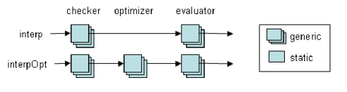
During this phase, we have to not only identify components but also define interfaces between components:

$$\begin{array}[]{lcccc}\mathsf{checker}&:&\mathsf{term}&\rightarrow&\mathsf{term}\\ \mathsf{optimizer}&:&\mathsf{term}&\rightarrow&\mathsf{term}\\ \mathsf{evaluator}&:&\mathsf{term}&\rightarrow&\mathsf{value}\end{array}$$

As usual, the arrow symbol $\rightarrow$ is used to specify a function type. In our example, components act like pipes in a pipe-and-filter architecture style, so all interface information is captured by the type. By using the above components, we can specify the overall structure of various interpreters:

$$\begin{array}[]{lcl}\mathsf{interp}&=&\mathsf{evaluator}~{}~{}\mathsf{o}~{}~{}\mathsf{checker}\\ \mathsf{interpOpt}&=&\mathsf{evaluator}~{}~{}\mathsf{o}~{}~{}\mathsf{optimizer}~{}~{}\mathsf{o}~{}~{}\mathsf{checker}\end{array}$$

5.3.3 Product line component design

Next, we identify conceptual components which are constituents of a conceptual architecture. A conceptual component can have multiple implementations. For example, there are many versions of the $\mathsf{evaluator}$ component depending on the evaluation strategy:

$$\begin{array}[]{lcccc}\mathsf{eval}&:&\mathsf{term}&\rightarrow&\mathsf{value}\\ \mathsf{eval}_{\mathsf{m}}&:&\mathsf{term}&\rightarrow&\mathsf{value}\end{array}$$

At the same time, the language $\mathsf{term}$ can be extended to become $\mathsf{term}^{\prime}$ which is an extension of $\mathsf{term}$ (for example to support conditionals):

$$\begin{array}[]{lcccc}\mathsf{eval}^{\prime}&:&\mathsf{term}^{\prime}&\rightarrow&\mathsf{value}\\ \mathsf{eval}^{\prime}_{\mathsf{m}}&:&\mathsf{term}^{\prime}&\rightarrow&\mathsf{value}\end{array}$$

Similarly, $\mathsf{check}$ and $\mathsf{check}^{\prime}$ can be specified as follows:

$$\begin{array}[]{lcccc}\mathsf{check}&:&\mathsf{term}&\rightarrow&\mathsf{term}\\ \mathsf{check}^{\prime}&:&\mathsf{term}^{\prime}&\rightarrow&\mathsf{term}^{\prime}\end{array}$$

For the $\mathsf{optimizer}$ component, there are many possible variations due to inclusion or exclusion of various individual optimization steps (here: constant folding and short-circuiting) and due to the variations in the underlying term language (here: basic and extended):

$$\begin{array}[]{lcccc}\mathsf{opt}_{\mathsf{cons}}&:&\mathsf{term}&\rightarrow&\mathsf{term}\\ \mathsf{opt}^{\prime}_{\mathsf{cons}}&:&\mathsf{term}^{\prime}&\rightarrow&\mathsf{term}^{\prime}\\ \mathsf{opt}^{\prime}_{\mathsf{short}}&:&\mathsf{term}^{\prime}&\rightarrow&\mathsf{term}^{\prime}\\ \mathsf{opt}^{\prime}_{\mathsf{cons+short}}&:&\mathsf{term}^{\prime}&\rightarrow&\mathsf{term}^{\prime}\end{array}$$

5.3.4 Product analysis

Product engineering starts with analyzing the requirements provided by the user and finds a corresponding set of required features from the feature model. Assuming we are to build four kinds of interpreters, we have to have four different feature selections:

$$\begin{array}[]{lcl}\mathsf{FS}(\mathsf{I})&=&\{\mathsf{Evaluation~{}semantics}\}\\ \mathsf{FS}(\mathsf{I}_{\mathsf{m}})&=&\{\mathsf{Machine~{}semantics}\}\\ \mathsf{FS}(\mathsf{I}_{\mathsf{opt}})&=&\{\mathsf{Machine~{}semantics,Optimizer,Constant~{}folding}\}\\ \mathsf{FS}(\mathsf{I}^{\prime}_{\mathsf{opt}})&=&\{\mathsf{Conditional,Evaluation~{}semantics,Optimizer,Constant~{}folding,Short-circuit}\}\end{array}$$

Here, the function $\mathsf{FS}$ maps a feature product to its corresponding set of its required features. (For brevity only non-mandatory features are shown.)

During product engineering, these selected feature sets give advice on the selection among both reference architectures and components. Figure 5.4 shows the overall product engineering process where the reference architecture $\mathsf{interpOpt}$ gets selected, guided by the presence of the $\mathsf{Optimizer}$ feature. Feature sets also show which components need to be selected and how they would be instantiated at the component level. For example, the presence of the $\mathsf{Constant~{}folding}$ feature guides us to choose the component $\mathsf{optimizer}$ with the implementation $\mathsf{opt_{cons}}$. Similarly, the presence of the $\mathsf{Machine~{}semantics}$ feature picks the implementation $\mathsf{eval_{m}}$ instead of $\mathsf{eval}$. The target product would be instantiated by assembling such selections.

Refer to caption
Figure 5.4: Product engineering.

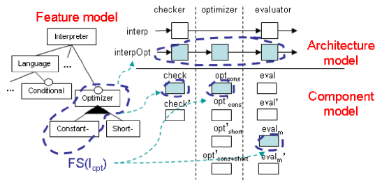
5.4 Issues in product line implementation

During the product line asset development process, we obtain reference models which represent architectural and component-level variations. Such variations should be realized at the code level. The first step is to refine conceptual architectures into concrete architectures which describe how to configure conceptual components. Then, product line component design involves realization of conceptual components using the proper product feature delivery methods. This section discusses some issues that surface during product line implementation.

Product line architecture implementation

In order to specify concrete reference architectures, we have to not only identify conceptual components but also define interfaces between components. Moreover, since there may be multiple reference architectures, it would be convenient to have mechanisms for abstracting architectural variations, capturing the inclusion or exclusion of certain components. Therefore, any adequate implementation technique should be able to provide mechanisms for:

  • Declaration of required conceptual components ($\mathsf{checker}$, $\mathsf{optimizer}$ and $\mathsf{evaluator}$) and their interfaces,

  • Specification of the base reference architecture $\mathsf{interp}$ and its optimized counterparts $\mathsf{interpOpt}$ by using such conceptual components.

Product line component implementation.

This phase involves realization of conceptual components. The main challenge of this phase is in how to implement generic components that encapsulate component-level variations. Such variations could be in the form of either code extension or code substitution. Any solution to the traditional expression problem can be a mechanism to implement code extension. For our running example, the following pairs correspond to code extension:

  • $\mathsf{check}$ and $\mathsf{check}^{\prime}$

  • $\mathsf{eval}$ and $\mathsf{eval}^{\prime}$

  • $\mathsf{eval}_{\mathsf{m}}$ and $\mathsf{eval}^{\prime}_{\mathsf{m}}$

  • $\mathsf{opt_{cons}}$ and $\mathsf{opt^{\prime}_{cons}}$

  • $\mathsf{opt}_{\mathsf{cons}}$ and $\mathsf{opt}^{\prime}_{\mathsf{cons+short}}$

  • $\mathsf{opt}^{\prime}_{\mathsf{short}}$ and $\mathsf{opt}^{\prime}_{\mathsf{cons+short}}$

Code substitution provides another form of variation at the component level when two different implementations provide interchangeable functionality. For example, $\mathsf{eval}$ and $\mathsf{eval_{m}}$ both implement the $\mathsf{evaluator}$ component, but neither is an extension of the other. Language abstraction mechanisms are expected to handle this case elegantly. For our running example, the corresponding scenarios are as follows:

  • $\mathsf{eval}$ and $\mathsf{eval}_{\mathsf{m}}$

  • $\mathsf{eval}^{\prime}$ and $\mathsf{eval}^{\prime}_{\mathsf{m}}$

Product engineering

Based on the product analysis, a feature product is instantiated by assembling product line core assets. For our running example, the evaluated techniques should be able to instantiate four interpreters ($\mathsf{I},\mathsf{I_{m}},\mathsf{I_{opt}},\mathsf{I^{\prime}_{opt}}$) based on the selected feature set.

5.5 Language supports for product line implementation

In this section, we illustrate how the MLPolyR language can be used to implement a two-way extensible interpreter. First, we show how each issue identified in the previous chapter will be resolved by various mechanisms provided by MLPolyR. A comparison with other product line implementation techniques follows.

Product line architecture implementation

Each component in a reference architecture is mapped to an MLPolyR module. As specified in Section 5.4, we first define types (or signatures) of the interested components based on the outcome of product line architecture design. (Section 5.3.2):

$$\begin{array}[]{lclccll}\mathsf{Checker}&:&\{\{&\mathsf{check}&:&\mathsf{term}\rightarrow\mathsf{term},&\ldots~{}\}\}\\ \mathsf{Optimizer}&:&\{\{&\mathsf{opt}&:&\mathsf{term}\rightarrow\mathsf{term},&\ldots~{}\}\}\\ \mathsf{Evaluator}&:&\{\{&\mathsf{eval}&:&\mathsf{term}\rightarrow\mathsf{int},&\ldots~{}\}\}\end{array}$$

where $\ldots$ indicates that there may be more parts in a component, but they are not our concerns. In practice, we do not have to write such interfaces explicitly since the type checker infers the principal types. Then, by using these conceptual modules ($\mathsf{Checker}$, $\mathsf{Optimizer}$ and $\mathsf{Evaluator}$), we can define two reference architectures:

module Interp = {{
val interp = fn e => Evaluator.eval(Check.check e)
}}
module InterpOpt = {{
val interp = fn e => Evaluator.eval(Optimizer.opt(Checker.check e))
}}

Alternatively, like functors in SML, we can use a parameterization technique called a template which takes concrete modules as arguments and instantiates a composite module:

template InterpFun (C, E) = {{
val interp = fn e => E.eval (C.check e)
}}
template InterpOptFun (C, O, E) = {{
val interp = fn e => E.eval (O.opt (C.check e))
}}

where $\mathsf{C}$, $\mathsf{O}$ and $\mathsf{E}$ represent $\mathsf{Checker}$, $\mathsf{Optimizer}$ and $\mathsf{Evaluator}$ respectively. Their signatures are captured as constraints by the type checker. For example, the type checker infers the constraint that the module $\mathsf{C}$ should have a component named $\mathsf{check}$ which has a type of $\alpha\rightarrow\beta$ and $\beta$ should be either an argument type of the module $\mathsf{E}$ (Line 1) or that of $\mathsf{O}$ (Line 5).

The second approach with templates supports more code reuse because a reference architecture becomes polymorphic, i.e., parameterized not only over the values but also over the types of its components. As long as components satisfy constraints that the type checker computes, any components can be plugged into a reference architecture. For example, for the argument $\mathsf{C}$, either the base module $\mathsf{Check}$ and its extension $\mathsf{EChecker}$ can applied to the template $\mathsf{InterpFun}$.

Product line component implementation

Modules in MLPolyR implement components. In order to manage component-level variations, we have to deal with both code extension and code substitution as discussed in Section 5.4. For example, we will see multiple implementations of the component $\mathsf{Evaluator}$:

$$\begin{array}[]{lclccll}\mathsf{BigStep}&:&\{\{&\mathsf{eval}&:&\mathsf{term}\rightarrow\mathsf{int},&\ldots~{}\}\}\\ \mathsf{Machine}&:&\{\{&\mathsf{eval}&:&\mathsf{term}\rightarrow\mathsf{int},&\ldots~{}\}\}\\ \mathsf{EBigStep}&:&\{\{&\mathsf{eval}&:&\mathsf{term}^{\prime}\rightarrow\mathsf{int},&\ldots~{}\}\}\\ \mathsf{EMachine}&:&\{\{&\mathsf{eval}&:&\mathsf{term}^{\prime}\rightarrow\mathsf{int},&\ldots~{}\}\}\par\end{array}$$

where $\mathsf{term}$ represents a type of the base constructors and $\mathsf{term}^{\prime}$ that of the extension. $\mathsf{BigStep}$ and $\mathsf{EBigStep}$ implement the evaluation semantics and its extension while $\mathsf{Machine}$ and $\mathsf{EMachine}$ implement the machine semantics and its extension. Note that the pair of $\mathsf{BigStep}$ and $\mathsf{EBigStep}$ and also the pair of $\mathsf{Machine}$ and $\mathsf{EMachine}$ correspond to code extension while the pair of $\mathsf{BigStep}$ and $\mathsf{Machine}$ corresponds to code substitution.

Code extension is supported by first-class extensible cases as we already studied in Section 3.2. Figure 5.5 shows how such extensions are made. In an extension, only a new case is handled (Line 19-21) and the default explicitly refers to the original set of other cases represented by $\mathsf{BigStep.bases}$ (Line 22).

(* module for the evaluation semantics *)
module BigStep = {{
fun bases (eval, env) =
cases VAR x => env x
| NUM n => n
| PLUS (e1, e2) => eval (env, e1) + eval (env, e2)
| LET (x, e1, e2) =>
eval (Envt.bind (eval (env, e1), x, env), e2)
fun eval e =
let fun run (env, e) = match e with bases (run, env)
in run (Envt.empty, e)
end
}}
(* module for the extended evaluation semantics *)
module EBigStep = {{
fun bases (eval, env) =
cases IF0 (e1, e2, e3) =>
if eval (env, e1) == 0 then eval (env, e2)
else eval (env, e3)
default: BigStep.bases (eval, env)
fun eval e =
let fun run (env, e) = match e with bases (run, env)
in run (Envt.empty, e)
end
}}
Figure 5.5: The module $\mathsf{BigStep}$ realizes the evaluation semantics ($\mathsf{eval}$), and the module $\mathsf{EBigStep}$ realizes the extended evaluation semantics ($\mathsf{eval^{\prime}}$) by defining only a new case $\mathsf{`IF0}$. In an extension, only a new case is handled (Line 19-21) and the default explicitly refers to the original set of other cases represented by $\mathsf{BigStep.bases}$ (Line 22). Then, $\mathsf{EBigStep.bases}$ can handle five cases including $\mathsf{IF0}$. We can obtain a new evaluator $\mathsf{EBigStep.eval}$ by closing the recursion through applying $\mathsf{bases}$ to evaluator itself (Line 25). Note that a helper function $\mathsf{run}$ is actually applied instead of $\mathsf{eval}$ in order to pass an initial environment in Line 26.
(* module for the machine semantics *)
module Machine = {{
fun ecases (K, env, estate, vstate) =
cases VAR x => env x
| NUM n => vstate (n, K)
| PLUS (e1, e2) => estate (‘PLUSl (e2, env)::K, env, e1)
| LET (x, e1, e2) => estate (‘LETl (x, e2, env)::K, env, e1)
and vcases (v, K, estate, vstate) =
cases PLUSl (e, env) => estate((‘PLUSr v)::K, env, e)
| LETl (x, e, env) => estate (K, Envt.bind (v, x, env), e)
| PLUSr v => vstate (v’+v, K)
fun estate (K, env, e) = match e with ecases (K, env, estate, vstate)
and vstate (v, K) =
case K of
[] => v
| h::tl => match h with vcases (v, tl, estate, vstate)
fun eval e = estate ([], Envt.empty, e)
}}
(* module for the extended machine semantics *)
module EMachine = {{
fun ecases (K, env, estate, vstate) =
cases IF0 (e1, e2, e3) =>
estate (‘IF0l (e2, e3, env)::K, env, e1)
default: Machine.ecases (K, env, estate, vstate)
and vcases (v, K, estate, vstate) =
cases IF0l (e2, e3, env) =>
if v == 0 then estate (K, env, e2) else estate (K, env, e3)
default: Machine.vcases (v, K, estate, vstate)
fun estate (K, env, e) = match e with ecases (K, env, estate, vstate)
and vstate (v, K) =
case K of
[] => v
| h::tl => match h with vcases (v, tl, estate, vstate)
fun eval e = estate ([], Envt.empty, e)
}}
Figure 5.6: The module $\mathsf{Machine}$ realizes the machine semantics ($\mathsf{eval_{m}}$), and the module $\mathsf{EMachine}$ realizes the extended machine semantics ($\mathsf{eval^{\prime}_{m}}$) by defining only new cases $\mathsf{`IF0}$ and $\mathsf{`IF0l}$.

Code substitution as another form of variation at the component level does not cause any trouble. For example, Figure 5.6 shows the module $\mathsf{Machine}$ which implements the machine semantics (i.e., $\mathsf{eval_{m}}$). Like $\mathsf{BigStep}$ and $\mathsf{EBigStep}$, $\mathsf{EMachine}$ extends $\mathsf{Machine}$ through two extensible cases (Line 27 and 31). In our example two different implementations ($\mathsf{BigStep}$ and $\mathsf{Machine}$) provide interchangeable functionality, but neither is an extension of the other, so they are implemented independently.

Analogously, we can implement the remaining two conceptual components $\mathsf{Checker}$ and $\mathsf{Optimizer}$. For $\mathsf{Checker}$ we have,

$$\begin{array}[]{lclccll}\mathsf{Check}&:&\{\{&\mathsf{check}&:&\mathsf{term}\rightarrow\mathsf{term},&\ldots~{}\}\}\\ \mathsf{ECheck}&:&\{\{&\mathsf{check}&:&\mathsf{term}^{\prime}\rightarrow\mathsf{term}^{\prime},&\ldots~{}\}\}\end{array}$$

where each implements the concrete component $\mathsf{check}$ and $\mathsf{check^{\prime}}$, respectively. For the component $\mathsf{Optimizer}$,

$$\begin{array}[]{lclccll}\mathsf{COptimizer}&:&\{\{&\mathsf{opt}&:&\mathsf{term}\rightarrow\mathsf{term},&\ldots~{}\}\}\\ \mathsf{ECOptimizer}&:&\{\{&\mathsf{opt}&:&\mathsf{term}^{\prime}\rightarrow\mathsf{term}^{\prime},&\ldots~{}\}\}\\ \mathsf{ESOptimizer}&:&\{\{&\mathsf{opt}&:&\mathsf{term}^{\prime}\rightarrow\mathsf{term}^{\prime},&\ldots~{}\}\}\\ \mathsf{ECSOptimizer}&:&\{\{&\mathsf{opt}&:&\mathsf{term}^{\prime}\rightarrow\mathsf{term}^{\prime},&\ldots~{}\}\}\end{array}$$

where each implements the concrete component $\mathsf{opt_{cons}}$, $\mathsf{opt^{\prime}_{cons}}$, $\mathsf{opt^{\prime}_{short}}$ and $\mathsf{opt^{\prime}_{cons+short}}$, respectively.

Product engineering

In Section 5.3.4, we define four interpreters ($\mathsf{I}$, $\mathsf{I_{m}}$, $\mathsf{I_{opt}}$, and $\mathsf{I^{\prime}_{opt}}$) differentiated by the feature selection. Each will be instantiated by selecting a proper architecture (either $\mathsf{InterpFun}$ and $\mathsf{InterOptFun}$) and choosing its components (either $\mathsf{BigStep}$ or $\mathsf{Machine}$, etc) with implicit advice from the selected feature set. For example:

  • When the feature set is $\mathsf{FS(I)}$, the reference architecture $\mathsf{InterpFun}$ gets selected since the $\mathsf{Optimizer}$ feature is not in the set. Then, the proper components are selected and instantiated. For example, the presence of the $\mathsf{Evaluation~{}semantics}$ feature guides us to choose the component $\mathsf{BigStep}$ instead of $\mathsf{Machine}$. Therefore, we instantiate the interpreter $\mathsf{I}$ as follows:

    $$\begin{array}[]{@{}l@{~~}c@{~~}ll}\mathsf{module~{}I}\hfil~{}~{}&=\hfil~{}~{}&\mathsf{InterpFun}&(\mathsf{Checker},\mathsf{BigStep})\end{array}$$
  • When the feature set is $\mathsf{FS(I_{m})}$, the reference architecture $\mathsf{InterpFun}$ gets chosen. Here, components $\mathsf{Machine}$ and $\mathsf{Check}$ are selected because of the presence of $\mathsf{Machine~{}semantics}$ feature. Therefore, we instantiate the interpreter $\mathsf{I_{m}}$ as follows:

    $$\begin{array}[]{@{}l@{~~}c@{~~}ll}\mathsf{module~{}I_{m}}\hfil~{}~{}&=\hfil~{}~{}&\mathsf{InterpFun}&(\mathsf{Checker},\mathsf{Machine})\end{array}$$
  • When the feature set is $\mathsf{FS(I_{opt})}$, the reference architecture $\mathsf{InterpOptFun}$ is chosen since the $\mathsf{Optimizer}$ feature is in the set. Then, again, the proper components get selected and instantiated. Here, the presence of the $\mathsf{Constant~{}folding}$ feature guides us to choose the component $\mathsf{COptimizer}$ and the presence of the $\mathsf{Machine~{}semantics}$ feature leads us to instantiate the component $\mathsf{Machine}$. Therefore, we instantiate the interpreter $\mathsf{I_{opt}}$ as follows:

    $$\begin{array}[]{@{}l@{~~}c@{~~}ll}\mathsf{module~{}I_{opt}}\hfil~{}~{}&=\hfil~{}~{}&\mathsf{InterpOptFun}&(\mathsf{Checker},\\ \hfil~{}~{}&\hfil~{}~{}&&~{}~{}\mathsf{COptimizer},\\ \hfil~{}~{}&\hfil~{}~{}&&~{}~{}\mathsf{Machine})\end{array}$$
  • When the feature set is $\mathsf{FS(I^{\prime}_{opt})}$, the reference architecture $\mathsf{InterpOptFun}$ is chosen. As far as the components are concerned, the presence of the $\mathsf{Conditional}$ and $\mathsf{Evaluation~{}semantics}$ features guide us to choose the component $\mathsf{EBigStep}$. Similarly, the presence of the $\mathsf{Optimizer}$, $\mathsf{Conditional}$, $\mathsf{Constant~{}folding}$ and $\mathsf{Short-circuit}$ forces the use of component $\mathsf{ECSOptimizer}$. Therefore, we instantiate the interpreter $\mathsf{I^{\prime}_{opt}}$ as follows:

    $$\begin{array}[]{@{}l@{~~}c@{~~}ll}\mathsf{module~{}I^{\prime}_{opt}}\hfil~{}~{}&=\hfil~{}~{}&\mathsf{InterpOptFun}&(\mathsf{EChecker},\\ \hfil~{}~{}&\hfil~{}~{}&&~{}~{}\mathsf{ECSOptimizer},\\ \hfil~{}~{}&\hfil~{}~{}&&~{}~{}\mathsf{EBigStep})\end{array}$$

5.6 Evaluation

Although they are not intended to aim specifically for feature-oriented programming, many language constructs can be used to manage variability in the context of product line implementation. For example, various mechanisms including classes, aspects and modules can support abstraction of features. They also support extension mechanisms such as sub-classing, macro processing, aspect-weaving or parameterizing, which can be used to modularize feature composition. Among various techniques, there are three representative implementation approaches which can be found frequently in the product line literature (Gacek and Anastasopoules 2001; Kästner et al. 2008).

The annotative approach

As the name suggests, the annotative approaches implement features using some form of annotations. Typically, preprocessors, e.g., macro systems, have been used in many literature examples as the feature product delivery method (Kang et al. 1998, 2005). For example, the macro language in FORM determines inclusion or exclusion of some code segments based on the feature selection:

val interp =
fn e => Evaluator.eval
$IF(;:$Optimizer) [
(Optimizer.opt
(Check.check e))
][
(Check.check e)
]

Depending on the presence of the $\mathsf{Optimizer}$ feature, either block (4-5 or 7) will be selected.

Macro languages have some advantage in that they can be mixed easily with any target programming languages. However, feature specific segments are scattered across multiple classes, so code easily becomes complicated. Saleh and Gomaa propose the feature description language (Saleh and Gomaa 2005). Its syntax looks similar to the C/C++ preprocessor but it supports separation of concerns by modularizing feature specific code in a separate file. In the annotation approach, however, target compilers do not understand the macro language and any error appearing in feature code segments cannot be detected until all feature sets are selected and the corresponding code segments are compiled.

The compositional approach

For taking advantage of the current compiler technology including static typing and separate compilation, we need native language supports. Therefore, language-oriented proposals generally take compositional approaches by providing better support for feature modularity (Lopez-Herrejon et al. 2005). FeatureC++ (Apel et al. 2005), AHEAD (Batory 2004) and AspectJ are such language extensions.

In this approach, features are implemented as distinct units and then they are combined to become a product. Aspect-oriented programming has become popular as a way of implementing the compositional approach (Lee et al. 2006; Cho et al. 2008). The main idea is to implement variations as separate aspects and to obtain each product by weaving base code and aspect code. Our extensible cases provide similar composability. Furthermore, our module language also supports extensible modules, which make large-scale code reusable. Note that composition in aspects does not provide separate compilation, so base code requires to be either re-typed-checked or re-compiled or both for every composition. However, our module system supports separate compilation.

The parameterization approach

The idea of parameterized programming is to implement the common part once and parameterize variations so that different products can be instantiated by assigning distinct values as parameters. Functors, as provided by Standard ML (SML), are a typical example in that they can be parameterized on values, types and other modules (Appel and MacQueen 1991). The SML module system has been demonstrated to be powerful enough to manage variations in the context of product lines (Chae and Blume 2008). However, its type system sometimes imposes restrictions which require code duplication between functions on data types. Many proposals to overcome this restriction have been presented. For example, MLPolyR proposes extensible cases (Blume et al. 2006), and OCaml proposes polymorphic variants (Garrigue 2000).

Similarly, templates in C++ provide parameterization over types and have been extensively studied in the context of programming families  (Czarnecki and Eisenecker 2000). Recently, an improvement that would provide better support of generic programming has been proposed (Dos Reis and Stroustrup 2006). Originally, Java and C# did not support parameterized types but now both support similar concepts (Torgersen 2004).

Sometimes the parameterization approach is criticized for its difficulty in identifying variation points and defining parameters (Gacek and Anastasopoules 2001). However, systematic reasoning (e.g., product line analysis done by product line architects) can ease such burden by providing essential information for product line implementation  (Chae and Blume 2008).

Chapter 6 Conclusion

Software evolves by means of change. Changes may be implemented either sequentially or in parallel. Sequential changes form a series of software releases. Some changes carried out in parallel may also be merged back together. In this situation, we are interested in extension mechanisms which provide a way to add extensions in a reliable way. Some changes implemented in parallel, however, cannot be combined together so a single software product diverges into different versions. In this case, multiple software versions may evolve independently although much of their code is duplicated, which makes it difficult to maintain them. Under these circumstances, we need a way of managing variability among multiple versions so that we can easily manage the evolution of a set of products.

In this thesis, we propose type-safe extensible programming which takes two dimensions into consideration. In particular, our language provides type-safe extensibility mechanisms at multiple levels of granularity, from the fine degree (at the core expression level) to the coarse degree (at the module level). At the same time, in order to manage variability, we adopt product line engineering as a developing paradigm and then show how our extensibility mechanisms can be used to implement a set of products:

  • In Section 3, we propose a core language that supports polymorphic extensible records, first-class cases and type safe exception handling. With cases being first-class and extensible, we show that our language enables a very flexible style of composable extension;

  • In Section 4, we propose a module system that makes extensible programming at the module level possible. We also show how to compile each module separately in the presence of all of the above features;

  • In Section 5, we propose a development process which adopts product line engineering in order to manage variability in a family of systems. We show that our extensibility mechanisms can be put to good use in the context of product line implementation.

We are continuing this work in several ways. First, we plan to improve our type system. For example, we have constructed a prototype compiler for MLPolyR that retains all of the MLPolyR features as well as mutable record fields. Records with mutable fields have identity, and allocation of such a record is a side-effecting operation. However, mutable data type can weaken our polymorphic type system, in situations where the so-called value restriction prevents row type variables from being generalized (Pessaux and Leroy 1999). Pessaux and Leroy presents such an example that shows a false positive:

let val r = {| i = fn x => x+1 |}
fun f y c = if c then r!i y
else raise Error ()
in r!i 0
end

First, $r$ has type $\mathbf{\{}{|i:\mathsf{int}\stackrel{{\scriptstyle\rho}}{{\rightarrow}}\mathsf{int}|}\mathbf{\}}$ where $\rho$ is not generalized since the whole expression is not a syntactic value (Line 1). Then, during typing $f$, a true branch with $r!i~{}y$ (Line 2) is unified with a false branch with $\mathbf{raise}~{}`\mathsf{Error}()$ (Line 3). Therefore, $\rho$ becomes $\mathsf{Error()};\rho^{\prime}$ and the application $r!i~{}0$ falsely appears to raise $\mathsf{Error()}$ even though it does not (Line 4). Pessaux and Leroy suggests that this false positive could be avoided with a more precise tracking of the flow of exceptions.

Additionally, as we discussed in Section 4.3, non-generalized unification variables in the presence of mutable references makes our type system unsound unless they are instantiated consistently across the module boundary. We plan to add a consistency checking mechanism during linking time.

Second, our module system does not require any type decoration since the type system infers module signatures as it infers types of core expressions. However, there will be a need for programmers to spell out types. For example, module signatures in libraries are generally required to be explicit. We plan to support explicit specification of module signatures and conventional signature matching as in SML. However, there can be situations where row types and kind information make it difficult to specify full typing information. As we have seen in Section 4.3, we might ask programmers to write the following type decoration for $\mathsf{map}$:

val map : $\forall\alpha:\star.\forall\beta:\star.\forall\gamma:\varnothing.\forall\delta:\varnothing.(\alpha\stackrel{{\scriptstyle\gamma}}{{\rightarrow}}\beta)\stackrel{{\scriptstyle\delta}}{{\rightarrow}}([\alpha]\stackrel{{\scriptstyle\gamma}}{{\rightarrow}}[\beta])$

It is possible to avoid this excessive notational overhead by defining a little language with good built-in defaults (e.g., abbreviation for common patterns). Then, programmers would specify their intentions using this language and these intended types can be checked against inferred types in a style of software contract  (Findler and Felleisen 2002; Blume and McAllester 2006). For example, we may specify $\mathsf{map}$’s type as follows and all elided parts can be inferred and checked by a compiler:

val map : $(\alpha\stackrel{{\scriptstyle\gamma}}{{\rightarrow}}\beta)\stackrel{{\scriptstyle}}{{\rightarrow}}([\alpha]\stackrel{{\scriptstyle\gamma}}{{\rightarrow}}[\beta])$

Third, we plan to integrate feature composition with our language. Our work shows that modern programming language technology such as extensible cases and parameterized modules is powerful enough to manage variability identified by product line analysis. However, in our approach, the relations among features, architectures, and components are implicitly expressed only during the product line analysis. Similarly, Most feature-oriented programming languages do not have the notion of a “feature” in the language syntax since features are merely considered conceptual abstractions rather than concrete language constructs. Therefore, these languages cannot state the relations between a feature and its corresponding code segments in the program text (Apel et al. 2008). However, other product line model-based methods usually provide a way to express those relations explicitly by using CASE tools. In FORM, for example, those explicit relations make it possible to automatically generate product code from specifications  (Kang et al. 1998).

In our recent work, we are proposing a macro system for MLPolyR, which augments the language with an explicit notion of features (Chae and Blume 2009). We implemented this mechanism in order to make it possible to write feature composition in terms of features. Then, the compiler can integrate the corresponding code automatically once we provide a valid feature set. Since our expansion rules do not support any specification of feature relationships (i.e., mutually exclusive or required relations), however, the MLPolyR compiler cannot detect any invalid feature sets. We leave such validation to feature modeling tools which provide various diagnoses on feature models. Our goal is to let a front-end modeling tool generate valid expansion rules in the MLPolyR language so that an application can automatically be assembled only by feature selection.

References

  • Apel et al. [2005] Sven Apel, Thomas Leich, Marko Rosenmüller, and Gunter Saake. Featurec++: On the symbiosis of feature-oriented and aspect-oriented programming. In In Proceedings of the International Conference on Generative Programming and Component Engineering, pages 125–140. Springer, 2005.
  • Apel et al. [2008] Sven Apel, Christian Kästner, and Christian Lengauer. Feature featherweight java: a calculus for feature-oriented programming and stepwise refinement. In GPCE ’08: Proceedings of the 7th international conference on Generative programming and component engineering, pages 101–112, New York, NY, USA, 2008. ACM. ISBN 978-1-60558-267-2.
  • Appel [1994] Andrew Appel. Hot-sliding in ML, 1994.
  • Appel [1992] Andrew W. Appel. Compiling with Continuations. Cambridge University Press, Cambridge, England, 1992.
  • Appel and MacQueen [1991] Andrew W. Appel and David B. MacQueen. Standard ML of New Jersey. In Martin Wirsing, editor, 3rd International Symp. on Prog. Lang. Implementation and Logic Programming, pages 1–13, New York, August 1991. Springer-Verlag.
  • Armstrong [2007] Joe Armstrong. Programming Erlang: Software for a Concurrent World. Pragmatic Bookshelf, July 2007. ISBN 193435600X.
  • AspectJ [2008] AspectJ. http://www.eclipse.org/aspectj/, 2008.
  • Batory [2004] Don Batory. Feature-oriented programming and the ahead tool suite. In ICSE ’04: Proceedings of the 26th International Conference on Software Engineering, pages 702–703, Washington, DC, USA, 2004. IEEE Computer Society. ISBN 0-7695-2163-0.
  • Blume and McAllester [2006] Matthias Blume and David McAllester. Sound and complete models of contracts. J. Funct. Program., 16(4-5):375–414, 2006. ISSN 0956-7968. http://dx.doi.org/10.1017/S0956796806005971.
  • Blume et al. [2006] Matthias Blume, Umut A. Acar, and Wonseok Chae. Extensible programming with first-class cases. In John H. Reppy and Julia L. Lawall, editors, ICFP, pages 239–250. ACM, 2006. ISBN 1-59593-309-3.
  • Blume et al. [2008] Matthias Blume, Umut A. Acar, and Wonseok Chae. Exception handlers as extensible cases. In the Sixth ASIAN Symposium on Programming Languages and Systems (APLAS 2008), December 2008.
  • Bourdoncle and Merz [1997] François Bourdoncle and Stephan Merz. Type-checking higher-order polymorphic multi-methods. In Conference Record of POPL ’97: The 24th ACM SIGPLAN-SIGACT Symposium on Principles of Programming Languages, pages 302–315, Paris, France, 15–17 1997. URL citeseer.ist.psu.edu/bourdoncle97type.html.
  • Bruce [2003] Kim B. Bruce. Some challenging typing issues in object-oriented languages. In Electronic notes in Theoretical Computer Science, volume 82(8), 2003. URL citeseer.ist.psu.edu/bruce03some.html.
  • Buckley et al. [2005] Jim Buckley, Tom Mens, Matthias Zenger, Awais Rashid, and Günter Kniesel. Towards a taxonomy of software change: Research articles. J. Softw. Maint. Evol., 17(5):309–332, 2005. ISSN 1532-060X. http://dx.doi.org/10.1002/smr.v17:5.
  • Chae and Blume [2008] Wonseok Chae and Matthias Blume. Building a family of compilers. In SPLC ’08: Proceedings of the 12th International Software Product Line Conference, Limerick, Ireland, 2008. IEEE Computer Society. ISBN 0-7695-2888-0.
  • Chae and Blume [2009] Wonseok Chae and Matthias Blume. Language Support for Feature-Oriented Product Line Engineering. In FOSD’09: Proceedings of the first International Workshop on Feature-Oriented Software Development, Denver, Colorado, 2009.
  • Cho et al. [2008] Hojin Cho, Kwanwoo Lee, and Kyo C. Kang. Feature relation and dependency management: An aspect-oriented approach. Software Product Line Conference, International, 0:3–11, 2008. http://doi.ieeecomputersociety.org/10.1109/SPLC.2008.23.
  • Czarnecki [2004] Krzysztof Czarnecki. Generative software development. In SPLC, page 321, 2004.
  • Czarnecki and Eisenecker [2000] Krzysztof Czarnecki and Ulrich W. Eisenecker. Generative programming: methods, tools, and applications. ACM Press/Addison-Wesley Publishing Co., New York, NY, USA, 2000. ISBN 0-201-30977-7.
  • Dos Reis and Stroustrup [2006] Gabriel Dos Reis and Bjarne Stroustrup. Specifying c++ concepts. In POPL ’06: Conference record of the 33rd ACM SIGPLAN-SIGACT symposium on Principles of programming languages, pages 295–308, New York, NY, USA, 2006. ACM. ISBN 1-59593-027-2. http://doi.acm.org/10.1145/1111037.1111064.
  • Dreyer and Blume [2006] Derek Dreyer and Matthias Blume. Principal type schemes for modular programs. In European Symposium on Programming (ESOP), 2006.
  • Elsman [2008] Martin Elsman. A framework for cut-off incremental recompilation and inter-module optimization. IT University of Copenhagen, Denmark. IT University Technical Report, 2008.
  • Felleisen and Hieb [1992] Matthias Felleisen and Robert Hieb. A revised report on the syntactic theories of sequential control and state. Theoretical Computer Science, 103(2):235–271, 1992. URL citeseer.nj.nec.com/felleisen92revised.html.
  • Findler and Felleisen [2002] Robert Bruce Findler and Matthias Felleisen. Contracts for higher-order functions. SIGPLAN Not., 37(9):48–59, 2002. ISSN 0362-1340. http://doi.acm.org/10.1145/583852.581484.
  • Findler and Flatt [1999] Robert Bruce Findler and Matthew Flatt. Modular object-oriented programming with units and mixins. In ICFP ’99: Proceedings of the fourth ACM SIGPLAN international conference on Functional programming, volume 34(1) of SIGPLAN, pages 94–104, New York, NY, June 1999. ACM.
  • Flanagan et al. [1993] Cormac Flanagan, Amr Sabry, Bruce F. Duba, and Matthias Felleisen. The Essence of Compiling with Continuations. In 1993 Conference on Programming Language Design and Implementation., pages 21–25, June 1993.
  • Flatt [1999] Matthew Flatt. Programming Languages for Reusable Software Components. PhD thesis, Department of Computer Science, Rice University, 1999. URL overcite.lcs.mit.edu/flatt99programming.html.
  • Gacek and Anastasopoules [2001] Critina Gacek and Michalis Anastasopoules. Implementing product line variabilities. SIGSOFT Softw. Eng. Notes, 26(3):109–117, 2001. ISSN 0163-5948. http://doi.acm.org/10.1145/379377.375269.
  • Gamma et al. [1995] Erich Gamma, Richard Helm, Ralph Johnson, and John Vlissides. Design patterns: elements of reusable object-oriented software. Addison-Wesley Professional, 1995.
  • Gansner and Reppy [2002] Emden R. Gansner and John H. Reppy. The Standard ML Basis Library. Cambridge University Press, New York, NY, USA, 2002. ISBN 0-52179-478-1.
  • Garcia et al. [2007] Ronald Garcia, Jaakko Jarvi, Andrew Lumsdaine, Jeremy Siek, and Jeremiah Willcock. An extended comparative study of language support for generic programming. J. Funct. Program., 17(2):145–205, 2007. ISSN 0956-7968. http://dx.doi.org/10.1017/S0956796806006198.
  • Garlan and Shaw [1994] David Garlan and Mary Shaw. An introduction to software architecture. Technical report, Carnegie Mellon University, Pittsburgh, PA, USA, 1994.
  • Garrigue [2000] Jacques Garrigue. Code reuse through polymorphic variants. In Workshop on Foundations of Software Engineering, November 2000.
  • Garrigue [1998] Jacques Garrigue. Programming with polymorphic variants. In ACM SIGPLAN Workshop on ML, 1998.
  • [35] GCC. The GNU Compiler Collection, http://gcc.gnu.org/.
  • Harper [2005] Robert Harper. Draft at http://www.cs.cmu.edu/~rwh/, 2005.
  • Jones et al. [1999] Simon Peyton Jones, Norman Ramsey, and Fermin Reig. C-: A portable assembly language that supports garbage collection, 1999.
  • Kang et al. [1998] Kyo C. Kang, Sajoong Kim, Jaejoon Lee, Kijoo Kim, Euiseob Shin, and Moonhang Huh. Form: A feature-oriented reuse method with domain-specific reference architectures. Ann. Softw. Eng., 5:143–168, 1998. ISSN 1022-7091.
  • Kang et al. [2002] Kyo C. Kang, Jaejoon Lee, and Patrick Donohoe. Feature-oriented product line engineering. IEEE Softw., 19(4):58–65, 2002. ISSN 0740-7459. http://dx.doi.org/10.1109/MS.2002.1020288.
  • Kang et al. [2005] Kyo Chul Kang, Moonzoo Kim, Jaejoon Lee, and Byungkil Kim. Feature-oriented re-engineering of legacy systems into product line assets - a case study. In SPLC, pages 45–56, 2005.
  • Kästner et al. [2008] Christian Kästner, Sven Apel, and Martin Kuhlemann. Granularity in software product lines. In ICSE ’08: Proceedings of the 30th international conference on Software engineering, pages 311–320, New York, NY, USA, 2008. ACM. ISBN 978-1-60558-079-1. http://doi.acm.org/10.1145/1368088.1368131.
  • Krishnamurthi et al. [1998] Shriram Krishnamurthi, Matthias Felleisen, and Daniel P. Friedman. Synthesizing Object-Oriented and Functional Design to Promote Re-Use. In European Conference on Object-Oriented Programming, 1998.
  • Lee et al. [2000] Kwanwoo Lee, Kyo C. Kang, Eunman Koh, Wonsuk Chae, Bokyoung Kim, and Byoung Wook Choi. Domain-oriented engineering of elevator control software: a product line practice. In Proceedings of the first conference on Software product lines : experience and research directions, pages 3–22, Norwell, MA, USA, 2000. Kluwer Academic Publishers. ISBN 0-79237-940-3.
  • Lee et al. [2002] Kwanwoo Lee, Kyo Chul Kang, and Jaejoon Lee. Concepts and guidelines of feature modeling for product line software engineering. In ICSR-7: Proceedings of the 7th International Conference on Software Reuse, pages 62–77, London, UK, 2002. Springer-Verlag. ISBN 3-540-43483-6.
  • Lee et al. [2006] Kwanwoo Lee, Kyo C. Kang, Minseong Kim, and Sooyong Park. Combining feature-oriented analysis and aspect-oriented programming for product line asset development. In SPLC ’06: Proceedings of the 10th International on Software Product Line Conference, pages 103–112, Washington, DC, USA, 2006. IEEE Computer Society. ISBN 0-7695-2599-7.
  • Leroy [2006] Xavier Leroy. Formal certification of a compiler back-end or: programming a compiler with a proof assistant. In POPL ’06: Conference record of the 33rd ACM SIGPLAN-SIGACT symposium on Principles of programming languages, pages 42–54, New York, NY, USA, 2006. ACM. ISBN 1-59593-027-2. http://doi.acm.org/10.1145/1111037.1111042.
  • Lopez-Herrejon et al. [2005] Roberto E. Lopez-Herrejon, Don Batory, and William Cook. Evaluating support for features in advanced modularization technologies. In ECOOP, pages 169–194. Springer, 2005.
  • Matzan [2007] Jem Matzan. More on OpenBSD’s new compiler. Available at http://www.thejemreport.com/content/view/369/, 2007.
  • Microsoft [2006] Microsoft. http://www.microsoft.com/presspass/press/2006/feb06/02-26WinVistaProductsPR.mspx, 2006.
  • Millstein et al. [2002] Todd Millstein, Colin Bleckner, and Craig Chambers. Modular typechecking for hierarchically extensible datatypes and functions. In ICFP ’02: Proceedings of the seventh ACM SIGPLAN international conference on Functional programming, pages 110–122, New York, NY, USA, 2002. ACM Press. ISBN 1-58113-487-8. http://doi.acm.org/10.1145/581478.581489.
  • Milner [1978a] Robin Milner. A theory of type polymorphism in programming. Journal of Computer and System Sciences, 13(3):348–375, 1978a.
  • Milner [1978b] Robin Milner. A theory of type polymorphism in programming. J. Comput. Syst. Sci., 17(3):348–375, 1978b.
  • Monteiro [2006] Miguel P. Monteiro. Using design patterns as indicators of refactoring opportunities (to aspects). In Position paper for the workshop on Linking Aspect Technology and Evolution revisited (LATEr) at AOSD 2006, 2006.
  • Noda and Kishi [2008] Natsuko Noda and Tomoji Kishi. Aspect-oriented modeling for variability management. In SPLC ’08: Proceedings of the 2008 12th International Software Product Line Conference, pages 213–222, Washington, DC, USA, 2008. IEEE Computer Society. ISBN 978-0-7695-3303-2. http://dx.doi.org/10.1109/SPLC.2008.44.
  • Norvig [1998] Peter Norvig. http://norvig.com/design-patterns, 1998.
  • Nystrom et al. [2003] Nathaniel Nystrom, Michael R. Clarkson, and Andrew C. Myers. Polyglot: An extensible compiler framework for java, 2003. URL citeseer.ist.psu.edu/nystrom03polyglot.html.
  • Odersky and Wadler [1997] Martin Odersky and Philip Wadler. Pizza into Java: Translating theory into practice. In Proceedings of the 24th ACM Symposium on Principles of Programming Languages (POPL’97), Paris, France, pages 146–159. ACM Press, New York (NY), USA, 1997. URL citeseer.ist.psu.edu/odersky97pizza.html.
  • Ohori and Yoshida [1999] Atsushi Ohori and Nobuaki Yoshida. Type inference with rank 1 polymorphism for type-directed compilation of ml. In ICFP ’99: Proceedings of the fourth ACM SIGPLAN international conference on Functional programming, pages 160–171, New York, NY, USA, 1999. ACM. ISBN 1-58113-111-9. http://doi.acm.org/10.1145/317636.317796.
  • Pessaux and Leroy [1999] François Pessaux and Xavier Leroy. Type-based analysis of uncaught exceptions. In POPL ’99: Proceedings of the 26th ACM SIGPLAN-SIGACT symposium on Principles of programming languages, pages 276–290, New York, NY, USA, 1999. ACM Press. ISBN 1-58113-095-3. http://doi.acm.org/10.1145/292540.292565.
  • Pierce [2002] Benjamin C. Pierce. Types and programming languages. MIT Press, Cambridge, MA, USA, 2002. ISBN 0-262-16209-1.
  • Rémy and Garrigue [2004] Didier Rémy and Jacques Garrigue. OCaml implementation of the ”Indepenently Extensible Solutions to the Expression Problem” code at http://pauillac.inria.fr/~remy/work/expre, 2004.
  • Rémy and Vouillon [1998] Didier Rémy and Jérôme Vouillon. Objective ML: An effective object-oriented extension to ML. Theory And Practice of Objects Systems, 4(1):27–50, 1998.
  • Reppy and Riecke [1996] John Reppy and Jon Riecke. Simple objects for Standard ML. In Proceedings of the ACM SIGPLAN ’96 Conference on Programming Language Design and Implementation, pages 171–180, Philadelphia, Pennsylvania, 21–24  1996. URL citeseer.ist.psu.edu/article/reppy96simple.html.
  • Rossberg [2007] Andreas Rossberg. Typed Open Programming. PhD thesis, Universität des Saarlandes, 2007.
  • Saleh and Gomaa [2005] Mazen Saleh and Hassan Gomaa. Separation of concerns in software product line engineering. SIGSOFT Softw. Eng. Notes, 30(4):1–5, 2005. ISSN 0163-5948. http://doi.acm.org/10.1145/1082983.1083139.
  • SEI [2008] SEI. http://www.sei.cmu.edu/productlines/, 2008.
  • Svahnberg [2000] Mikael Svahnberg. Variability in Evolving Software Product Lines. PhD thesis, Department of Software Engineering and Computer Science, Blekinge Institute of Technology, 2000.
  • Thaker et al. [2007] Sahil Thaker, Don Batory, David Kitchin, and William Cook. Safe composition of product lines. In GPCE ’07: Proceedings of the 6th international conference on Generative programming and component engineering, pages 95–104, New York, NY, USA, 2007. ACM. ISBN 978-1-59593-855-8. http://doi.acm.org/10.1145/1289971.1289989.
  • Torgersen [2004] Mads Torgersen. The expression problem revisited: Four new solutions using generics. In Martin Odersky, editor, ECOOP 2004—Object-Oriented Programming, 18th European Conference, Oslo, Norway, Proceedings, volume 3086 of LNCS, pages 123–143, New York, NY, July 2004. Springer-Verlag.
  • Vichare [2008] Abhijat Vichare. Basic information about GCC. I.I.T. Boombay. Available at http://www.cfdvs.iitb.ac.in/~amv/gcc-int-docs, 2008.
  • Wadler [1998] Philip Wadler. Email to the Java Genericity mailing list found at http://www.daimi.au.dk/~madst/tool/papers/expression.txt, 1998.
  • Wu et al. [2005] Xiaoqing Wu, Suman Roychoudhury, Barrett R. Bryant, Jeffrey G. Gray, and Marjan Mernik. A two-dimensional separation of concerns for compiler construction. In SAC ’05: Proceedings of the 2005 ACM symposium on Applied computing, pages 1365–1369, New York, NY, USA, 2005. ACM. ISBN 1-58113-964-0. http://doi.acm.org/10.1145/1066677.1066985.
  • Zenger and Odersky [2001] Matthias Zenger and Martin Odersky. Extensible algebraic datatypes with defaults. In ICFP ’01: Proceedings of the sixth ACM SIGPLAN international conference on Functional programming, pages 241–252, New York, NY, USA, 2001. ACM Press. ISBN 1-58113-415-0. http://doi.acm.org/10.1145/507635.507665.
  • Zenger and Odersky [2005] Matthias Zenger and Martin Odersky. Independently extensible solutions to the expression problem. In The 12th International Workshop on Foundations of Object-Oriented Languages (FOOL 12), Long Beach, California, 2005. ACM. URL http://homepages.inf.ed.ac.uk/wadler/fool/program/10.html.
Conversion to HTML had a Fatal error and exited abruptly. This document may be truncated or damaged.