Fluctuation-Dissipative Phenomena in a Narrow Superconducting
Channel Carrying Current Below Critical

Abstract

The theory of current transport in a narrow superconducting channel accounting for thermal fluctuations is developed. These fluctuations result in the appearance of small but finite dissipation in the sample. The value of  corresponding voltage is found as the function of temperature (close to transition temperature $T-T_{\mathrm{c}}$ $\ll T_{\mathrm{c}}$) and bias current $J<J_{\mathrm{c}}$ ( $J_{\mathrm{c}}$ is a value of critical current calculated in the framework of the BCS approximation, neglecting thermal fluctuations). It is demonstrated that the value of the activation energy $\delta F$ (exponential factor in the Arrenius law) when current approaches to the critical one is proportional to $\left(1-J/J_{\mathrm{c}}\right)^{5/4}.$ This result is in concordance with the one for the affine phenomenon of the Josephson current decay due to the thermal phase fluctuations, where the activation energy $\delta F_{J}\sim\left(1-J/J_{\mathrm{c}}\right)^{3/2}$(the difference in the exponents is related to the additional current dependence of the order parameter). Found dependence of the activation energy on current explains the enormous discrepancy between the theoretically predicted in Ref. LA67 and the experimentally observed broadening of the resistive transition.

For the first time the role of fluctuations in the energy dissipation in the process of current flow through the narrow superconducting channel (NSC) was considered in the paper of Langer and Ambegaokar LA67 more than forty years ago. Publication of this paper has strongly influenced all further research in this field, it became classical, and corresponding results were included in multiple monographs and handbooks on superconductivity T75 ; A88 ; LV04 . Nevertheless, even the authors of Ref. LA67 themselves mentioned the striking discrepancy between the predicted and the experimentally observed PG67 values for the width of resistive transition. They attributed such discrepancy to the possible presence of inhomogeneities in the samples.

Below we will show that point is the Ref. LA67 contains two incorrect assumptions which result in the parametrically large overestimation of the activation energy in the exponent of Arrenius law. The first one is related to the choice of the form of the free energy functional $F_{s}$, where side by side with the standard Ginzburg-Landau (GL) part the current-field interaction term should be taken into account. The second is related to definition of the saddle point in the Arrenius law.  The latter should correspond to the second stationary solution of the GL equation with fixed value of the flowing current $J$, while the authors of Ref. LA67 just accepted it in the form $\Delta\left(x\right)=\tanh\left[x/\left(\sqrt{2}\xi_{\mathrm{GL}}\left(T\right)\right)\right],$ which is correct only in the absence of current ($\xi_{\mathrm{GL}}\left(T\right)$ is the GL coherence length).

In this Letter we have calculated the value of activation energy $\delta F$ for the NSC biased by current $J$. In order to do this we wrote the free energy functional  including both GL and the current-field interaction terms, derived corresponding GL equations, and found the order parameter $\Delta\left(x,J\right)$. Thus we will show that taking into the flowing current results in the considerable decrease of the value of activation energy with respect to the result of Ref. LA67 . For realistic currents this decrease can reach up to two orders of magnitude.

Generalities and stability problem. Let us start our discussion considering the free energy functional written for NSC biased by current $J$:

$$F_{s} =\nu\int d^{3}\mathbf{r}\left\{\left[-\tau|\Delta\left(\mathbf{r}\right)|^{2}+\frac{\pi\mathcal{D}}{8T}|\partial_{-}\Delta\left(\mathbf{r}\right)|^{2}\right.\right.$$ (1)

$$\left.+\frac{7\zeta\left(3\right)}{16\pi^{2}T^{2}}|\Delta\left(\mathbf{r}\right)|^{4}\right]+\frac{1}{c}\int d^{3}\mathbf{r}\left(\mathbf{A}-\left(c/2e\right)\mathbf{\nabla}\varphi\right)\mathbf{\cdot j}.$$

Here $\nu=mp_{F}/\left(2\pi^{2}\hbar^{3}\right)$ is the density of states ($p_{F}$ is the electron Fermi momentum), $\tau=1-T/T_{\mathrm{c}}$ is the reduced temperature, $\partial_{-}=\partial/\partial\mathbf{r-}2ie\mathbf{A/}c$, $\zeta\left(x\right)$ is the Riemann zeta-function, $c$ is the speed of light,

$$\mathcal{D}=\frac{v_{F}l_{\mathrm{tr}}}{3}\left\{1+\frac{8T\tau_{tr}}{\pi}\left[\psi\left(\frac{1}{2}\right)-\psi\left(\frac{1}{2}+\frac{1}{4\pi T\tau_{\mathrm{tr}}}\right)\right]\right\}$$

is the diffusion coefficient ($l_{\mathrm{tr}}$ and $\tau_{\mathrm{tr}}$ are the electron transport mean free path and transport scattering time)G59 , $\psi\left(x\right)$ is the Euler psi-function. In order to avoid cumbersome expressions in intermediate calculations we will use the system of units where $k_{\mathrm{B}}=1$ and $\hbar=1.$ Nevertheless, in the formulas important for comparison with experiment we write these constants explicitly. We assume the current density $j$ to be constant due to the narrowness of the channel (its cross-section $S\ll\xi_{\mathrm{GL}}^{2}\left(T\right)$). It is the presence of the bias current $J=jS,$ flowing through the superconducting channel, that results in appearance of the additional gauge-invariant term in the total free energy functional.

According to general principles, the variation of the free energy functional (1) over modulus $\left|\Delta\right|$ and gauge-invariant quantity $\mathbf{\phi}=\mathbf{A}-\left(c/2e\right)\mathbf{\nabla}\varphi$ at fixed current leads to GL equations

$$\left\{\begin{array}[c]{c}\left[-\tau-\frac{\pi\mathcal{D}}{8T}\left(\frac{\partial}{\partial\mathbf{r}}\mathbf{-}\frac{2ie}{c}\mathbf{A}\right)^{2}+\frac{7\zeta\left(3\right)}{8\pi^{2}T^{2}}|\Delta|^{2}\right]\Delta=0\\ -ie\frac{\pi\nu\mathcal{D}}{4T}\left(\Delta^{\ast}\partial_{-}\Delta-\Delta\partial_{-}\Delta^{\ast}\right)=\mathbf{j}\end{array}\right..$$ (2)

Below we will operate in the gauge where $\Delta\left(x\right)$ is real ($\varphi$ $=0$).

The first solution of the system (2) with fixed current corresponds to the the homogeneous state of the NSC with the constant values of the vector potential $\mathbf{A}$ and the order parameter $\Delta_{0}$ along the channel:

$$\left\{\begin{array}[c]{c}\Delta_{0}^{2}{}\left(A\right)\mathbf{A=}-\frac{cT}{\pi\nu e^{2}\mathcal{D}}\mathbf{j}{}\mathbf{=}const\\ \Delta_{0}^{2}{}\left(A\right)=\Delta_{00}^{2}{}(1-\frac{\pi e^{2}\mathcal{D}}{2Tc^{2}\tau}A^{2})\end{array}\right.,$$ (3)

where $\Delta_{00}{}\left(\tau\right)=\left[8\pi^{2}T^{2}\tau/\left(7\zeta\left(3\right)\right)\right]^{1/2}$ is the BCS value of superconducting order parameter close to critical temperature in the absence of current. One can see that the current density as the function of vector potential reaches its maximal value

$$j_{\mathrm{c}}=\nu\left(k_{\mathrm{B}}T\tau\right)^{3/2}\frac{16\pi^{5/2}}{21\zeta\left(3\right)}\sqrt{\frac{2e^{2}\mathcal{D}}{3\hbar}}$$

when the vector potential is equal to $|A_{\mathrm{extr}}|=\left[2Tc^{2}\tau/\left(3\pi e^{2}\mathcal{D}\right)\right]^{1/2}$ (see Fig. 1).

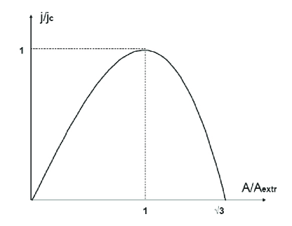
Figure 1: Schematic representation of the current density $j$ in the channel as function of the vector potential $A$.

Let us study the stability of the found homogeneous current state of NSC with respect to growing current. As is well known, it is determined by the behavior of the eigenvalues of the operator obtained by linearization of “equations of motion”, in our case, Eqs. (2). The state becomes absolutely unstable when the lowest eigenvalue turns to zero (see, for example, Ref. O01 ). In order to find corresponding value of the vector potential let us present the functions $\left\{\Delta,A\right\}$ in the form $\left\{\Delta_{0}+\Delta_{1},A+A_{1}\right\}$ assuming $\Delta_{1}\ll\Delta_{0},A_{1}\ll A$ and  linearize the system (2).

For the fixed current value the corrections $\left\{\Delta_{1},A_{1}\right\}$ are connected by the simple relation $A_{1}=-2A\left(\Delta_{1}/\Delta_{0}\right).$ This relation follows directly from the first equation of the system (3). Substituting it to the first equation of  the system (2) one can write the required equation for the eigenvalue $\lambda:$

$$\left[-\tau-\frac{3\pi\mathcal{D}e^{2}}{2Tc^{2}}\mathbf{A}^{2}+\frac{21\zeta\left(3\right)}{8\pi^{2}T^{2}}\Delta_{0}^{2}\left(A\right)\right]\Delta_{1}=\lambda\Delta_{1}.$$

Remaining in the left-hand side value $\Delta_{0}^{2}$ can be expressed in terms of  the vector potential in accordance to Eq. (3), which results in

$$\lambda\left(A\right)=2\tau-\frac{3\pi\mathcal{D}e^{2}}{Tc^{2}}A^{2}=2\tau\left[1-\left(\frac{A}{A_{\mathrm{extr}}}\right)^{2}\right].$$ (4)

The eigenvalue $\lambda$ becomes zero when the vector potential reaches its critical value $A=A_{\mathrm{extr}}.$ This is exactly the point of the absolute instability, where the activation energy in Arrenius law should turn zero.

Activation energy in decay rate of the NSC. The system (2) at a given current value has the second, inhomogeneous, solution $\Delta\left(A,x\right)$( $x$ is the coordinate along the channel), which determines the value of activation energy in Arrenius law. In order to find it let us exclude the vector potential from Eqs. (2). One finds

$$\left(\frac{\partial\Delta}{\partial x}\right)^{2}+\frac{4j^{2}T^{2}}{\pi^{2}\nu^{2}e^{2}\mathcal{D}^{2}\Delta^{2}}+\frac{8T\tau}{\pi\mathcal{D}}\Delta^{2}-\frac{7\zeta\left(3\right)\Delta^{4}}{2\pi^{3}\mathcal{D}T}=C$$ (5)

where $C=const$. Using the dimensionless variables

$$j=j_{\mathrm{c}}\Gamma,\;\Delta^{2}\left(\Gamma,x\right)=\Delta_{0}^{2}{}\left(\Gamma\right)Z\left(x\right),\;\Delta_{0}^{2}{}\left(\Gamma\right)=\Delta_{00}^{2}\mathcal{L}\left(\Gamma\right)\emph{,}$$ (6)

one finds from Eqs. (2) the cubic equation for $\mathcal{L}$

$$\mathcal{L}^{3}-\mathcal{L}^{2}+\frac{4}{27}\Gamma^{2}=0.$$ (7)

In the range $A<A_{\mathrm{extr}}$ Eq. (7) has the only physically meaningful solution

$$\mathcal{L}=\frac{1}{3}+\frac{2}{3}\sin\left[\frac{\pi}{6}+\frac{2}{3}\arcsin\sqrt{1-\Gamma^{2}}\right].$$ (8)

The value

$$C=\frac{8T\tau\Delta_{0}^{2}{}\left(\Gamma\right)}{\pi\mathcal{D}}\left\{\frac{4\Gamma^{2}}{27\mathcal{L}^{2}}+1-\frac{\mathcal{L}}{2}\right\}$$

can be found from Eq. (5) by applying the boundary conditions at infinity: $\Delta\left(\infty\right)=0$ and $\partial\Delta/\partial x|_{x\rightarrow\infty}=0.$

Let us note that the solution of Eq. (5) should be even with respect to any fixed point $x_{0}:$ $\Delta\left(x-x_{0}\right)=\Delta\left(x_{0}-x\right).$ It is why we can assume $x_{0}=0$ and solve Eq. (5) for $x>0$ with a boundary condition$\quad\partial\Delta/\partial x|_{x=0}=0.$ Such solution reads as

$$4\sqrt{\frac{T\tau\mathcal{L}}{\pi\mathcal{D}}}x=\int_{2\left(\mathcal{L}^{-1}-1\right)}^{Z}\frac{dz_{1}}{\left(1-z_{1}\right)\sqrt{z_{1}-2\left(\mathcal{L}^{-1}-1\right)}}.$$

Final integration results in

$$Z\left(x\right)=\frac{1-\mathcal{L}}{\mathcal{L}}+\frac{3\mathcal{L}-2}{\mathcal{L}}\tanh^{2}\left(2x\sqrt{\frac{T\tau\left(3\mathcal{L}-2\right)}{\pi\mathcal{D}}}\right).$$ (9)

One can see that corresponding $\Delta\left(\Gamma,x\right)$ is reduced to the one of the Ref. LA67 only when the flowing current is zero ($\Gamma=0,\mathcal{L}=1$).

Substituting $\Delta^{2}\left(\Gamma,x\right)$ found above to Eq. (1) and using Eqs. (6)-(8) we obtain the expression for activation energy $\delta F$

$$\delta F =4\nu S\int_{0}^{\infty}dx\left[\tau\Delta_{0}^{2}{}\left(1-Z\right)-\frac{7\zeta\left(3\right)\Delta_{0}^{4}}{16\pi^{2}T^{2}}\left(1-Z^{2}\right)\right]$$

$$-4\nu S\tau\Delta_{0}^{2}{}\left(1-\mathcal{L}\right)\int_{0}^{\infty}dx\left(\frac{1}{Z}-1\right).$$ (10)

Simple integration leads to the final expression for activation energy, valid for an arbitrary bias current:

$$\delta F =2\nu\tau\Delta_{00}^{2}{}\left(\tau\right)S\sqrt{\frac{\pi\mathcal{D}}{T\tau}}\mathcal{L}\left[\frac{\sqrt{\left(3\mathcal{L}-2\right)}}{3\mathcal{L}}\right.$$

$$\left.-\frac{\sqrt{1-\mathcal{L}}}{\sqrt{2}}\arctan\left(\sqrt{\frac{3\mathcal{L}-2}{2\left(1-\mathcal{L}\right)}}\right)\right].$$ (11)

When the bias current is close to its critical value one can find from Eqs.(9)-(10) that $3\mathcal{L}-2=\frac{2}{\sqrt{3}}\sqrt{1-\Gamma^{2}}$ and the expression for activation energy is noticeably simplified:

$$\delta F=\delta F_{0}\cdot\mathcal{L}\left(\Gamma\right)\left[\frac{9}{20}\left(\frac{2}{\sqrt{3}}\sqrt{1-\Gamma^{2}}\right)^{5/2}\right],$$ (12)

where

$$\delta F_{0}=\left(2/3\right)\nu\tau\Delta_{00}^{2}{}\left(\tau\right)S{}\sqrt{\frac{\pi\mathcal{D}}{T\tau}}$$ (13)

is the value of activation energy at zero current ($\Gamma=0$).

Let us emphasize that in Ref. LA67 the activation energy in Arrenius law tends to non-zero constant when current reaches its critical value. The latter constant differs only by the numerical coefficient of the order of one from the value of activation energy Eq. (13) calculated at zero current. At the same time, one can clearly see from Eq. (12) the dramatic effect on $\delta F$ of the correct account for flowing current. Indeed, the current dependent factor in square brackets strongly depletes the activation energy Eq. (12) with respect to $\delta F_{0}$. Even not too close to the critical current when $\sqrt{1-\Gamma^{2}}\approx 1/3$ the activation energy given by Eq. (12) is 30 times smaller then prediction of the Ref. LA67 . (see Fig. 2).

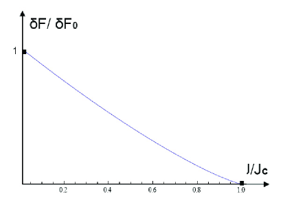
Figure 2: Current dependence of the activation energy. $\delta F\left(J\right)$

Let us indicate the interesting property of the current dependent factor in the general Eq. (11) exposed by square brackets. In the vicinity of the critical current two first terms of its Taylor expansion are exactly canceled out (see Eq. (12)). Cancelation of the first term in Eq. (11) can be foreseen and seems trivial, while the second cancelation, which results in the additional decrease of activation energy $\delta F$ with respect to $\delta F_{0}$, is surprising.

Pre-exponential factor. Let us move to estimation of the pre-exponential factor in Arrenius law for the number of voltage jumps per unit time. The GL formalism does not allow its exact definition: in order to do this it is necessary to know at least the dynamical equations for the order parameter valid in the wide range of frequencies. Other possibility is to know the shape of $J-V$ characteristic of the NSC above the critical current, for $J-J_{\mathrm{c}}\ll J_{\mathrm{c}}.$ Nevertheless, the simplest way to evaluate the pre-exponential factor is the dimensional analysis which we will use below.

The Josephson relation Ref. J62 connects the average voltage $V$ at the channel to the average time interval $\Delta t$ between the voltage jumps: $eV=\pi\hbar/\left(\Delta t\right).$ The latter can be estimated as

$$\Delta t=\left(\frac{\pi\hbar}{k_{\mathrm{B}}\Delta_{00}\mathcal{L}^{1/2}}\right)\frac{1}{L}\sqrt{\frac{\pi\hbar\mathcal{D}}{k_{\mathrm{B}}T\tau\left(3\mathcal{L}-2\right)}}\exp\left(\frac{\delta F}{k_{\mathrm{B}}T}\right).$$ (14)

Indeed, the first factor should define the characteristic time scale. We choose it to be in the form $2\pi\hbar/k_{B}\Delta_{0}\left(\Gamma\right).$Then, one should take into account the existence of the “zero-mode”, i.e. the arbitrariness of the choice of $x_{0}.$ This means that the instability can arise in an arbitrary point of channel and it involves the domain of the size of coherence length. This results in appearance of the second factor in Eq. (14), which is nothing else as the ratio of the coherence length in the presence of current to the length $L$ of the channel. Finally, accounting for the Arrenius exponent we arrive at the Eq. (14).

At this point one can write down the J-V characteristics of the NSC close to transition temperature and for arbitrary current $J<J_{\mathrm{c}}:$

$$V\left(J\right)=\frac{k_{\mathrm{B}}\Delta_{00}\left(\tau\right)L}{e}\left(\frac{k_{\mathrm{B}}T\tau\left(3\mathcal{L}-2\right)\mathcal{L}}{\pi\hbar\mathcal{D}}\right)^{\frac{1}{2}}\exp\left(-\frac{\delta F}{k_{\mathrm{B}}T}\right).$$

Discussion.We demonstrated that the account for the effect of current flow through the NSC results in a strong suppression of the energy barrier for the phase slip events with respect to its value at zero current. In the general Eq. (11) not only the first term, proportional to $\left(1-J/J_{\mathrm{c}}\right)^{1/4}$, but also the next one, proportional to $\left(1-J/J_{\mathrm{c}}\right)^{3/4}$  are canceled close to the critical current $J_{\mathrm{c}}.$ As the result,  the first non-vanishing term turns out to be proportional $\left(1-J/J_{\mathrm{c}}\right)^{5/4}$, which is the reason of a strong reduction of  the barrier. Moreover, the additional numerical smallness arises due to the high order of Taylor expansion in Eq. (11). As a consequence the barrier reduction turns significant even for currents, being relatively far from the critical value: for $J_{\mathrm{c}}-J=0.1J_{\mathrm{c}}$ the reduction factor is 12.4.

One can estimate the width of the temperature smearing $\Delta T$ of the transition at fixed current $J$ just equating $\delta F\sim T_{c}.$ In the most interesting case $J\rightarrow J_{c}$ Eq. (12) gives

$$\Delta T\left(J\right)\sim\frac{\Delta T\left(J=0\right)}{\left(1-J/J_{\mathrm{c}}\right)^{5/6}},$$

where $\Delta T\left(J=0\right)\sim Gi_{\left(1\right)}$ (Ginzburg-Levanyuk number LV04 for the NSC) is the width of transition at zero current. This formula differs from the result of  Ref. LA67 parametrically, by $\left(1-J/J_{\mathrm{c}}\right)^{-5/6}$, which provides the necessary factor of the order of tens lacking in Ref. LA67 for the agreement with the experiment PG67 .

Let us mention that the discussed dissipation process is affine to the well studied phenomenon of the Josephson current decay due to the thermal phase fluctuations BP82 . The activation energy for the latter also turns zero when current, flowing through junction approaches the critical one:

$$\delta\emph{F}_{J}\sim\left(1-J/J_{\mathrm{c}}\right)^{3/2}.$$

The difference between exponents of $\ \delta\emph{F}_{J}$ and $\delta F$ (Eq. (12) is related to the additional dependence of the order parameter in NSC on current. This analogy can be useful when one is trying to understand what kind of the J-V characteristics one could expect for NSC when currents exceed the critical value ($J>J_{\mathrm{c}}$). Three different scenarios are possible after overcoming the potential barrier in Josephson junction (see Fig. 3) : (I) the system jumps to the neighbor minimum and for a long time remains around the new minimum (its phase changes by 2$\pi$); (II) the system switches to the regime of the “free over-barrier semiclassical motion”; (III) the system jumps to any other minimum with the phase change by 2$\pi N$ ($N$ is an integer number with some distribution function M ) and for a long time remains there.

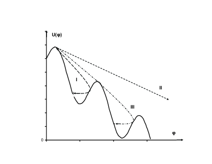
Figure 3: Different scenarios for the decay of a metastable state in Josephson junction.

The realization of this or that scenario depends on the values of the effective viscosity and $J/J_{\mathrm{c}}$ (depth of the potential well). One could expect possibility of realization of all this variety of options (depending on $J/J_{\mathrm{c}},T/T_{\mathrm{c}}$ and $l_{\mathrm{tr}}$) also in the supercritical regime of the J-V characteristics of the NSC. In experimental realization the first importance acquires the problem of overheating related to the very high current densities in superconductor.

The authors acknowledge financial support of the SIMTEC project in the frameworks of the YII Programme of European Community.

Yu.N.O. is grateful for hospitality of  “Tor Vergata” University of Rome (Italy) and grant of the RFBR.

References

- (1) J.S.Langer and Vinay Ambegaokar, Phys. Rev. 164, 498 (1967).
- (2) Michael Tinkham, Introduction to Superconductivity, McGraw-Hill Book Company, (1975).
- (3) A.A.Abrikosov, Fundamentals of the Theory of Metals, North Holland, (1988).
- (4) A.I.Larkin, A.A.Varlamov, Theory of fluctuations in superconductors, Oxford University Press, (2005).
- (5) R.D.Parks and R.P.Groff, Phys. Rev. Lett. 18, 342 (1967).
- (6) L.P.Gor’kov, Soviet Physics - JETP, 9, 1364 (1959).
- (7) Yu.N.Ovchinnikov Soviet Physics - JETP, 92, 858 (2001).
- (8) B.D.Josephson, Advances in Physics, 14, 419 (1965).
- (9) A.Barone, G.Paterno, Josephson effect: Physics and applications, John Wiley and Sons, NY, (1982).
- (10) V.I.Melnikov, Soviet Physics - JETP, 60, 380 (1984).