Thermal Effects on the Stability of Excited Atoms in Cavities

Abstract

An atom, coupled linearly to an environment, is considered in a harmonic approximation in thermal equilibrium inside a cavity. The environment is modeled by an infinite set of harmonic oscillators. We employ the notion of dressed states to investigate the time evolution of the atom initially in the first excited level. In a very large cavity (free space) for a long elapsed time, the atom decays and the value of its occupation number is the physically expected one at a given temperature. For a small cavity the excited atom never completely decays and the stability rate depends on temperature.

I Introduction

Inhibition of spontaneous emission by confined atoms is a well-known phenomenon, currently related to the dipole orientation with respect to parallel mirrors or to the relation between the size of the confining device and the emission wavelength (see for instance farina1 ; farina2 and other references therein). The theoretical understanding of these and other effects in atomic physics on perturbative grounds requires the calculation of very high-order terms in perturbative series, that makes the standard Feynman diagram technique practically unreliable. This has lead to trials of treating non-perturbativelly such kind of systems using the semi-quantitative idea of a dressed atom bouquinCohen . However serious difficulties, due to nonlinearity, are present to get rigorous results in these approaches. A way to circumvent these mathematical difficulties is to assume that under certain conditions the coupled atom-electromagnetic field system may be approximated by a system composed of a harmonic oscillator coupled linearly to the field modes through some effective coupling constant $g$. This is the case for linear response theory in $QED$, where the electric dipole interaction gives the leading contribution to the radiation process Wylie ; Jhe . Although a linear model is a simple theory, it permits a better understanding of the need for non-perturbative analytical treatment of coupled systems. This is the basic problem underlying the idea of dressed quantum mechanical operators.

The perturbative treatment of interacting systems is carried out by considering bare, non-interacting fields. The interaction is taken into account order by order in powers of the coupling constant. However there are situations where the use of perturbation theory is not reliable, as in the low energy domain of quantum chromodynamics and resonant effects in atomic physics, associated with the coupling of atoms with strong radiofrequency fields bouquinCohen .

The idea of a bare particle associated to a bare matter field is actually an artifact of perturbation theory. A charged physical particle is always coupled to the gauge field, i.e, it is always “dressed” by a cloud of quanta of the gauge field (photons, in the case of electrodynamics). In a simplified model for a radiating atom, a way to treat directly dressed objects, has been introduced. This is the method of dressed states and dressed coordinates adolfo1 that has been employed in several cases adolfo2 ; adolfo3 ; adolfo4 ; adolfo5 ; adolfo6 .

In this paper we generalize the zero-temperature formulation, dealing non-perturbatively with the inhibition of spontaneous emission adolfo2 ; adolfo3 , to finite temperature. The objective is to consider the stability of confined excited atoms in an environment at finite temperature.

II The model

We start by considering a bare atom approximated by a harmonic oscillator described by the bare coordinate and momentum $q_{0},p_{0}$ respectively, having bare frequency $\omega_{0}$, linearly coupled to a set of $N$ other harmonic oscillators (the environment) described by bare coordinate and momenta $q_{k},p_{k}$ respectively, with frequencies $\omega_{k}$, $k=1,2,\ldots,N$. The limit $N\rightarrow\infty$ will be taken later. A model of this type, describing a linear coupling of a particle with an environment, has been used for years in several situations, for instance to study the quantum Brownian motion of a particle with the path-integral formalism zurek ; paz ; caldeira ; caldeira1 . The whole system is supposed to reside inside a spherical cavity of radius $R$ in thermal equilibrium with the environment, at a temperature $T=\beta^{-1}$ ($k_{B}$, the Boltzmann constant is taken equal to 1).

The Hamiltonian for such a system is written in the form,

$$H=\frac{1}{2}\left[p_{0}^{2}+\omega_{0}^{2}q_{0}^{2}+\sum_{k=1}^{N}\left(p_{k}^{2}+\omega_{k}^{2}q_{k}^{2}\right)\right]-q_{0}\sum_{k=1}^{N}c_{k}q_{k},$$ (1)

where the $c_{k}$’s are coupling constants. In the limit $N\rightarrow\infty$, we recover the case of an atom coupled to the environment, after redefining divergent quantities, in a manner analogous to mass renormalization in field theories.

The Hamiltonian (1) is transformed to the principal axis by means of a point transformation,

$$q_{\mu}=\sum_{r=0}^{N}t_{\mu}^{r}Q_{r}\;\;,\,p_{\mu}=\sum_{r=0}^{N}t_{\mu}^{r}P_{r}\,,$$ (2)

where $\mu=(0,\{k\})\,\;\;k=1,2,...,N$, performed by an orthonormal matrix $T=(t_{\mu}^{r})$. The subscripts $\mu=0$ and $\mu=k$ refer respectively to the atom and the harmonic modes of the reservoir and $r$ refers to the normal modes. In terms of normal momenta and coordinates, the transformed Hamiltonian reads

$$H=\frac{1}{2}\sum_{r=0}^{N}(P_{r}^{2}+\Omega_{r}^{2}Q_{r}^{2}),$$

where the $\Omega_{r}$’s are the normal frequencies corresponding to the stable collective oscillation modes of the coupled system. It can be shown adolfo1 that

$$t_{k}^{r}=\frac{c_{k}}{\omega_{k}^{2}-\Omega_{r}^{2}}t_{0}^{r}\;,\;\;t_{0}^{r}=\left[1+\sum_{k=1}^{N}\frac{c_{k}^{2}}{(\omega_{k}^{2}-\Omega_{r}^{2})^{2}}\right]^{-\frac{1}{2}},$$ (3)

with the condition

$$\omega_{0}^{2}-\Omega_{r}^{2}=\sum_{k=1}^{N}\frac{c_{k}^{2}}{\omega_{k}^{2}-\Omega_{r}^{2}}.$$ (4)

To correctly describe the coupling of the atom with the field, we take

$$c_{k}=\eta\omega_{k}\,;\;\;\;\;\;\eta=\sqrt{2g\Delta\omega},$$ (5)

where $g$ is a constant with dimension of frequency. It measures the strength of the coupling; $\Delta\omega=\pi c/R$ is the interval between two neighboring frequencies of the reservoir and frequencies of the field modes are given by adolfo1 ,

$$\omega_{k}=k\Delta\omega=k\frac{\pi c}{R}$$ (6)

The sum in Eq. (4) diverges for $N\rightarrow\infty$. This makes the equation meaningless, unless a renormalization procedure, analogous to mass renormalization in field theories, is implemented Thirring . Adding and subtracting a term $\eta^{2}\Omega_{r}^{2}$ in the numerators of the right hand side in Eq. (4) we have

$$\bar{\omega}^{2}-\Omega_{r}^{2}=\eta^{2}\Omega_{r}^{2}\sum_{k=1}^{\infty}\frac{1}{\omega_{k}^{2}-\Omega_{r}^{2}},$$ (7)

where we define the renormalized frequency

$$\bar{\omega}^{2}=\omega_{0}^{2}-\delta\omega^{2}=\lim_{N\rightarrow\infty}(\omega_{0}^{2}-N\eta^{2}).$$ (8)

We find that the addition of a counterterm $-\delta\omega^{2}q_{0}^{2}$ in the Hamiltonian Eq. (1) compensates the divergence of $\omega_{0}^{2}$ in such a way as to leave a finite, physically meaningful renormalized frequency $\bar{\omega}$.

Using the formula,

$$\sum_{k=1}^{\infty}\frac{1}{(k^{2}-u^{2})}=\left[\frac{1}{2u^{2}}-\frac{\pi}{u}{\rm cot}(\pi u)\right],$$ (9)

Eq. (7) can be rewritten as (dropping the label for the eigenfrequencies),

$$\cot\left(\frac{R\Omega}{c}\right)=\frac{\Omega}{2\pi g}+\frac{c}{2R\Omega}\left(1-\frac{R\bar{\omega}^{2}}{\pi gc}\right).$$ (10)

This gives an infinity of solutions. The spectrum of the collective normal modes is denoted by $\Omega_{r}\,;\;\;r=0,1,2,\cdots$. The transformation matrix elements are adolfo1 ,

$$t_{0}^{r} = \frac{\eta\Omega_{r}}{\sqrt{(\Omega_{r}^{2}-\bar{\omega}^{2})^{2}+\frac{\eta^{2}}{2}(3\Omega_{r}^{2}-\bar{\omega}^{2})+\pi^{2}g^{2}\Omega_{r}^{2}}},$$

$$t_{k}^{r} = \frac{\eta\omega_{k}}{\omega_{k}^{2}-\Omega_{r}^{2}}t_{0}^{r}.$$ (11)

Unless explicitly stated, the limit $N\rightarrow\infty$ is understood in the following.

III Dressed states

Let us consider the eigenstates of our system, $\left|n_{0},n_{1},n_{2}...\right\rangle$, represented by the normalized eigenfunctions in terms of the normal coordinates $\{Q_{r}\}$,

$$\phi_{n_{0}n_{1}n_{2}...}(Q)=\prod_{s}\left[\sqrt{\frac{2^{n_{s}}}{n_{s}!}}H_{n_{s}}\left(\sqrt{\frac{\Omega_{s}}{\hbar}}Q_{s}\right)\right]~{}\Gamma_{0},$$ (12)

where $H_{n_{s}}$ stands for the $n_{s}$-th Hermite polynomial and $\Gamma_{0}$ is the normalized ground state eigenfunction,

$$\Gamma_{0}(Q)={\cal{N}}\exp\left[-\frac{1}{2\hbar}\sum_{r=0}^{\infty}\Omega_{r}Q_{r}^{2}\right].$$ (13)

We introduce dressed coordinates $q_{0}^{\prime}$ and $\{q_{k}^{\prime}\}$ for, respectively, the dressed atom and the dressed field, defined by,

$$\sqrt{\bar{\omega}_{\mu}}q_{\mu}^{\prime}=\sum_{r}t_{\mu}^{r}\sqrt{\Omega_{r}}Q_{r},$$ (14)

where $\bar{\omega}_{\mu}=\{\bar{\omega},\;\omega_{k}\}$. In terms of dressed coordinates, we define for the time $\tau=0$, the dressed states, $\left|\kappa_{0},\kappa_{1},\kappa_{2}...\right\rangle$ by means of the complete orthonormal functions

$$\psi_{\kappa_{0}\kappa_{1}...}(q^{\prime})=\prod_{\mu}\left[\sqrt{\frac{2^{\kappa_{\mu}}}{\kappa_{\mu}!}}H_{\kappa_{\mu}}\left(\sqrt{\frac{\bar{\omega}_{\mu}}{\hbar}}q_{\mu}^{\prime}\right)\right]\Gamma_{0},$$ (15)

where $q_{\mu}^{\prime}=\left\{q_{0}^{\prime},\,q_{k}^{\prime}\right\}$, $\bar{\omega}_{\mu}=\{\bar{\omega},\,\omega_{k}\}$. Notice that the ground state, $\Gamma_{0}$, in the above equation is the same as in Eq. (12). The invariance of the ground state is due to our definition of dressed coordinates given by Eq. (14). In fact, we get the normal coordinates $Q_{r}$ in terms of the dressed ones from Eq. (14). Replacing them in Eq. (13) we find that the ground state in terms of the dressed coordinates has the form

$$\Gamma_{0}(q^{\prime})={\cal{N}}\exp\left[-\frac{1}{2\hbar}\sum_{\mu=0}^{\infty}\bar{\omega}_{\mu}q_{\mu}^{\prime 2}\right].$$ (16)

Each function $\psi_{\kappa_{0}\kappa_{1}...}(q^{\prime})$ describes a state in which the dressed oscillator $q_{\mu}^{\prime}$ is in its $\kappa_{\mu}$-th excited state.

It is worthwhile to note that our dressed coordinates are new objects, different from both the bare coordinates, $q$, and the normal coordinates $Q$. In particular, the dressed states, although being collective objects, should not be confused with the eigenstates given by Eq. (12). While the eigenstates $\phi$ are stable, all the dressed states $\psi$ are unstable, except for the ground state $\Gamma_{0}$. The important idea is that the dressed states are physically meaningful.

In this framework, we write the physical states in terms of dressed annihilation and creation operators $a_{\mu}^{\prime}$ and $a_{\mu}^{\prime{\dagger}}$ defined in terms of dressed coordinates and momenta in the usual way,

$$a_{\mu}^{\prime} = \sqrt{\frac{\bar{\omega}_{\mu}}{2}}q_{\mu}^{\prime}+\frac{i}{\sqrt{2\bar{\omega}_{\mu}}}p_{\mu}^{\prime}$$ (17)

$$a_{\mu}^{\prime{\dagger}} = \sqrt{\frac{\bar{\omega}_{\mu}}{2}}q_{\mu}^{\prime}-\frac{i}{\sqrt{2\bar{\omega}_{\mu}}}p_{\mu}^{\prime}\;.$$ (18)

Then the initial dressed density operator corresponding to the thermal bath is given by

$$\rho^{\prime}_{\beta}=\frac{1}{Z^{\prime}_{\beta}}\exp\left[-\hbar\beta\sum_{k=1}^{\infty}\omega_{k}\left(a_{k}^{\prime{\dagger}}a_{k}^{\prime}+\frac{1}{2}\right)\right],$$ (19)

with $Z^{\prime}_{\beta}=\prod_{k}z_{\beta}^{k\prime}$ being the partition function of the dressed reservoir, where

$$z_{\beta}^{k\prime}={\rm Tr}\left[e^{-\hbar\beta\omega_{k}\left(a_{k}^{\prime{\dagger}}a_{k}^{\prime}+1/2\right)}\right].$$ (20)

The system evolves with time ($\tau$). The time-dependent dressed occupation numbers are defined as

$$n_{\mu}^{\prime}(\tau)={\rm Tr}\left(a_{\mu}^{\prime{\dagger}}(\tau)a_{\mu}^{\prime}(\tau)\rho_{0}^{\prime}\otimes\rho_{\beta}^{\prime}\right)$$

(the prime is to clearly distinguish the dressed quantities from the bare ones), where $\rho_{0}^{\prime}$ is the density operator for the dressed atom; $a_{\mu}^{\prime}(\tau)$ and $a_{\mu}^{\prime{\dagger}}(\tau)$ are the time-dependent creation and annihilation operators.

The time evolution of the dressed annihilation operator is given by,

$$\frac{d}{d\tau}a_{\mu}^{\prime}(\tau)=i\left[{H},a_{\mu}^{\prime}(\tau)\right]\;$$ (21)

and a similar equation for $a_{\mu}^{\prime{\dagger}}(\tau)$. We solve this equation with the initial condition at time $\tau=0$,

$$a_{\mu}^{\prime}(0)=\sqrt{\frac{\omega_{\mu}}{2}}q_{\mu}^{\prime}+\frac{i}{\sqrt{2\omega_{\mu}}}p_{\mu}^{\prime}.$$ (22)

which, in terms of bare coordinates, becomes

$$a_{\mu}^{\prime}(0)=\sum_{r,\nu=0}^{N}\left(\sqrt{\frac{\Omega_{r}}{2}}t_{\mu}^{r}t_{\nu}^{r}q_{\nu}+\frac{it_{\mu}^{r}t_{\nu}^{r}}{\sqrt{2\Omega_{r}}}p_{\nu}\right)\;.$$ (23)

We assume a solution for $a_{\mu}^{\prime}(\tau)$ of the type

$$a_{\mu}^{\prime}(t)=\sum_{\nu=0}^{\infty}\left(\dot{B}_{\mu\nu}^{\prime}(\tau){q}_{\nu}+B_{\mu\nu}^{\prime}(\tau){p}_{\nu}\right)\;.$$ (24)

Using Eq. (1) we find,

$$B_{\mu\nu}^{\prime}(\tau)=\sum_{r=0}^{\infty}t_{\nu}^{r}\left(a_{\mu}^{\prime r}e^{i\Omega_{r}\tau}+b_{\mu}^{\prime r}e^{-i\Omega_{r}\tau}\right)\;.$$ (25)

The initial conditions for $B_{\mu\nu}^{\prime}(\tau)$ and $\dot{B}_{\mu\nu}^{\prime}(\tau)$ are obtained by setting $t=0$ in Eq. (24) and comparing with Eq. (23); then

$$B_{\mu\nu}^{\prime}(0) = i\sum_{r=0}^{\infty}\frac{t_{\mu}^{r}t_{\nu}^{r}}{\sqrt{2\Omega_{r}}}\;,$$ (26)

$$\dot{B}_{\mu\nu}^{\prime}(0) = \sum_{r=0}^{\infty}\sqrt{\frac{\Omega_{r}}{2}}t_{\mu}^{r}t_{\nu}^{r}\;.$$ (27)

Using these initial conditions and the orthonormality of the matrix $\{t_{\mu}^{r}\}$ we obtain $a_{\mu}^{\prime r}=0$, $b_{\mu}^{\prime r}=it_{\mu}^{r}/\sqrt{2\Omega_{r}}$. Replacing these values for $a_{\mu}^{\prime r}$ and $b_{\mu}^{\prime r}$ in Eq. (25) we get

$$B_{\mu\nu}^{\prime}(\tau)=i\sum_{r=0}^{\infty}\frac{t_{\mu}^{r}t_{\nu}^{r}}{\sqrt{2\Omega_{r}}}e^{-i\Omega_{r}t}\;.$$ (28)

We have

$$a_{\mu}^{\prime}(\tau) = \sum_{r,\nu=0}^{\infty}t_{\mu}^{r}t_{\nu}^{r}\left(\sqrt{\frac{\Omega_{r}}{2}}{q}_{\nu}+\frac{i}{\sqrt{2\Omega_{r}}}{p}_{\nu}\right)e^{-i\Omega_{r}\tau}$$ (29)

$$= \sum_{r,\nu=0}^{N}t_{\mu}^{r}t_{\nu}^{r}\left(\sqrt{\frac{\omega_{\nu}}{2}}{q}_{\nu}^{\prime}+\frac{i}{\sqrt{2\omega_{\nu}}}{p}_{\nu}^{\prime}\right)e^{-i\Omega_{r}\tau}$$

$$= \sum_{\nu=0}^{\infty}f_{\mu\nu}(\tau){a}_{\nu}^{\prime}\;,$$

where

$$f_{\mu\nu}(\tau)=\sum_{r=0}^{\infty}t_{\mu}^{r}t_{\nu}^{r}e^{-i\Omega_{r}\tau}\,$$ (30)

with $\mu\,,\nu=0,\,\{k\}$, $k=1,2,\cdots$.

This leads to the time evolution equation for the dressed occupation number of the atom termalizacao ; livro ,

$$n_{0}^{\prime}(\tau)=|f_{00}(\tau)|^{2}n_{0}^{\prime}+\sum_{k=1}^{\infty}|f_{0k}(\tau)|^{2}n_{k}^{\prime}\,,$$ (31)

where $n_{0}^{\prime}$ stands for the occupation number at $\tau=0$.

IV Thermal effects in a small cavity

In this section we consider the weak coupling regime, defined by

$$g=\bar{\omega}\alpha,,$$ (32)

where $\alpha$ is the fine-structure constant.

With $\eta=\sqrt{2g\pi c/R}$ and defining the dimensionless parameter

$$\delta=\frac{g}{\Delta\omega}=\frac{gR}{\pi c},$$ (33)

Eq. (10) becomes,

$$\cot\left(\frac{\pi\Omega\delta}{g}\right)=\frac{\Omega}{2\pi g}+\frac{g}{2\pi\delta\Omega}\left(1-\frac{\delta\bar{\omega}^{2}}{g^{2}}\right).$$ (34)

Let us consider the right hand side of Eq. (34) such that

$$\frac{\delta\bar{\omega}^{2}}{g^{2}}>1.$$ (35)

In the weak coupling regime, this corresponds to a value of $\delta$, $\delta\gtrsim 5.3\times 10^{-5}$. For a frequency $\bar{\omega}=4.0\times 10^{14}/s$ (in the visible red) this gives a condition on the cavity size of $R\gtrsim 1.7\times 10^{-8}\,m$. Then the general behavior of the solutions of Eq. (34) is illustrated in Fig(1). We find that all but one of the eigenfrequencies are very close to the frequencies of the field modes, $\omega_{k}$, given by Eq. (6). Then we label solutions for the eigenfrequencies $\Omega_{r}$ as, $\Omega_{0}$, $\Omega_{k}$, $k=1,2,\cdots$. The solutions $\Omega_{k}$ of Eq. (34) are,

$$\Omega_{k}=\frac{\pi c}{R}\left(k+\epsilon_{k}\right)\,\;\;k=1,2,\ldots\,,$$ (36)

with $0<\epsilon_{k}<1$, satisfying the equation,

$$\mathrm{cot}(\pi\epsilon_{k})=\frac{2c}{gR}(k+\epsilon_{k})+\frac{1}{(k+\epsilon_{k})}\left(1-\frac{\bar{\omega}^{2}R}{\pi gc}\right).$$ (37)

Since every $\epsilon_{k}$ is much smaller than $1$, Eq. (37) can be linearized in $\epsilon_{k}$, giving,

$$\epsilon_{k}=\frac{\pi gcRk}{\pi^{2}c^{2}k^{2}-\bar{\omega}^{2}R^{2}}.$$ (38)

The eigenfrequencies, $\Omega_{k}$, are obtained by solving Eqs. (36) and (37) or (38).

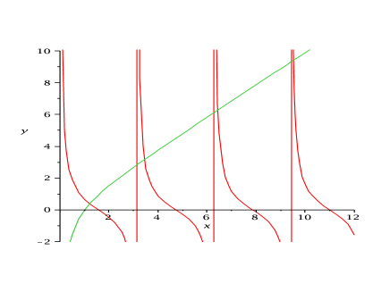
Figure 1: Solutions of Eq. (34), for cavities satisfying the condition Eq. (35); the asymptotes of the cotangent curve correspond to the frequencies of the field modes $\omega_{k}$.

The lowest eigenfrequency, $\Omega_{0}$, is obtained by assuming that it satisfies the condition $\Omega_{0}R/c\ll 1$. Inserting this condition in Eq. (34) and keeping up to quadratic terms in $\Omega$ we obtain the solution for the lowest eigenfrequency,

$$\Omega_{0}\approx\bar{\omega}\left(1-\frac{\pi\delta}{2}\right).$$ (39)

Consistency between Eq. (34) and the condition $\Omega_{0}R/c\ll 1$ gives a condition on $R$, $i.e$ $R\ll(c/g)\lambda$, with $\lambda=(\pi/2)\left(g/\bar{\omega}\right)^{2}$.

Let us first determine the temperature independent term $|f_{00}(\tau)|^{2}n_{0}^{\prime}$ in Eq. (31), considering that the dressed atom is initially (at $\tau=0$) in the first excited level, that is $n_{0}^{\prime}=1$. We evaluate $(t_{0}^{0})^{2}$ and $(t_{0}^{k})^{2}$ from Eqs. (11), (36), (38), and (39) to find

$$(t_{0}^{k})^{2}\approx\frac{2gR}{\pi ck^{2}}=\frac{2\delta}{k^{2}},$$ (40)

and then using the normalization condition $\sum_{r=0}^{\infty}(t_{0}^{r})^{2}=1$ and $\zeta(2)=\sum_{k=1}^{\infty}k^{-2}=\pi^{2}/6$, we have

$$(t_{0}^{0})^{2}\approx 1-\frac{\pi gR}{3c}=1-\frac{\pi^{2}\delta}{3}$$ (41)

From Eq. (30), using the de Moivre formula, $e^{i\theta}=\cos\theta+i\sin\theta$, we have

$$|f_{\mu\nu}(\tau)|^{2}=\sum_{r,s=0}^{\infty}t_{\mu}^{r}t_{\nu}^{r}t_{\mu}^{s}t_{\nu}^{s}\cos(\Omega_{r}-\Omega_{s})\tau.$$ (42)

Let us assume that the thermal bath is at zero temperature, $i.e.$ all the modes of the reservoir are in the ground state, $n_{k}^{\prime}=0$ for all values of $k$. Taking the above approximations for $t_{0}^{k}$ and $t_{0}^{0}$, we get from Eq. (31), the zero-temperature time evolution of the occupation number of the dressed atom initially in the first excited level,

$$|f_{00}(\tau)|^{2}\approx\left(1-\frac{\pi^{2}\delta}{3}\right)^{2}+4\delta\left(1-\frac{\pi^{2}\delta}{3}\right)\sum_{k=1}^{\infty}\frac{1}{k^{2}}\cos(\Omega_{k}-\Omega_{0})\tau+4\delta^{2}\sum_{k,l=1}^{\infty}\frac{1}{k^{2}l^{2}}\cos(\Omega_{k}-\Omega_{l})\tau.$$ (43)

This is an oscillating function which has a minimum value $\mathrm{Min}(|f^{00}(t)|^{2})$. Taking both cosine functions in Eq. (43) equal to $-1$, we get a lower bound for $\mathrm{Min}(|f^{00}(t)|^{2})$ given, up to first order in $\delta$, by

$$F(\delta)=1-\left(\frac{2\pi^{2}}{3}-2\right)\delta.$$ (44)

As an example we consider that the atom in the first excited state has an emission frequency $\bar{\omega}\approx 4\times 10^{14}/s$, in the visible red, and we take the radius of the confining cavity $R\approx 10^{-6}$m. With these data we get $F(\delta)\approx 0.99$, that is a probability of $99\%$ at zero temperature, that it will almost never decay. This shows the high stability of the system, which is confirmed by experiment Haroche3 ; Hulet .

In order to take into account the temperature effects, we must consider the second term in Eq. (31), that is we must evaluate the quantity

$$|f_{0k}(\tau)|^{2}=|t_{0}^{0}t_{k}^{0}e^{-i\Omega_{0}\tau}+\sum_{l=1}^{\infty}t_{0}^{l}t_{k}^{l}e^{-i\Omega_{l}\tau}|^{2}.$$ (45)

This is carried out by using the matrix elements obtained from Eq. (11) and the formulas for eigenfrequencies in a small cavity.

It is assumed that the thermal distribution of the occupation numbers of the field modes in the cavity follow the Bose-Einstein distribution,

$$n_{k}^{\prime}=\frac{1}{e^{\hbar\beta\omega_{k}}-1}.$$ (46)

This can be justified in the following way: in the case of an arbitrarily large cavity, the dressed field modes coincide with the bare ones adolfo1 , which in the limit of vanishing coupling makes this approximation exact. Strictly speaking this is not the case for a finite cavity. Nevertheless, in many situations this approximation is acceptable in the weak coupling régime. For instance a cavity of radius $R\approx 10^{-6}m$ is $\sim 10^{4}$ times larger than the size of a hydrogen atom (the Bohr radius). In such a case the atom “sees” the cavity to be a very large one and the approximation is justified. Then from Eqs. (45)and (31), we get the time evolution of the temperature dependent occupation number for the atom,

$$n_{0}^{\prime}(\tau,\beta)=|f_{00}(\tau)|^{2}n_{0}^{\prime}+\sum_{k=1}^{\infty}\frac{1}{e^{(\hbar\beta\pi c/R)k}-1}\left[(t_{0}^{0})^{2}(t_{k}^{0})^{2}+2\sum_{l=1}^{\infty}t_{0}^{0}t_{0}^{l}t_{k}^{0}t_{k}^{l}\cos(\Omega_{0}-\Omega_{l})\tau+\sum_{l,n=1}^{\infty}t_{0}^{l}t_{0}^{n}t_{k}^{l}t_{k}^{n}\cos(\Omega_{l}-\Omega_{n})\tau\right]\\$$

where $|f_{00}(\tau)|^{2}$ is given by Eq. (43). The matrix elements $t_{k}^{0}$ and $t_{k}^{l}$ in the above formulas are evaluated from Eqs. (11), (36) and (39) to be,

$$t_{k}^{0}=\frac{k\,g^{2}\sqrt{2\delta}}{k^{2}g^{2}-\Omega_{0}^{2}\delta^{2}}\,;\;\;t_{k}^{l}=\frac{2k\delta}{k^{2}-(l+\epsilon_{l})^{2}}\frac{1}{l}.\\$$

The occupation number $n_{0}^{\prime}(\tau,\beta)$ is an oscillating function which has a minimum value, ${\rm{Min}}[n_{0}^{\prime}(\tau,\beta)]$, that depends on the temperature $\beta^{-1}$. We can obtain a lower bound, $n_{0}^{\prime}(\beta)$, for this minimum, such that ${\rm{Min}}[n_{0}^{\prime}(\tau,\beta)]>n_{0}^{\prime}(\beta)$, by taking both cosine functions in Eq. (IV) equal to $-1$

$$n_{0}^{\prime}(\beta)=F(\delta)n_{0}^{\prime}+\sum_{k=1}^{\infty}\frac{1}{e^{(\hbar\beta\pi c/R)k}-1}\left[(t_{0}^{0})^{2}(t_{k}^{0})^{2}-2\sum_{l=1}^{\infty}t_{0}^{0}t_{0}^{l}t_{k}^{0}t_{k}^{l}-\sum_{l,n=1}^{\infty}t_{0}^{l}t_{0}^{n}t_{k}^{l}t_{k}^{n}\right].$$ (47)

Numerical calculation of Eqs. (IV) and (47) will describe how the time evolution of the occupation number and the stability of the excited atom are affected by heating. We take for the plots $n_{0}^{\prime}=1$, that is the atom initially in the first excited level.

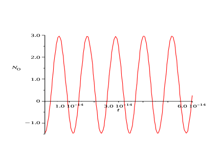
Figure 2: Time evolution of the thermal dependent occupation number $n_{0}^{\prime}(\tau,\beta)$ for a temperature $T=300\,K\,$; the scale for the vertical axis is $N_{0}=(n_{0}-1)\times 10^{-12}$; time is in seconds.

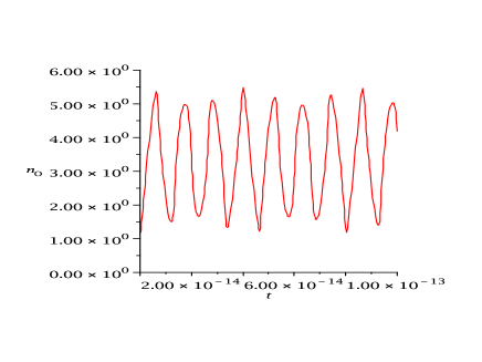
Figure 3: Time evolution of the thermal dependent occupation number $n_{0}^{\prime}(\tau,\beta)$ for a temperature $T=10^{5}\,K$; time is in seconds.

Figure 4: Temperature behavior of the lower bound for the minimum of $n_{0}^{\prime}(\tau,\beta)$, $n_{0}^{\prime}(\beta)$, given by Eq. (47); temperature is in Kelvin.

In Fig. (2) and in Fig. (3) the time evolution of the temperature dependent occupation number $n_{0}^{\prime}(\tau,\beta)$ is plotted for some representative values of the emission frequency and the temperature. In Fig. (4) the lower bound for its minimum, $n_{0}^{\prime}(\beta)$, is plotted as a function of temperature. We find from these figures that raising temperature increases the amplitude of oscillation of the occupation number and that its minimum lower bound, $n_{0}^{\prime}(\beta)$, also grows with temperature. For a given emission frequency $\bar{\omega}=4.0\times 10^{14}/s$, the increase of the amplitude of oscillation of $n_{0}^{\prime}(\tau,\beta)$ and of its lower bound $n_{0}^{\prime}(\beta)$ are negligible for room temperatures, they are significant for high laboratory temperatures. In Fig. (3) $n_{0}^{\prime}(\tau,\beta)$ is plotted for $T=10^{5}\,K$ ($\sim 8.4\,eV$); although this temperature is very high for everyday life, it can, in principle, be attained in laboratory for excited atoms. In fact it is lower than the ionization temperature of $13.6\,eV$ for the hydrogen atom, and still much lower than the nuclear fusion temperature of $\approx 10^{8}\,K$ ($\sim 8.4\,KeV$). We find that the average occupation number at this temperature ($T=10^{5}\,K$) is about $3.5$ times higher than the zero temperature value $n_{0}^{\prime}(\tau,T=0)\approx 1$. At room temperature the occupation number will remain very close to the zero-temperature value, as is shown in Fig. (2). Therefore we find that as the temperature is raised, both the amplitude of oscillation of the occupation number and its minimum, grow with respect to the zero-temperature values.

V Concluding remarks

At zero temperature the dressed atom, initially in the first or higher excited state, can only decay, since all field modes are in the ground state. It is inhibited from decaying by confinement in a cavity of small size. However at finite temperature, the field modes in the cavity can be in excited states with a finite probability given by the Bose-Einstein distribution function. As a consequence the dressed atom can exchange quanta from the field. This means that the thermal occupation number of excited states of the atom increases with temperature. In other words, as an effect of heating the atom will be in a higher excited state which may be able to decay. However the decay is inhibited by the confining geometry. The results presented above give sufficient proof of these ideas.

This behavior is also to be contrasted with the situation of an arbitrarily large cavity (free space) described in termalizacao ; livro . In that case, for long times the dressed occupation number of the atom approaches smoothly to an asymptotic value which is nearly the one obtained from the Bose distribution at the equilibrium temperature of the reservoir. Taking the same value as before for $\bar{\omega}$, this value is $n_{0}^{\prime}(t\rightarrow\infty,\beta;\bar{\omega},R\rightarrow\infty)=1/(e^{14}-1)\approx 0$. In that case the growth of the Bose-Einstein weight factor due to raising temperature is compensated by the lowering due to larger and larger values of $R$, leading to an equilibrium occupation number.

References

• (1) C. Farina, T. N. C. Mendes, F. S. S. Rosa and A. Tenorio, Phys. Rev. A 78, 012105 (2008).
• (2) C. Farina and T. N. C. Mendes, J. Phys A: Math. Gen. 40, 7343 (2007).
• (3) C. Cohen-Tannoudji, ”Atoms in Electromagnetic Fields”, (World Scientific, Singapure, 1994).
• (4) J. M. Wylie and J. E. Sipe, Phys. Rev. A 30, 1185 (1984).
• (5) W. Jhe and K. Jang, Phys. Rev. A 53, 1126 (1996).
• (6) N. P. Andion, A. P. C. Malbouisson and A. Mattos Neto, J. Phys. A: Math. Gen. 34, 3735, (2001).
• (7) G. Flores-Hidalgo, A. P. C. Malbouisson and Y. W. Milla, Phys. Rev. A 65, 063414 (2002).
• (8) G. Flores-Hidalgo and A. P. C. Malbouisson, Phys. Rev. A 66, 042118 (2002).
• (9) A. P. C. Malbouisson, Annals of Physics 308, 373 (2003).
• (10) G. Flores-Hidalgo and A. P. C. Malbouisson, Phys. Lett. A 337, 37 (2005).
• (11) G. Flores-Hidalgo, C.A. Linhares, A.P.C. Malbouisson and J.M.C. Malbouisson, J. Phys. A: Math. Ther. 41, 075404 (2008).
• (12) W. G. Unruh and W. H. Zurek, Phys. Rev. D 40, 1071 (1989).
• (13) B. L. Hu, J. P. Paz and Y. Zhang, Phys. Rev. D 45, 2843 (1992).
• (14) A. O. Caldeira and A. J. Leggett, Ann. Phys. (N.Y) 149, 374 (1983).
• (15) M. Rosenau da Costa, A. O. Caldeira, S. M. Dutra and H. Westfahl Jr., Phys. Rev A 61, 022107 (2000).
• (16) W. Thirring and F. Schwabl, Ergeb. Exakt. Naturw. 36, 219 (1964).
• (17) W. Jhe, A. Anderson, E. A. Hinds, D. Meschede, L. Moi and S. Haroche, Phys. Rev. Lett. 58, 666 (1987).
• (18) R.G. Hulet, E. S. Hilfer and D. Kleppner, Phys. Rev. Lett. 55, 2137 (1985).
• (19) G. Flores-Hidalgo, A. P. C. Malbouisson, J. M. C. Malbouisson, Y. W. Milla and A. E. Santana, Phys. Rev. A (Online), 79, 032105 (2009).
• (20) F. C. Khanna, A. P. C. Malbouisson, J. M. C. Malbouisson and A. E. Santana, Thermal Quantum Field Theory - Algebraic Aspects and Applications, 1. ed. (World Scientific, Singapore, 2009).