Phonons and the coherence scale of models of heavy fermions

Abstract

We consider models of heavy fermions in the strong coupling or local moment limit and include phonon degrees of freedom on the conduction electrons. Due to the large mass or low coherence temperature of the heavy fermion state, it is shown that such a regime is dominated by vertex corrections which leads to the complete failure of the Migdal theorem. Even at weak electron-phonon couplings, binding of the conduction electrons competes with the Kondo effect and substantially reduces the coherence temperature, ultimately leading to the Kondo breakdown. Those results are obtained using a combination of the slave boson method and Migdal-Eliashberg approximation as well as the dynamical mean-field theory approximation.

I Introduction and Models

The heavy fermion paramagnetic state as realized for instance in CeCu₆ or induced by a weak magnetic field in YbRh₂(Si_1-xGe_x)₂ corresponds to the coherent, Bloch like, superposition of the individual Kondo screening clouds of the spins of rare-earths.lohneysen08 The coherence temperature $T_{\rm coh}$, or inverse effective mass of this state is set by the Kondo Ueda86 ; Georges00 ; Pruschke00 ; Assaad04a scale which lies orders of magnitude below the Fermi temperature, $T_{F}$, of the host metallic state. In general, for weakly correlated metals, the characteristic phonon frequencies set by the Debye temperature $\Theta_{D}$ are much smaller than the Fermi temperature $E_{F}\simeq 10^{4-5}$K thus yielding a small parameter $\Theta_{D}/T_{F}$ on which Migdal theorem is based. Migdal58 This small parameter is absent in heavy fermion materials since the Fermi temperature should be replaced by $T_{\rm coh}$ which might be even smaller than 1K. Moreover, smallness of the relevant energy scales implies that properties of the ground state can be easily tuned by Hamiltonian perturbations. This observation raises the central question of this paper: what role do phonons play in models of heavy fermions?

We address this question on the basis of the periodic Anderson model (PAM) on a square lattice with Holstein phonons that couple to the conduction band electrons:

$$H= H_{0}+H_{V}+H_{ph}\text{ with }$$ (1)

$$H_{0}= \sum_{\boldsymbol{k},\sigma}\epsilon({\boldsymbol{k}})c^{\dagger}_{{\boldsymbol{k}},\sigma}c_{{\boldsymbol{k}},\sigma},$$

$$H_{V}= V\sum_{\boldsymbol{i},\sigma}\bigl{(}f^{\dagger}_{{\boldsymbol{i}},\sigma}c_{{\boldsymbol{i}},\sigma}+h.c.\bigr{)}+(\epsilon_{f}-\mu)\sum_{{\boldsymbol{i}},\sigma}f^{\dagger}_{{\boldsymbol{i}},\sigma}f_{{\boldsymbol{i}},\sigma}$$

$$+ U\sum_{\boldsymbol{i}}\bigl{(}n^{f}_{{\boldsymbol{i}},\uparrow}-1/2\bigr{)}\bigl{(}n^{f}_{{\boldsymbol{i}},\downarrow}-1/2\bigr{)},$$

$$H_{ph}= g\sum_{{\boldsymbol{i}}}\hat{Q}_{\boldsymbol{i}}(n^{c}_{{\boldsymbol{i}}}-1)+\sum_{\boldsymbol{i}}\Bigl{(}\frac{\hat{P}_{\boldsymbol{i}}^{2}}{2M}+\frac{k}{2}\hat{Q}_{\boldsymbol{i}}^{2}\Bigr{)}.$$

Here, $H_{0}$ describes the conduction band with dispersion relation $\epsilon({\boldsymbol{k}})=-2t(\cos k_{x}+\cos k_{y})-\mu$ and with $c^{\dagger}_{{\boldsymbol{k}},\sigma}$ creating a conduction electron with $z$-component of spin $\sigma$ and in the Bloch state with crystal momentum ${\boldsymbol{k}}$. Next, $H_{V}$ accounts for the hybridization with a conduction electron in Wannier state centered around unit cell ${\boldsymbol{i}}$ and the localized $f$-electron in the same unit cell while the Coulomb repulsion set by the Hubbard $U$ on the $f$-orbitals accounts for local moment formation. Finally, $H_{ph}$ corresponds to Einstein phonons with a Holstein coupling to the conduction electrons. In fact, the choice between a model in which phonons couple predominately either to the conduction or $f$-electrons is material dependent. Indeed, retaining the coupling of Holstein phonons only to the conduction electrons is justified in the local moment regime where charge fluctuations on the $f$-orbitals are suppressed due to the strong Coulomb repulsion. In this limit the model maps onto the Kondo lattice model (KLM):

$$H_{KLM}=H_{0}+H_{ph}+J\sum_{\boldsymbol{i}}{\boldsymbol{S}}_{\boldsymbol{i}}^{c}{\boldsymbol{S}}_{\boldsymbol{i}}^{f}.$$ (2)

In contrast, the effect of phonon coupling to the $f$-electrons is expected to become more important in the mixed valence regime of moderately heavy fermions such as filled skutterudites as emphasized in Ref. Ono05, .

We use several methods to unravel the physics contained in those model Hamiltonians. Arbitrarily low temperatures as well as phonon frequencies may be reached within a combination of the slave-boson (SB) mean-field approximation Kotliar86 with the self-consistent calculation of the self-energy diagram of Fig. 1 within Migdal-Eliashberg Migdal58 ; Eliashberg60 ; Engelsberg63 (ME) approximation. The former leads to the hybridized band picture of the heavy fermion state while the latter allows one to account for coupling to the phonons. Furthermore, since the SB approximation fails at finite temperatures while the ME approach does not capture vertex corrections, we equally use the dynamical mean-field theory (DMFT) approximation with a recently developed weak coupling continuous-time quantum Monte Carlo (CT-QMC) impurity solverRubtsov05 to include phonon degrees of freedom into the PAM. Assaad07 ; Assaad08 Finally, in order to access the low temperature limit, we resort to numerical renormalization group (NRG) method Bulla08 as a complementary to the CT-QMC impurity solver applied to the KLM (2).

To understand the failure of the ME approximation for the heavy fermion state, let us start with the phonons coupled to a band of conduction electrons with a flat density of states of width $W$. In this case, the self-energy diagram of Fig. 1 gives a mass renormalization,

$$\frac{m^{*}}{m_{0}}=1+\lambda\left(1-\frac{\omega_{0}}{W/2+\omega_{0}}\right)\text{ where }\lambda=\frac{g^{2}}{kW}$$ (3)

and $\omega_{0}=\sqrt{k/M}$ corresponds to the phonon frequency, and $m_{0}$ is the mass of the bare electron. $\lambda$ corresponds to the dimensionless electron-phonon interaction and we have explicitly included high frequency corrections.

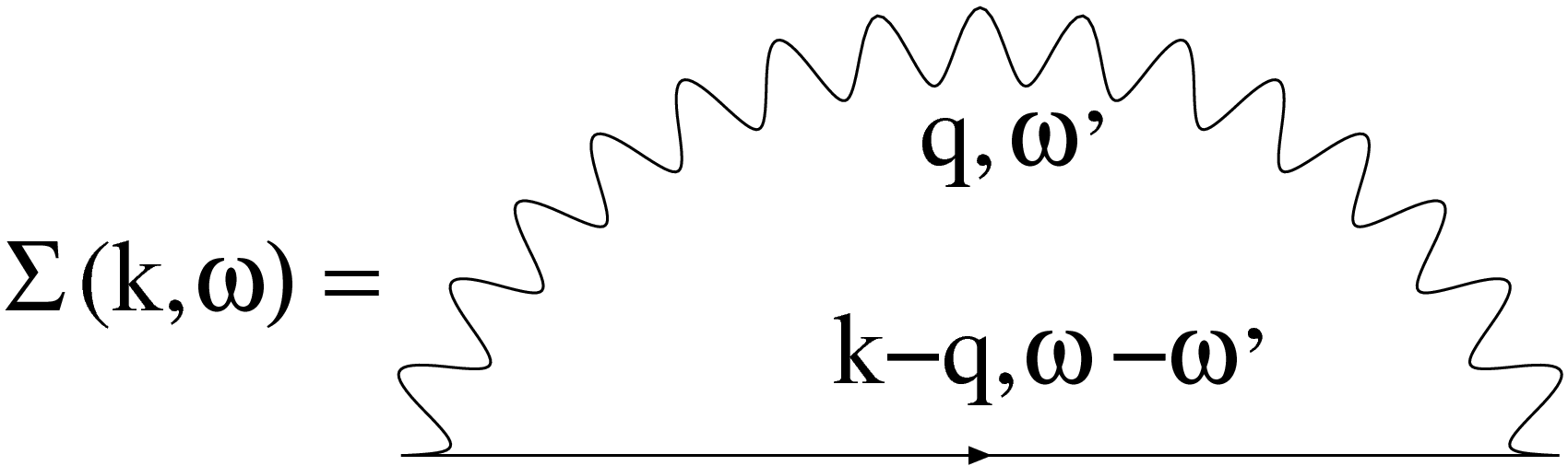
Figure 1: Self-energy diagram. The solid (wavy) line corresponds to the bare single-particle Green’s function (phonon propagator), respectively.

In the adiabatic limit $\omega_{0}<<T_{\rm coh}$, we can use the above formula with the heavy Fermi liquid as a starting point rather than the bare conduction electrons to account for the effect of phonons. As it is reviewed in some details in Sec. II, the ratio of the coherence temperature of the heavy fermion state to the Fermi temperature of the host metal is given by the quasiparticle (QP) residue,

$$Z=|\langle\Psi^{N-1}_{0}|c_{{\boldsymbol{k}}_{F},\sigma}|\Psi^{N}_{0}\rangle|^{2}.$$ (4)

This quantity measures the overlap of the QP with a bare conduction electron. Hence, the coupling of the phonons to the heavy fermion quasiparticles will be renormalized by a factor $Z$ in comparison to the coupling to the bare electron (i.e. $g\rightarrow gZ$). One equally expects effective bandwidth to be scaled by the same factor Z. Accounting for these two renormalization factors, and neglecting the high frequency correction in Eq. (3) gives a mass enhancement,

$$\frac{m^{*}}{m}\simeq 1+\lambda Z,$$ (5)

where $m\simeq m_{0}/Z$ corresponds to the effective mass of the heavy fermion state in the absence of phonons. Therefore, in this limit the coherence scale,

$$T_{\rm coh}\propto\frac{m_{0}}{m^{*}}\simeq\frac{Z}{1+\lambda Z},$$ (6)

is next to unaffected by the inclusion of phonons since $Z<<1$ even in the strong electron-phonon coupling limit, $\lambda\simeq 1$. In Sec. II we verify explicitly this result with the use of a combination of the SB technique and the ME approximation. In this case the coherence temperature is also protected from adiabatic phonons which stems from their coupling to merely a fraction, $Z$, of the heavy QP.

In the high frequency limit, $W>>\omega_{0}>>T_{coh}$ the correct starting point is to consider the Hamiltonian $H_{0}+H_{ph}$. Neglecting vertex corrections, one can account for the low energy physics of this Hamiltonian within the ME approximation. This approximation describes the formation of quasiparticles with enhanced effective mass set by $m_{0}(1+\lambda)$ or equivalently a bandwidth reduced by a factor $(1+\lambda)$. From there onwards one can account for the magnetic impurities. The hybridization matrix element between the QP and the $f$-electron is renormalized by a factor $1/\sqrt{1+\lambda}$ in comparison to the hybridization with the bare electron. Taking into account those two renormalization factors, bandwidth and hybridization, the Kondo temperature, $T_{K}\propto\exp(-UW/4V^{2})$, remains invariant at this level of approximation. Hence, as in the adiabatic case, one also expects in this regime a very weak influence of the phonon degrees of freedom on the scales of the heavy fermion state. This point is confirmed explicitly in Sec. II within the ME approximation.

Therefore, we anticipate that retaining only non crossing diagrams thus omitting vertex corrections leaves the scales of the heavy fermion state next to unaffected. Vertex corrections will clearly play a role since they lead to polaron binding which competes with the Kondo screening of the impurity spins. In particular, integrating out the phonon degrees of freedom yields a retarded attractive interaction. The retardation is set by $1/\omega_{0}$ and its magnitude by $\lambda W/2$. This term leads to binding between polarons into singlets and is responsible for the onset of superconductivity. To capture this competition and associated substantial reduction of the coherence temperature even at very low values of the electron phonon coupling, we carry out in Sec. III DMFT calculations using two complementary impurity solvers based on: (i) a recently developed CT-QMC techniqueRubtsov05 ; Assaad07 as well as (ii) zero-temperature NRG method.Bulla08 Finally, in Sec. IV we conclude and discuss the implications of our results.

Unless stated otherwise, throughout the paper we consider the parameters $U/t=4$, $V/t=1$, and $\epsilon_{f}=\mu$ for the PAM and $J=W/2$ with $W=0.2$ for the KLM, and choose the chemical potential $\mu$ such that the total particle number per unit cell reads $\langle n\rangle=1.8$.

II Mean-field approximation

In order to understand the basic underlying physics of the model Eq. (1) it is instructive to work first in the mean-field framework. A good starting point to handle strong electron correlations is offered by the SB mean-field method. Kotliar86 Indeed, its usefulness has been proved in the studies devoted to searching for the ground-state of both the doped Hubbard model Raczkowski06 and its multi-band variant. Fresard97 Moreover, it has been applied to determine instabilities of the PAM, pam_mag and since it captures two characteristic energy scales, i.e., the coherence $T_{\rm coh}$ and the Kondo $T_{\rm K}$ ones, is believed to account for the essential physics of the heavy-fermion systems. Burdin09

Additionally, in order to gain preliminary insight into the interplay between electron correlations and electron-phonon coupling, we combine the SB technique with the ME approximation. Migdal58 ; Eliashberg60 ; Engelsberg63 Remarkably, despite obvious flaws there are some regimes where this approach works quite well Brunner00b ; Mishchenko01b ; Luscher06 and on top it might be systematically improved by including the leading-order vertex corrections in the self-energy calculations. For example, it has widely been used to describe the dynamics of a single hole in the magnetically ordered background of Mott insulators and to analyze changes in the QP properties by coupling to various bosonic excitations such as magnons, Martinez91 ; Ramsak98 phonons, Slezak06 ; Gunnarsson06 and orbitons. Brink00 Moreover, recent studies of the one-dimensional quarter-filled Holstein model have shown that in the temperature range above the onset of the Luttinger liquid phase, the approximation is capable of reproducing the temperature dependence of the one-particle spectral function obtained within a cluster extension of the DMFT. Assaad08

II.1 Energy scales in the PAM

It is now well established that both the PAM and its strong coupling version, i.e., the KLM have two paramagnetic solutions. The first one sets in above the scale $T_{\rm K}$ and is characterized by the fully localized $f$-electrons. In contrast, below the Kondo temperature $T_{\rm K}$, the $c$- and $f$-electrons couple to form a heavy fermion state that on decreasing $T$ evolves eventually into a coherent Fermi liquid state and the onset is marked by the so-called coherence scale $T_{\rm coh}$. Its most prominent features are: (i) a flat low-intensity region in the $c$-electron spectral function $A_{c}({\bf k},\omega)$ that results from the hybridization between a dispersionless correlated $f$-band and a wide conduction $c$-band; as shown in Fig. 2 it crosses the Fermi level and hence it is responsible for a metallic character of the low-temperature ground-state; (ii) quasiparticles with a strongly renormalized effective mass $m/m_{0}\gg 1$, and (iii) linear specific heat $C_{v}=\gamma T$.

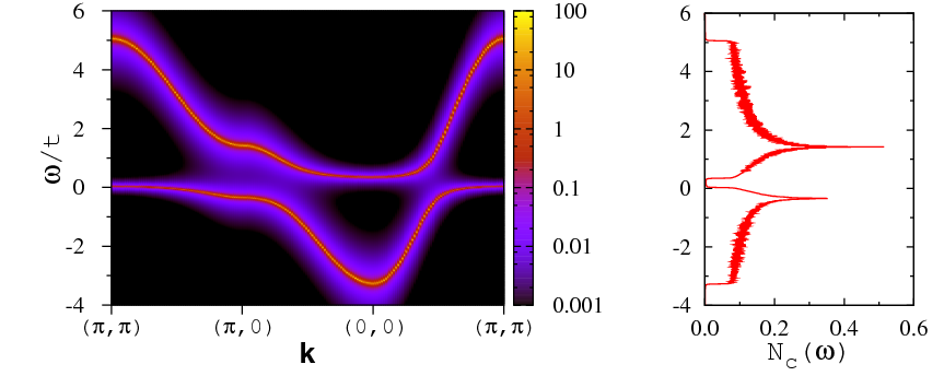
Figure 2: (Color online) $c$-electron spectral function $A_{c}({\bf k},\omega)$ (left) and the corresponding density of states $N_{c}(\omega)$ obtained in the PAM with $V/t=1$ in the coherent Fermi liquid regime at the low temperature $\beta t=400$.

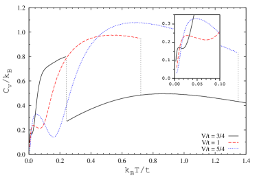
Figure 3: (Color online) Temperature dependence of the specific heat $C_{v}$: discontinuity of $C_{v}$ in the high-temperature regime signals Kondo breakdown at $T_{\rm K}$; low-temperature peaks indicate onset of the Fermi liquid regime at $T_{\rm coh}$. Inset shows a closeup of the low-temperature limit.

Within the SB approach one can define a Kondo temperature $T_{\rm K}$. It corresponds to the temperature scale at which the SB factor $z$ renormalizing the hybridization amplitude $V$ vanishes. The transition into the state with singly occupied $f$-orbitals at $T_{\rm K}$ is also seen as discontinuity of the specific heat $C_{v}=-T\bigl{(}\tfrac{\partial^{2}F_{SB}}{\partial T^{2}}\bigr{)}_{\langle n\rangle}$ shown in Fig. 3. The second feature of $C_{v}$ is a low-temperature peak at $T_{\rm coh}$ that signals entering the coherent Fermi liquid regime with well defined QP peaks whose effective mass is strongly enhanced. The two energy scales $T_{\rm coh}$ and $T_{\rm K}$ read off from Fig. 3 are listed in Table 1. As expected based on the Gutzwiller approach, Ueda86 large $N$-method, Georges00 DMFT studies, Pruschke00 as well as on the QMC simulations,Assaad04a one finds that both energy scales track each other on varying the hybridization amplitude $V$. To be more precise within the large $N$ approach, $T_{\rm coh}$ lies well below the Kondo temperature with proportionality constant being strongly dependent on the conduction density of states. However, at fixed density and upon varying the hybridization, $T_{\rm coh}$ tracks $T_{\rm K}$. In particular, for a flat density of states, the Gutzwiller method yields $T_{\rm K}\propto\exp(-UW/4V^{2})$ and accordingly increasing $V$ shifts both characteristic temperatures towards higher $T$. Remarkably, even though $T_{\rm K}$ changes by one order of magnitude on increasing $V/t$ from $3/4$ to $5/4$, the ratio $T_{\rm coh}/T_{\rm K}$ is next to constant (cf. Table 1).

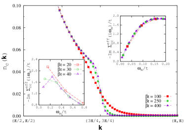
Figure 4: (Color online) $c$-electron single-particle occupation $n_{c}({\bf k})$ along the nodal direction of the Brillouin zone obtained in the PAM with $V/t=1$. Insets show the imaginary part of the effective $c$-electron self-energy $-{\rm Im}\Sigma_{cc}^{eff}(i\omega_{m})$ as a function of Matsubara frequencies $\omega_{m}$.

Table 1: Slave-boson coherence temperature $T_{\rm coh}$, Kondo temperature $T_{\rm K}$, their ratio, as well as QP residue $Z$ obtained from Eq. (7) in the PAM at $\beta t=400$ for a few representative values of the hybridization $V$.

$V/t$	$0.75$	$1.0$	$1.25$
$k_{B}T_{\rm coh}/t$	$0.010$	$0.026$	$0.046$
$k_{B}T_{\rm K}/t$	$0.244$	$0.721$	$1.346$
$T_{\rm coh}/T_{\rm K}$	$0.041$	$0.036$	$0.034$
$Z$	$0.018$	$0.043$	$0.066$

The onset of the coherent Fermi liquid is also signalized by the imaginary part of the effective $c$-electron self-energy $-{\rm Im}\Sigma_{cc}^{eff}(i\omega_{m})$ (see Appendix). Indeed, as shown in the inset in Fig. 4 with $V/t=1$, a conspicuous change in the behavior of $-{\rm Im}\Sigma_{cc}^{eff}(i\omega_{m})$ with $\omega_{m}\to 0$ takes place in the temperature region $30<\beta t<40$ matching the low-temperature peak in $C_{v}$. Moreover, a discontinuity in the $c$-electron single-particle occupation $n_{c}({\bf k})=\int_{-\infty}^{\mu}d\omega A_{c}({\bf k},\omega)$ emerges below $\beta t=100$ (see Fig. 4). In fact, since the coherent QP part of the spectral function is given at low temperature by a delta function of weight $Z$: $A_{c}({\bf k},\omega)\sim Z\delta(\omega-\varepsilon_{\bf k})$, its magnitude is given precisely by the QP residue $Z$ which in turn is directly related to the effective QP mass $Z^{-1}=m/m_{0}$. In the low temperature limit, the value of $Z$ can be determined as the slope of the imaginary part of the effective self-energy on the Matsubara axis (see the inset in Fig. 4):

$$Z=\left[1-\frac{{\rm Im}\Sigma_{cc}^{eff}(i\omega_{m})}{\omega_{m}}\right]^{-1}_{\omega_{m}=\pi T}.$$ (7)

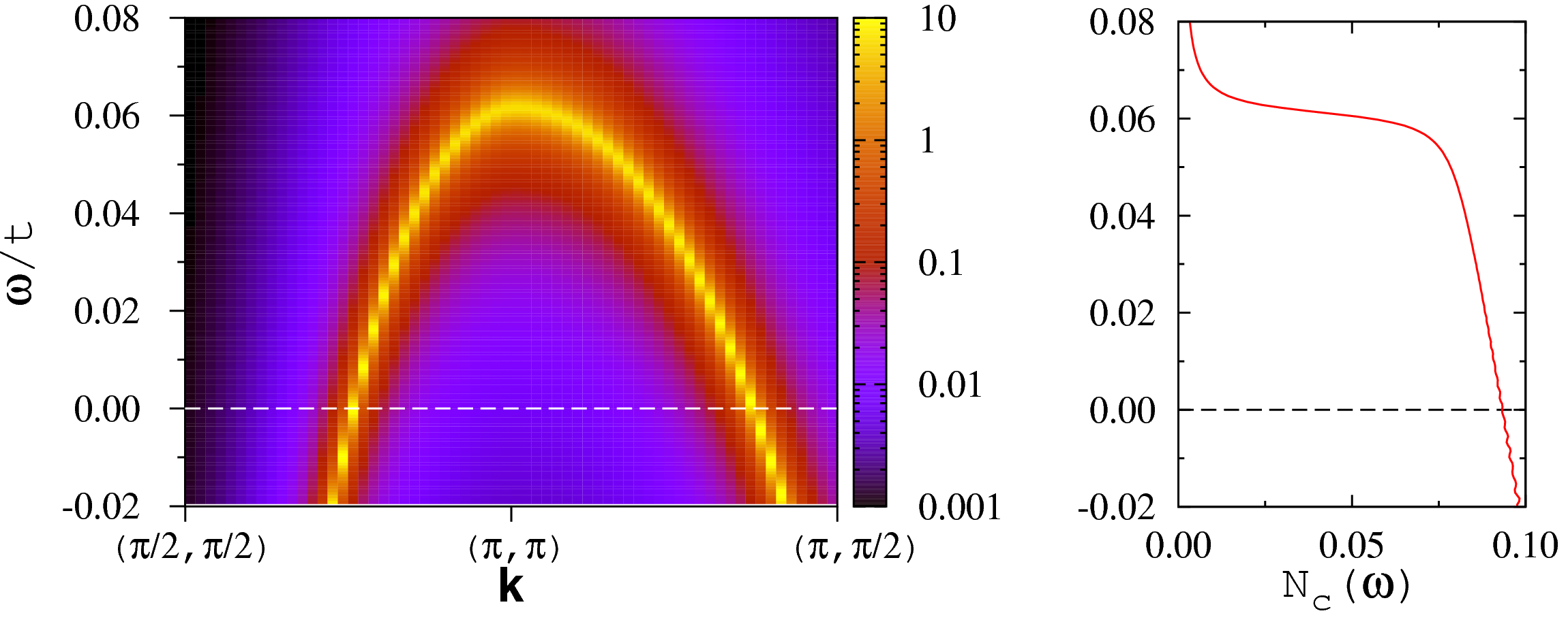
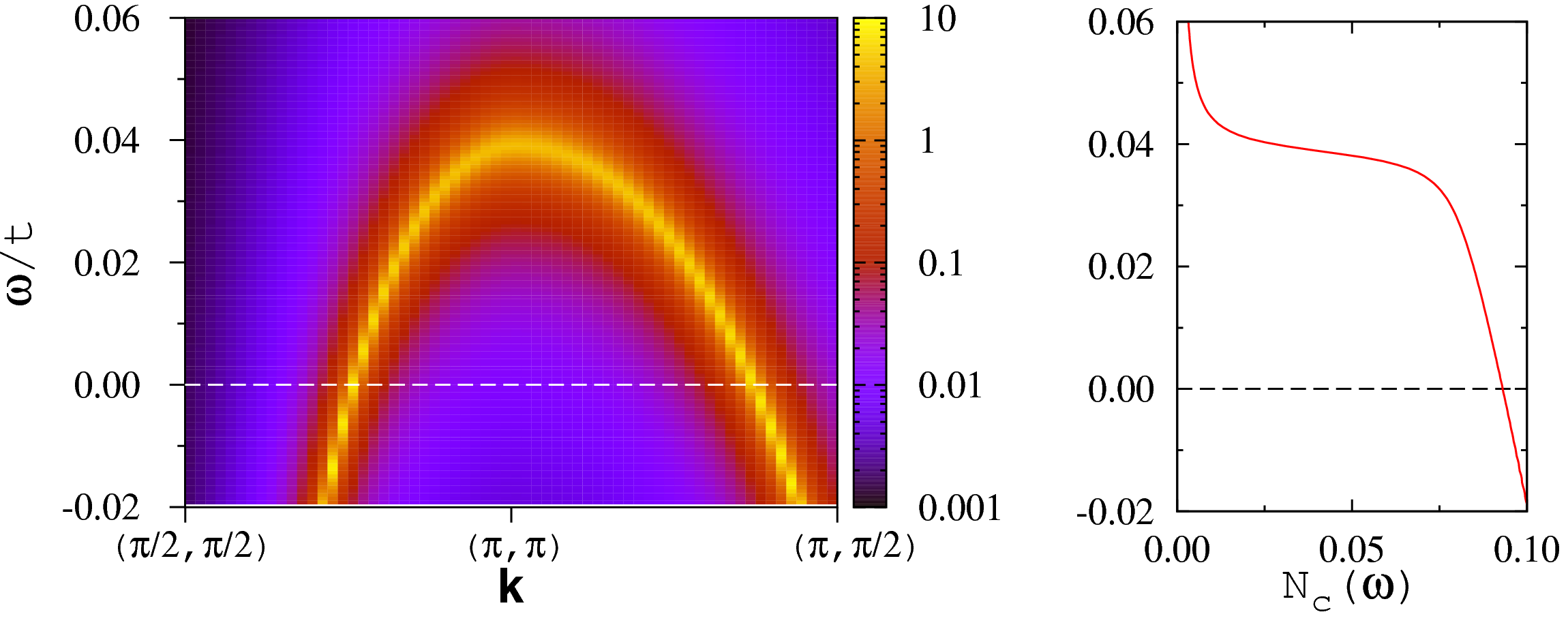
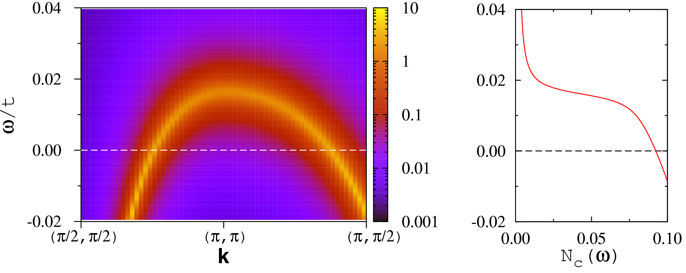
Figure 5: (Color online) Low-energy part of the $c$-electron spectral function $A_{c}({\bf k},\omega)$ (left) and the corresponding density of states $N_{c}(\omega)$ (right) in the PAM found at $\beta t=400$: $V/t=1.25$ (top), $V/t=1$ (middle), and $V/t=0.75$ (bottom).

Furthermore, we observe that the value of $V$ strongly influences the shape and the intensity of the QP band around the Fermi level depicted in Fig. 5. On the one hand, $V/t=5/4$ yields a more dispersive QP band with a higher intensity, as compared to the $V/t=1$ case. It extends much above the Fermi energy up to a certain value $\omega_{c}/t\simeq 0.06$. On the other hand, a smaller $V/t=3/4$ produces a strongly renormalized low-intensity flat band just above the Fermi level extending up to $\omega_{c}/t\simeq 0.02$. Hence, in the considered range of the hybridization amplitude $V$, the SB results indicate that both energy scales $T_{\rm coh}$ and $\omega_{c}$ are intimately related, i.e., $T_{\rm coh}\sim\omega_{c}$.

II.2 Effect of electron-phonon coupling

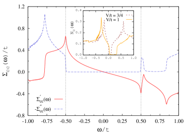
Figure 6: (Color online) Low-energy part of the real $\Sigma_{cc}^{\prime}(\omega)$ and imaginary $-\Sigma_{cc}^{\prime\prime}(\omega)$ part of the $c$-electron self-energy obtained with $V/t=1$, $\lambda=0.5$, and $\omega_{0}/t=0.5$ at $\beta t=400$. Inset depicts the corresponding $c$-electron density of states $N_{c}(\omega)$ and, for comparison, $N_{c}(\omega)$ obtained with $V/t=3/4$.

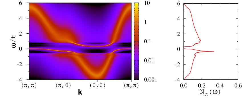
Figure 7: (Color online) Same as in Fig. 2 but with $\lambda=0.5$ and $\omega_{0}/t=0.5$.

We now discuss how the previously found features of the coherent ground state of the PAM are altered by the electron-phonon coupling. At zero temperature, the imaginary part of the self-energy of Eq. (31) reads,

$$\Sigma^{\prime\prime}_{cc}(\omega)=-\frac{g^{2}}{2k}\pi\omega_{0}\Bigl{\{}N_{c}^{+}\bigl{[}1-\Theta(\omega+\omega_{0})\bigr{]}+N_{c}^{-}\Theta(\omega-\omega_{0})\Bigr{\}},$$ (8)

with $N_{c}^{\pm}=N_{c}(\omega\pm\omega_{0})$ and $\Theta(\omega)$ being a usual Heavyside step function. Consequently, as shown in Fig. 6, $\Sigma^{\prime\prime}_{cc}(\omega)$ vanishes in a window $-\omega_{0}<\omega<\omega_{0}$. Moreover, the hybridization gap of the heavy fermion state, equally leads to strong suppression of this quantity just above $\omega>\omega_{0}$ (see Fig. 6). Away from this energy window the imaginary part of the self-energy is finite thereby producing an incoherent high-energy background visible in the single particle spectral function (see Fig. 7). A measure of this incoherent background is obtained from the value of $n_{c}({\boldsymbol{k}}=(\pi,\pi))$ shown in Fig.  8. Finally, since the imaginary part of the self energy vanishes at the Fermi energy, a well define QP is formed and the corresponding QP residue $Z$ can be extracted from the real part of self-energy,

$$\Sigma^{\prime}_{cc}(\omega)=-\frac{1}{\pi}{\mathcal{P}}\int_{-\infty}^{\infty}d\omega^{\prime}\frac{\Sigma^{\prime\prime}_{cc}(\omega^{\prime})}{\omega-\omega^{\prime}},$$ (9)

and with the use of Eq. (7).

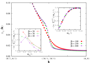
Figure 8: (Color online) Same as in Fig. 4 but with $\lambda=0.5$ and $\omega_{0}/t=0.5$.

We turn now to the most important aspect of our analysis namely the mass renormalization due to the inclusion of the rainbow diagrams. This quantity is plotted in Fig. 9 at $\lambda=0.5$ and as a function of phonon frequency $\omega_{0}$. Here one finds that in comparison to the free-electron case, shown as inset in Fig. 9(a), the overall mass renormalization is extremely small especially in the adiabatic case. As depicted in Fig. 10, this weak mass renormalization is also apparent in delicate flattening of the QP band producing very small shift in the peak position of the QP pole in the vicinity of ${\boldsymbol{k}}=(\pi,\pi)$.

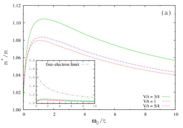
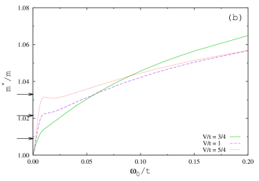
Figure 9: (Color online) Enhancement of the effective mass $m^{*}$ obtained for a fixed electron-phonon coupling $\lambda=0.5$ at $\beta t=400$ for representative values of the hybridization $V$. (a) Overall behavior of $m^{*}$. Inset: enhancement of $m^{*}$ in the heavy fermion state is marginal as compared to the free-electron limit. (b) Low-frequency limit $\omega_{0}/t\leq 0.2$. The arrows indicate $m^{*}$ estimated from Eq. (5).

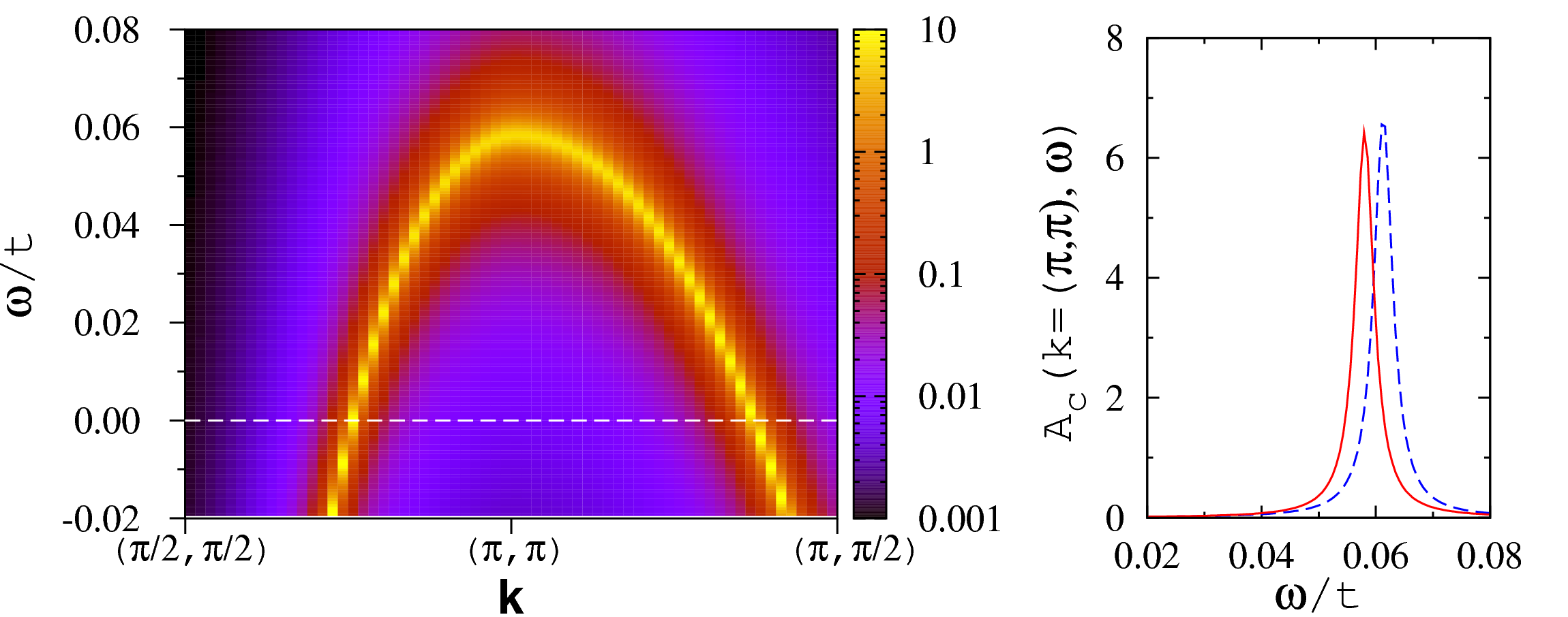
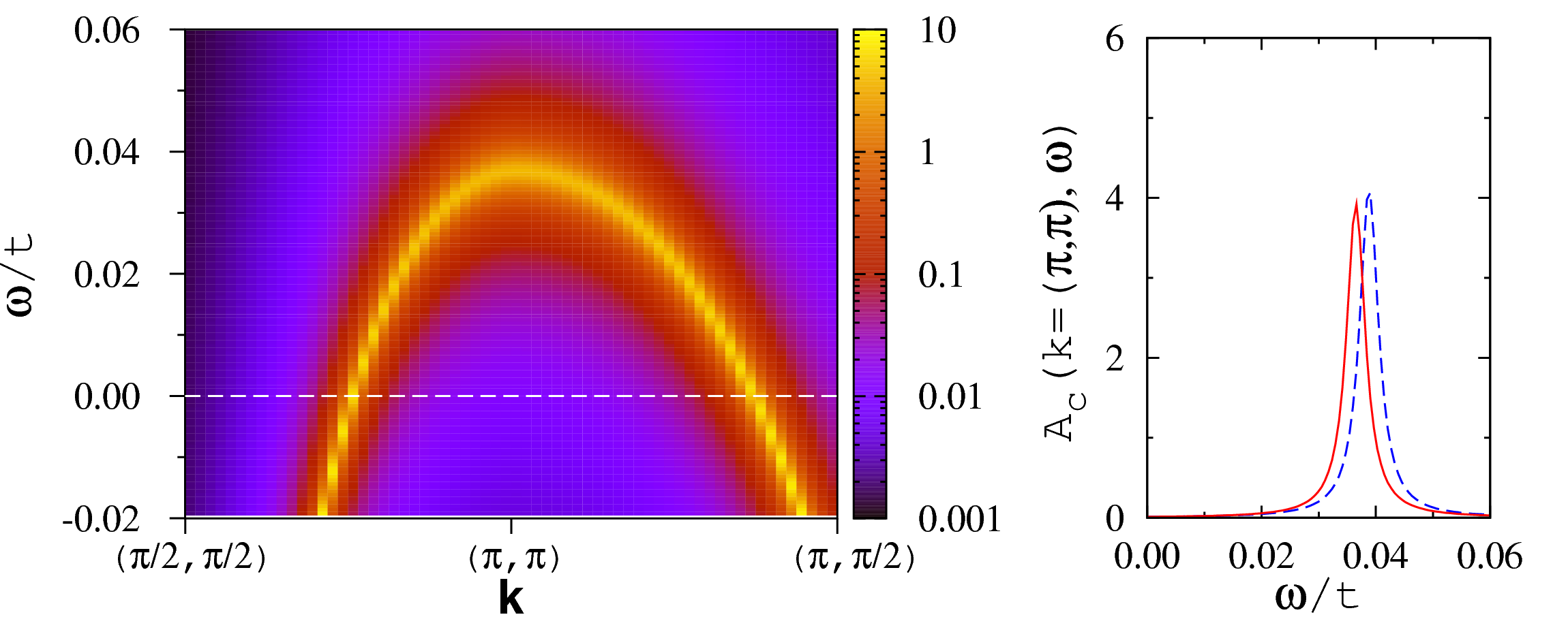
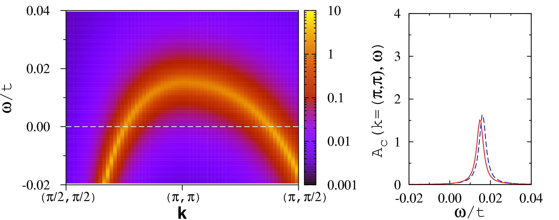
Figure 10: (Color online) Low-energy part of the $c$-electron spectral function $A_{c}({\bf k},\omega)$ (left) and the QP peak at ${\bf k}=(\pi,\pi)$ (right) obtained with $\lambda=0.5$ and $\omega_{0}/t=0.5$ at $\beta t=400$: $V/t=1.25$ (top), $V/t=1$ (middle), and $V/t=0.75$ (bottom). For comparison, the corresponding $A_{c}({\bf k}=(\pi,\pi),\omega)$ in the absence of phonons (dashed line) is shown.

To understand the origin of this weak mass renormalization, we can start from the hybridized band picture as obtained from the SB approach which up to a constant produces a mean-field Hamiltonian:

$$H_{SB}=\sum_{{\boldsymbol{k}},\sigma,n=\pm}E_{n}({\boldsymbol{k}})\eta^{\dagger}_{{\boldsymbol{k}},\sigma,n}\eta_{{\boldsymbol{k}},\sigma,n}+H_{ph},$$ (10)

where the QP energies $E_{n}({\boldsymbol{k}})$ are given by Eq. (26), $\eta^{\dagger}_{{\boldsymbol{k}},\sigma,n}$ are the corresponding QP operators,

$$\begin{gathered}\eta_{{\boldsymbol{k}},\sigma,+}=u_{\boldsymbol{k}}c_{{\boldsymbol{k}},\sigma}-v_{\boldsymbol{k}}\tilde{f}_{{\boldsymbol{k}},\sigma},\\ \eta_{{\boldsymbol{k}},\sigma,-}=u_{\boldsymbol{k}}c_{{\boldsymbol{k}},\sigma}+v_{\boldsymbol{k}}\tilde{f}_{{\boldsymbol{k}},\sigma},\end{gathered}$$ (11)

while $u({\boldsymbol{k}})$ and $v({\boldsymbol{k}})$ are the coherence factors:

$$\begin{gathered}u({\boldsymbol{k}})=\frac{1}{\sqrt{2}}\left(1+\frac{\epsilon({\boldsymbol{k}})-\tilde{\epsilon}_{f}}{E({\boldsymbol{k}})}\right)^{1/2},\\ v({\boldsymbol{k}})=\frac{1}{\sqrt{2}}\left(1-\frac{\epsilon({\boldsymbol{k}})-\tilde{\epsilon}_{f}}{E({\boldsymbol{k}})}\right)^{1/2},\end{gathered}$$ (12)

where $E({\boldsymbol{k}})=\sqrt{[{\tilde{\epsilon}_{f}}-\epsilon({\boldsymbol{k}})]^{2}+4(zV)^{2}}$. Introducing the raising and lowering operators:

$$a_{\boldsymbol{i}}^{{\dagger}}=\frac{\omega_{0}M{\hat{Q}}_{\boldsymbol{i}}-i{\hat{P}}_{\boldsymbol{i}}}{\sqrt{2\omega_{0}M}},\qquad a_{\boldsymbol{i}}=\frac{\omega_{0}M{\hat{Q}}_{\boldsymbol{i}}+i{\hat{P}}_{\boldsymbol{i}}}{\sqrt{2\omega_{0}M}},$$ (13)

the phonon part of our Hamiltonian reads:

$$H_{ph}=g\sqrt{\frac{\omega_{0}}{2k}}\sum_{{\boldsymbol{q}}}\rho({\boldsymbol{q}})\left(a^{\dagger}_{\boldsymbol{q}}+a_{-\boldsymbol{q}}\right)+\omega_{0}\sum_{\boldsymbol{q}}a^{\dagger}_{\boldsymbol{q}}a_{\boldsymbol{q}},$$ (14)

where the phonons couple to the charge density,

$$\rho({\boldsymbol{q}})=\frac{1}{\sqrt{N}}\sum_{{\boldsymbol{k}},\sigma}c^{\dagger}_{{\boldsymbol{k}},\sigma}c_{{\boldsymbol{k}}+{\boldsymbol{q}},\sigma}.$$ (15)

In the low phonon frequency limit, it is appropriate to rewrite the charge density in terms of the heavy quasiparticles,

$$\rho({\boldsymbol{q}}) =\frac{1}{\sqrt{N}}\sum_{{\boldsymbol{k}},\sigma}$$

$$\Bigl{(} u_{\boldsymbol{k}}u_{{\boldsymbol{k}}+{\boldsymbol{q}}}\eta^{\dagger}_{{\boldsymbol{k}},\sigma,+}\eta_{{\boldsymbol{k}}+{\boldsymbol{q}},\sigma,+}+v_{\boldsymbol{k}}v_{{\boldsymbol{k}}+{\boldsymbol{q}}}\eta^{\dagger}_{{\boldsymbol{k}},\sigma,-}\eta_{{\boldsymbol{k}}+{\boldsymbol{q}},\sigma,-}$$

$$+ u_{\boldsymbol{k}}v_{{\boldsymbol{k}}+{\boldsymbol{q}}}\eta^{\dagger}_{{\boldsymbol{k}},\sigma,+}\eta_{{\boldsymbol{k}}+{\boldsymbol{q}},\sigma,-}+v_{\boldsymbol{k}}u_{{\boldsymbol{k}}+{\boldsymbol{q}}}\eta^{\dagger}_{{\boldsymbol{k}},\sigma,-}\eta_{{\boldsymbol{k}}+{\boldsymbol{q}},\sigma,+}\Bigr{)},$$ (16)

where intra and interband transitions are apparent. For $\omega_{0}<T_{\rm coh}$ we can retain only the intra band transitions within the lower hybridized band, $E_{-}({\boldsymbol{k}})$, thus obtaining an effective low energy Hamiltonian:

$$H_{eff} =\sum_{{\boldsymbol{k}},\sigma}E_{-}({\boldsymbol{k}})\eta^{\dagger}_{{\boldsymbol{k}},\sigma,-}\eta_{{\boldsymbol{k}},\sigma,-}+\omega_{0}\sum_{\boldsymbol{q}}a^{\dagger}_{\boldsymbol{q}}a_{\boldsymbol{q}}$$

$$+g\sqrt{\frac{\omega_{0}}{2k}}\frac{1}{\sqrt{N}}\sum_{{\boldsymbol{k}}{\boldsymbol{q}},\sigma}v_{\boldsymbol{k}}v_{{\boldsymbol{k}}+{\boldsymbol{q}}}\eta^{\dagger}_{{\boldsymbol{k}},\sigma,-}\eta_{{\boldsymbol{k}}+{\boldsymbol{q}},\sigma,-}\left(a^{\dagger}_{\boldsymbol{q}}+a_{-\boldsymbol{q}}\right).$$ (17)

This corresponds to a single band problem the band width being $WZ$ where $W$ is the bare band width, and with a renormalized electron-phonon coupling $g\rightarrow gZ$. Here, we have used the fact that in the adiabatic limit momentum transfer ${\boldsymbol{q}}\to 0$ and $Z=|v({\boldsymbol{k}})|^{2}$. Hence, we arrive at Eq. (5) discussed in the Sec. I.

Let us now focus on the low-frequency limit where all the high-energy interband channels contributing to QP dressing are frozen due to the hybridization gap [see Fig. 9(b)]. The sudden downturn in the data is a temperature effect. Making abstraction of this downturn by first taking the limit $T\rightarrow 0$ and then $\omega_{0}\rightarrow 0$, gives values of $m^{*}/m$ which as indicated in Fig. 9(b) track the scale $1+\lambda Z$ thus confirming the above argument. As the phonon frequency grows beyond the coherence temperature, the single low energy band picture fails and interband transitions become progressively important. Indeed, owing to the smallest hybridization gap (cf. inset in Fig. 6), this effect appears first in the weakly hybridized regime with $V/t=3/4$.

Furthermore, as discussed in Sec. I, we can acquire insight in the high frequency limit, by first taking into account phonon degrees of freedom and then the magnetic impurities, to arrive at the conclusion that also in this limit the phonons have very little effect on the scales of the heavy fermion metallic state. This is again confirmed by Fig. 9(a) since the overall scale of the plot remains very small in comparison to obtained in the absence of magnetic impurities. In fact, we have checked by varying $0\leq\omega_{0}/t\leq 10$ and $0\leq\lambda\leq 1$ that the overall variation of the $Z$ factor remains very small. Consequently, we conclude that the scales of the heavy fermion metallic state are protected within the ME approximation from the electron-phonon interaction both in the adiabatic and antiadiabatic limits. This sets the stage for the importance of vertex corrections which is the subject of Sec. III.

III Dynamical mean field approximation

We use a recently developed generalization of the weak coupling CT-QMC algorithm to include phonon degrees of freedom as impurity solver for the DMFT. Rubtsov05 ; Assaad07 This algorithm relies on integrating out the phonon degrees of freedom at the expense of a retarded attractive density-density interaction in which one expands. This approach to include phonons in model Hamiltonians has been tested extensively in the framework of the one-dimensional Holstein model. Assaad08 We refer the reader to Ref. Assaad07, for a detailed discussion of the algorithm. We have used a stochastic analytical continuation scheme to carry the rotation from imaginary to real times. Beach04a

We begin with Fig. 11 which plots the conduction electron single-particle spectral function at our lowest temperature, $\beta t=200$, and at the ${\boldsymbol{k}}=(\pi,\pi)$ point. As argued in the previous section the position of the peak as well as its residue is a measure of the coherence temperature $T_{\rm coh}$. One can estimate the QP residue directly from the low temperature imaginary time Green’s function by noting that

$$G({\boldsymbol{k}},\tau)\rightarrow-e^{-\tau\Delta_{qp}({\boldsymbol{k}})}|\langle\Psi_{0}^{N+1}|c^{\dagger}_{{\boldsymbol{k}},\sigma}|\Psi_{0}^{N}\rangle|^{2}\text{ for }\tau t>>1.$$ (18)

Here, $\Delta_{qp}({\boldsymbol{k}})=E_{0}^{N+1}(\boldsymbol{k})-E_{0}^{N+1}$ where $E_{0}^{N+1}({\boldsymbol{k}})$ corresponds to the energy eigenstate with particle number $N+1$ and momentum ${\boldsymbol{k}}$ and $E_{0}^{N+1}$ is the ground state energy in the Hilbert space with $N$ particles. The corresponding QP residue extracted by fitting the imaginary time data to the above form and in a limited range $1<<\tau t<\beta t/2$ is shown in the inset in Fig. 11. The fact that we obtain approximatively the same results for $\beta t=120$ and $\beta t=200$ confirms that both the temperatures lie below $T_{\rm coh}$ of this heavy fermion state.

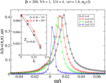
Figure 11: (Color online) $c$-electron spectral function $A_{c}({\boldsymbol{k}}=(\pi,\pi),\omega)$ as a function of the electron-phonon coupling. Inset: QP residue as obtained from fitting the $\beta t=120$ ($\beta t=200$) data to the form of Eq. (18) in the range $30<\tau t<50$ ($30<\tau t<70$), respectively.

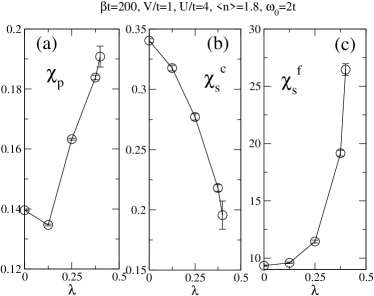
Figure 12: (a) Pair (b) conduction- and (c) $f$-spin susceptibilities as a function of the electron phonon coupling at our lowest temperature, $\beta t=200$.

As expected, Fig. 11 tracks the evolution of $T_{\rm coh}$ – as defined by the peak position in $A_{c}({\boldsymbol{k}}=(\pi,\pi),\omega)$ and the QP residue $Z_{{\boldsymbol{k}}=(\pi,\pi)}$ – as a function of growing electron phonon couplings and at fixed phonon frequency $\omega_{0}=2t$. In the considered electron-phonon coupling range we observe a considerable decrease of this quantity, and the data is consistent with a vanishing $T_{\rm coh}$ at $\lambda\simeq 0.5$. The fact that we cannot account for this large suppression of $T_{\rm coh}$ within the ME approximation highlights the importance of vertex corrections in this parameter range.

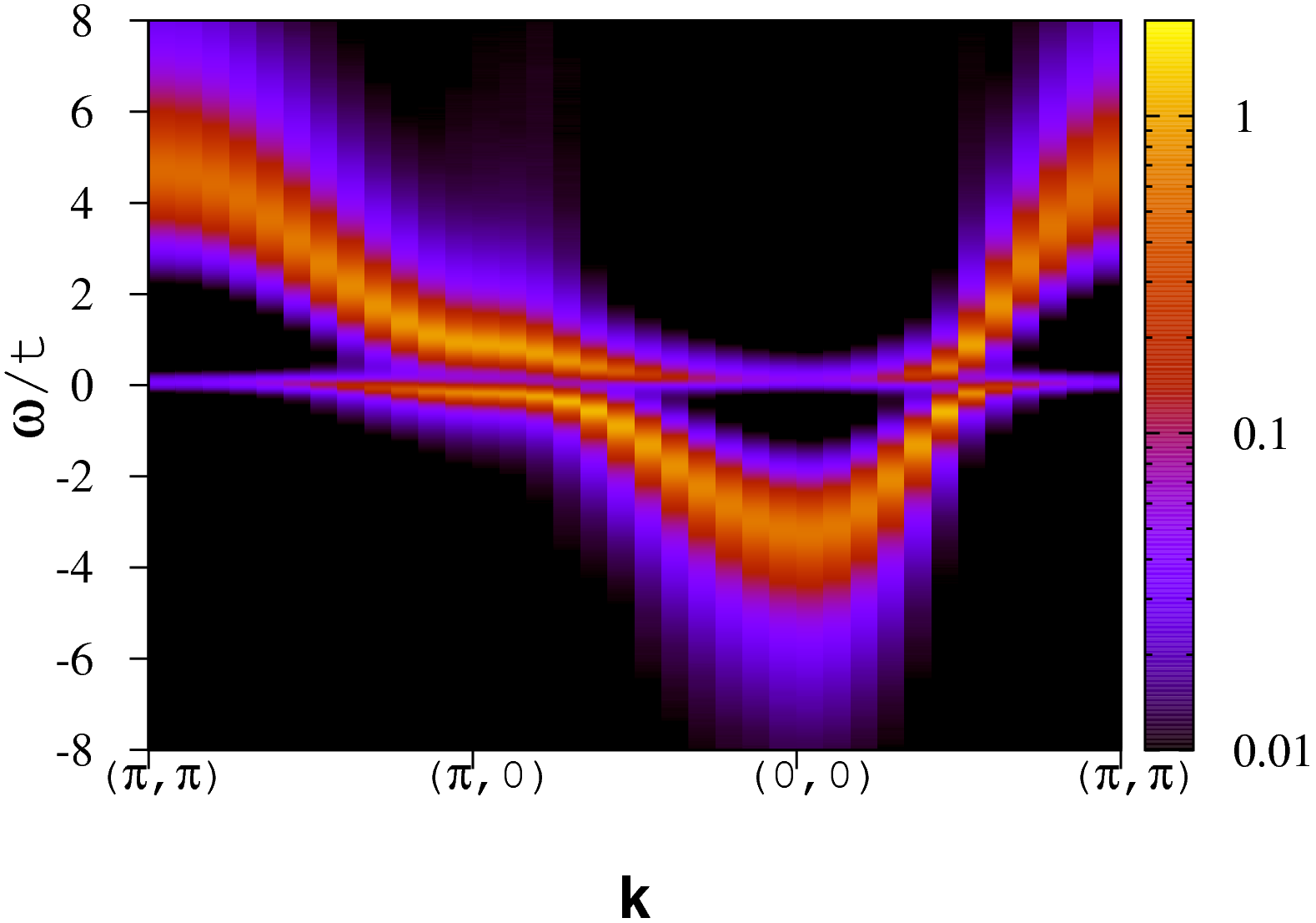
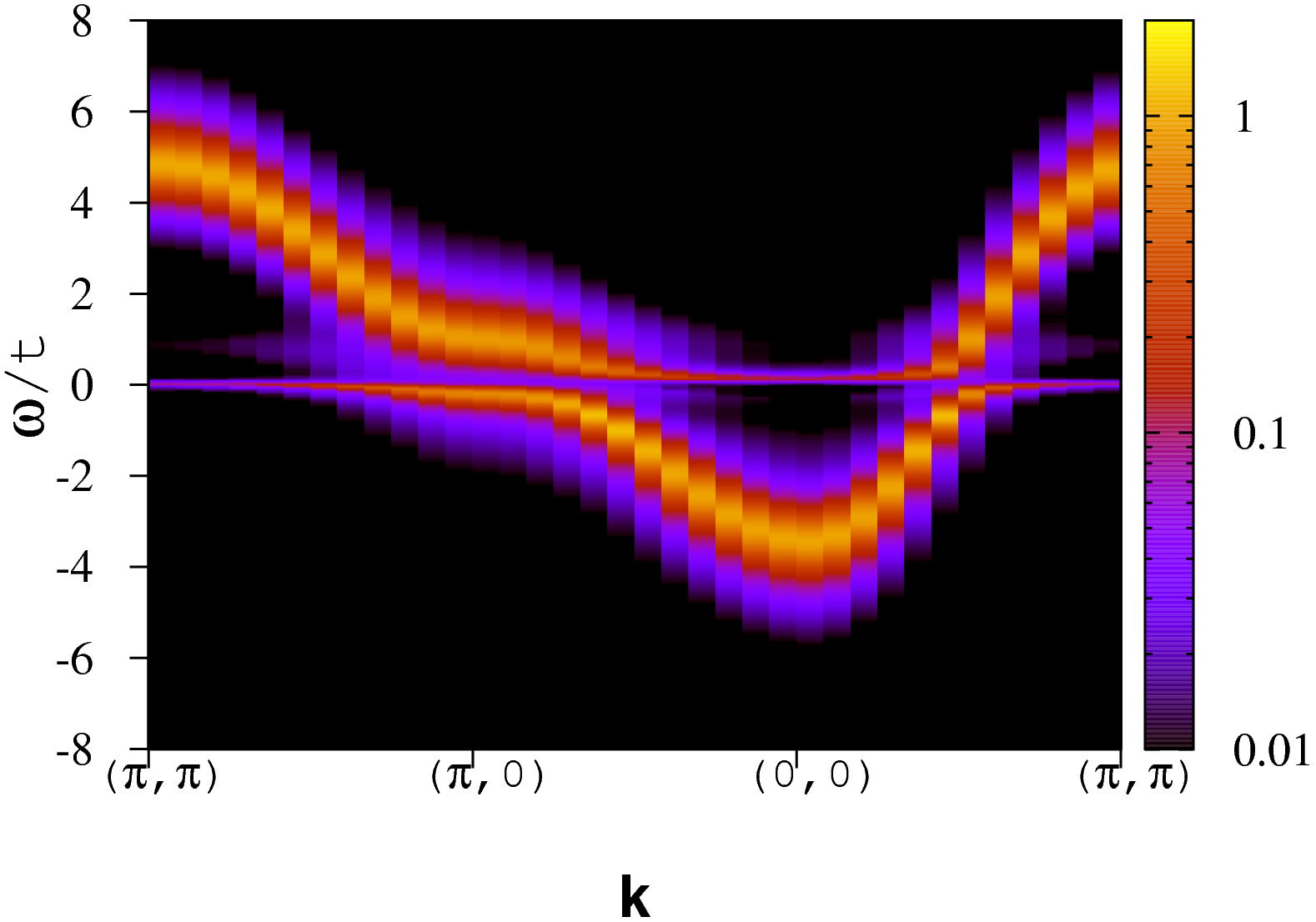
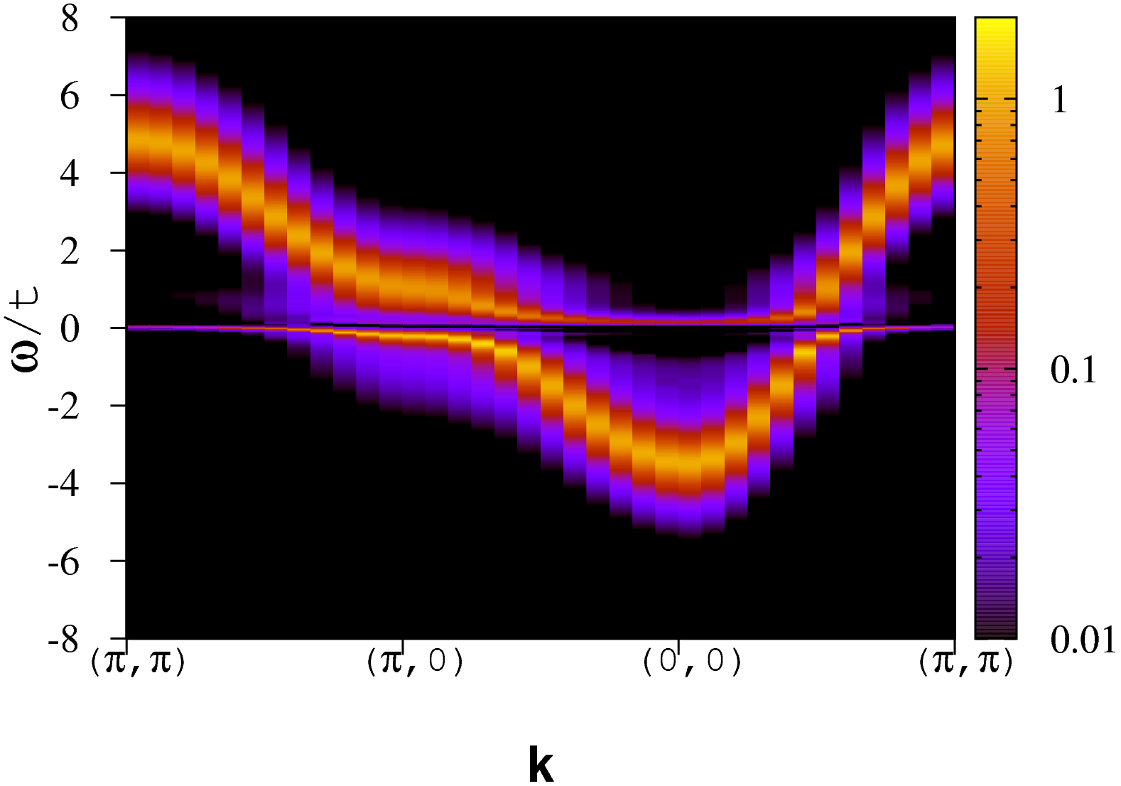
Figure 13: (Color online) $c$-electron single-particle spectral function in the absence of phonons. The models parameters are given by $V/t=1$, $U/t=4$, $\epsilon_{f}=\mu$, and $\langle n\rangle=1.8$. The temperature from top to bottom corresponds to $\beta t=10,20,\text{and }120$.

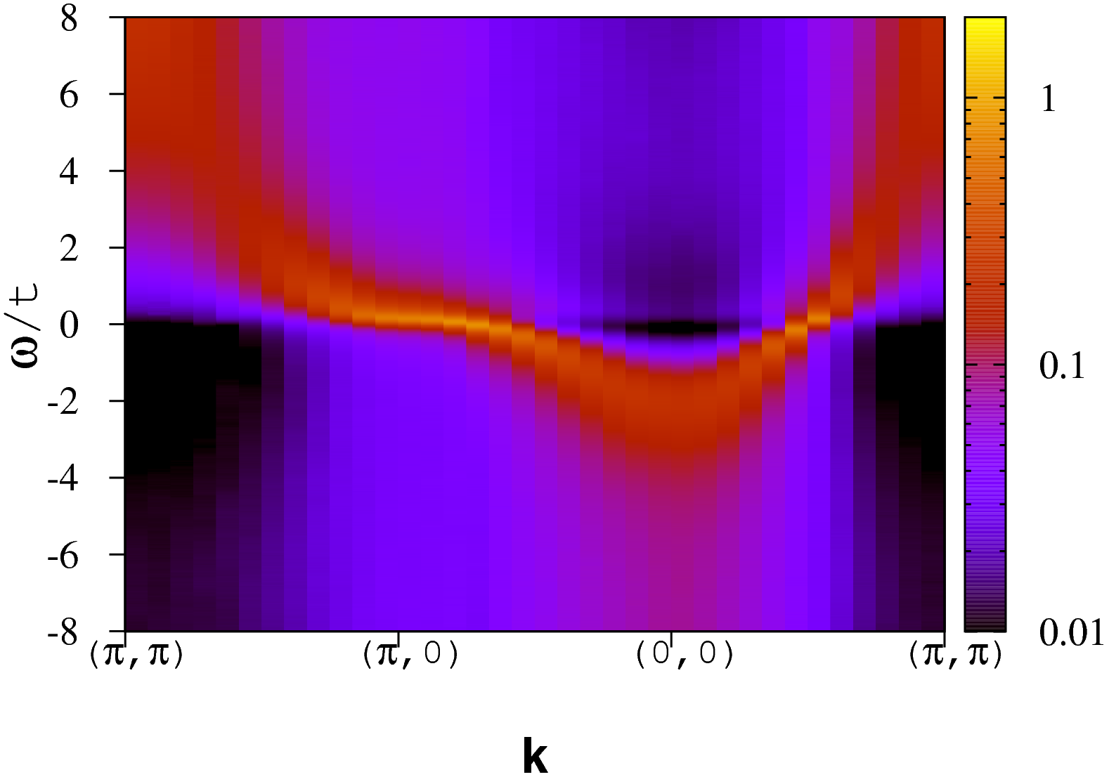
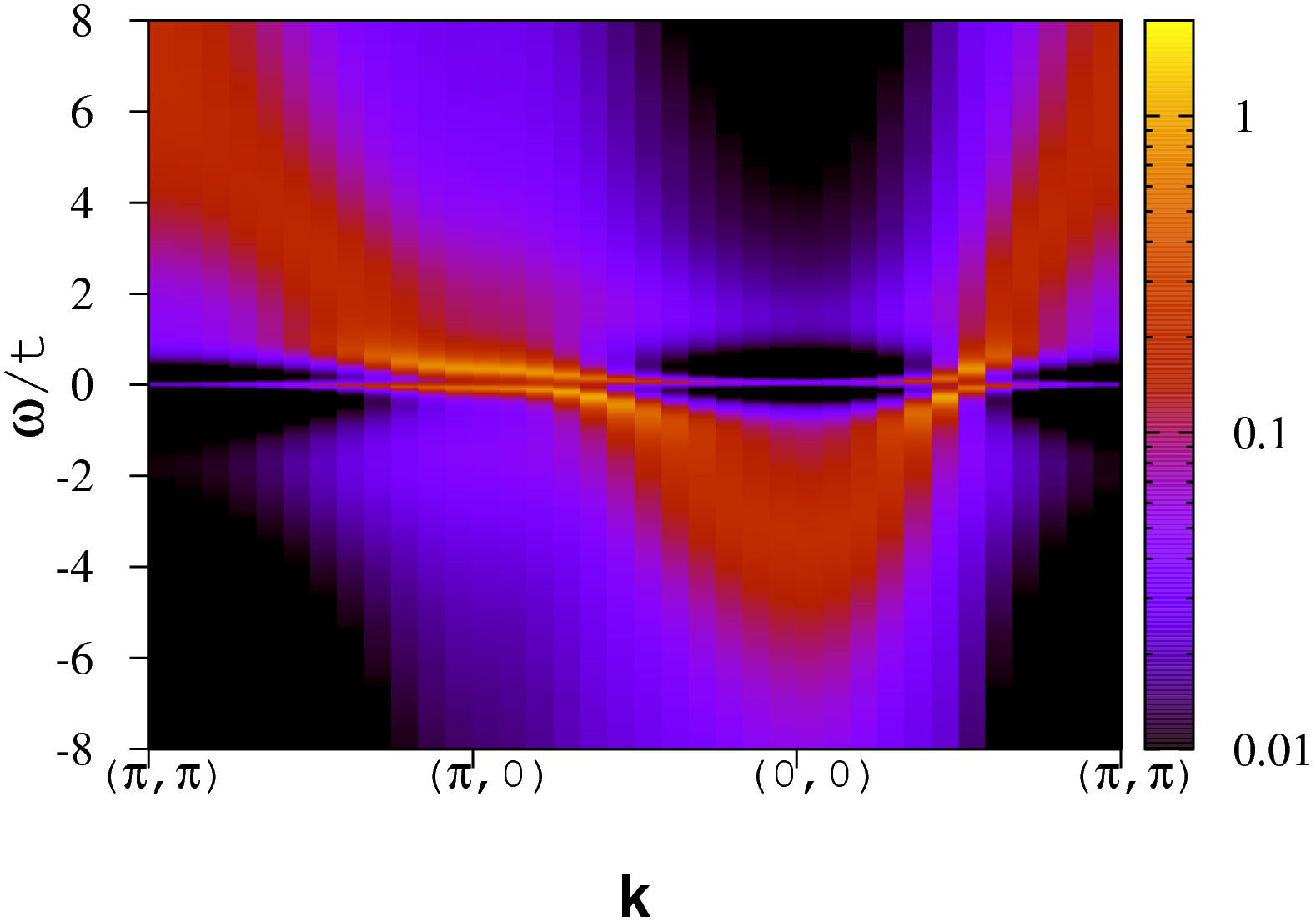
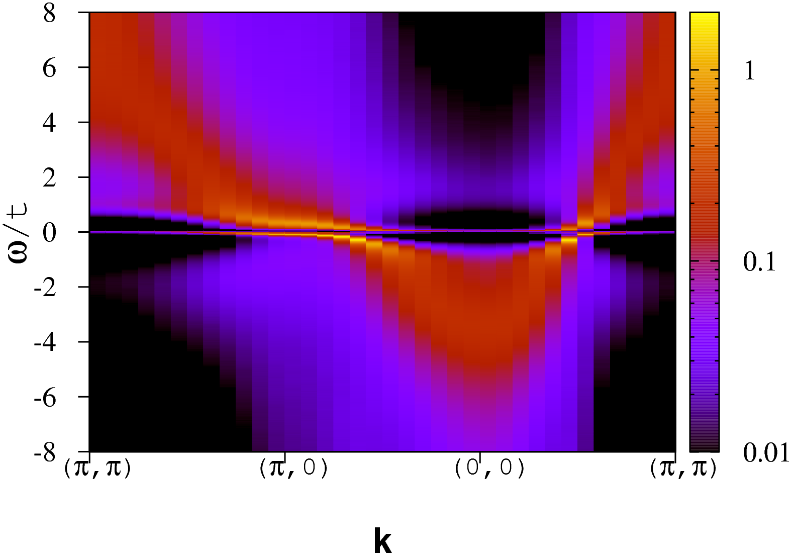
Figure 14: (Color online) Same as in Fig. 13 but in the presence of phonons with $\lambda=0.375$ and $\omega_{0}=2t$.

To confirm that the drop in $T_{\rm coh}$ is driven by electron binding we have computed the local pairing, $\chi_{p}$, and spin susceptibilities, $\chi_{s}^{\alpha}$ on the cluster as defined by

$$\chi_{p} =\int_{0}^{\beta}{\rm d}\tau\langle c^{\dagger}_{\uparrow}(\tau)c^{\dagger}_{\downarrow}(\tau)c_{\downarrow}c_{\uparrow}\rangle,$$ (19)

$$\chi_{s}^{\alpha} =\int_{0}^{\beta}{\rm d}\tau\langle S_{z}^{\alpha}(\tau)S_{z}^{\alpha}\rangle,$$

where $\alpha$ stands for the conduction or $f$-electron in the corresponding impurity problem. Those quantities are plotted in Fig. 12. As shown in Fig. 12(a), after an initial drop, the pair susceptibility grows and tracks the decrease of the coherence temperature. The growth stems from conduction electron binding which originates from the attractive retarded interaction between conduction electrons mediated by a phonon exchange. Regarding a small drop in $\chi_{p}$ at weak electron-phonon coupling, we understand this drop in terms of quasiparticle formation: the bare electron which enters our definition of the singlet $s$-wave pair acquires a smaller overlap with the QP as a function of growing $\lambda$. This dressing of the bare electron reduces the pair susceptibility and initially overcomes the growth of this quantity due to electron binding.

Electron binding into $s$-wave singlets as suggested by Fig. 12(a) lead to a drop of the conduction spin susceptibility. This is clearly seen in Fig. 12(b). Indeed, pairing of conduction electrons competes with the Kondo effect in which conduction electrons form an entangled state with the $f$-electrons thereby screening the magnetic impurities. Therefore, growing values of $\lambda$ are linked to a breakdown of the Kondo singlets and hence a growth of the $f$-spin susceptibility as shown in Fig. 12(c). This behavior should be contrasted with results obtained in complementary studies of the PAM extended by phonon coupling to the $f$-electrons.Ono05 In this case, electron-phonon coupling generates not only pairing between $f$-orbitals but also indirectly via finite mixed valence induces binding of the conduction electrons.

Furthermore, Figs. 13 and 14 compare the temperature dependence of the $c$-electron single-particle spectral functions with and without phonon degrees of freedom. In the absence of the electron phonon interaction, it has been shown Beach08 that signatures of the hybridized bands in the single-particle spectral function emerge below the single-ion Kondo temperature. On the other hand, it is only below the coherence temperature that a well define hybridization gap is visible. As shown in Ref. Beach08, , this hybridization gap leads to a plateau feature in the magnetization curve. The plots in Fig. 13 do not include coupling to the phonon degrees of freedom and point to the gradual formation of the hybridization gap. It is only at the lowest shown temperature, $\beta t=120$, that a clear hybridization gap is apparent. The SB mean-field analysis gives $T_{K}/t\simeq 0.7$ for this parameter set. Hence, for the temperature range considered in Fig. 13 and in the absence of electron-phonon interaction, we always expect signatures of the hybridized band structure when the data is taken below the Kondo temperature.

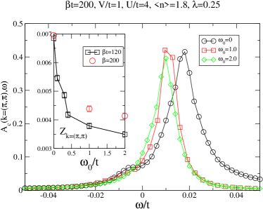
Figure 15: (Color online) Single-particle spectral function of the conduction electrons and QP residue (inset) at fixed electron-phonon coupling, $\lambda=0.25$, and as a function of phonon frequency. The data points at $\omega_{0}=0$ correspond to the case without phonons.

Turning on the electron phonon interaction to $\lambda=0.375$ and setting the phonon frequency to $\omega_{0}=2t$ reduces $T_{\rm coh}$ – as measured by the QP residue (see Fig. 11) – by roughly an order of magnitude. Since one expects the Kondo temperature to track the coherence temperature, a similar reduction of the former quantity is foreseen. Our highest temperature spectral function, $\beta t=10$, in Fig. 14 shows no sign of the hybridization bands thus confirming the substantial reduction of this scale upon inclusion of the electron-phonon coupling. At this temperature, only high energy features and an enhancement of the effective mass by the phonon degrees of freedom is apparent in the data. The Fermi surface of this state accounts solely for the conduction electrons. Upon lowering the temperature, a hybridization gap is restored in the QP band but its width is substantially reduced as compared to the corresponding one in Fig. 13. Only at our lowest considered temperature one can perceive the coherent heavy fermion metallic state with very faint QP peak crossing the Fermi energy in the vicinity of the Brillouin zone corner ${\boldsymbol{k}}=(\pi,\pi)$ thus indicating reconstruction of a large Fermi surface including both the conduction and $f$-electrons.

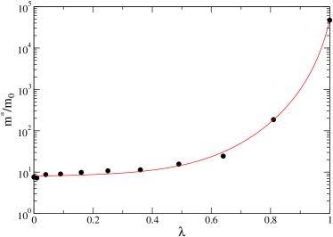
Figure 16: (Color online) QP residue $Z$ as a function of electron-phonon coupling $\lambda$ in the KLM with $J=W/2$, $\omega_{0}=W/2$ while $W=0.2$. The conduction band filling is $n_{c}=0.8$. The red line is a guide to the eye.

We have up to now considered only a fixed phonon frequency and altered the electron phonon coupling. Fig. 15 considers the evolution of $T_{\rm coh}$ at a fixed electron-phonon interaction, $\lambda=0.25$, and as a function of frequency $\omega_{0}/t$. As apparent, there is a rapid convergence to the high-frequency limit. This crossover between the high-frequency and low-frequency behavior compares remarkably well with the energy scale of $T_{\rm K}$ as estimated from the SB mean-field calculations (cf. Table 1).

To capture the low energy behavior of the above transition, we concentrate on the KLM of Eq. (2). This model is an effective low energy model for the PAM in the limit where charge fluctuations on the $f$-sites are negligible. Considering the KLM facilitates the study of the low energy physics in this limit. We have equally used an NRG solver Bulla08 to at best resolve the low energies.

In Fig. 16 we show the variation of the effective mass, $m^{*}\propto 1/Z$, induced by increasing electron-phonon coupling, $\lambda$, while keeping the phonon frequency fixed at $\omega_{0}=W/2$. In analogy to our results for the PAM (see Fig. 11) one observes a divergence of $m^{*}$, or equivalently a vanishing of the coherence temperature.

Next, it is particularly instructive to follow the single particle spectral function, Fig. 17, and corresponding density of states, Fig. 18, as a function of electron phonon coupling. At weak and intermediate electron-phonon couplings, $\lambda<0.8$, essentially the same low energy single particle spectral function is observed but with a renormalized effective mass. Both at $\lambda=0$ and $\lambda=0.25$ the single particle density of states (see Fig. 18) shows a very clear hybridization gap which becomes somewhat smaller as a function of growing electron-phonon coupling thereby reflecting the reduction of the coherence temperature.

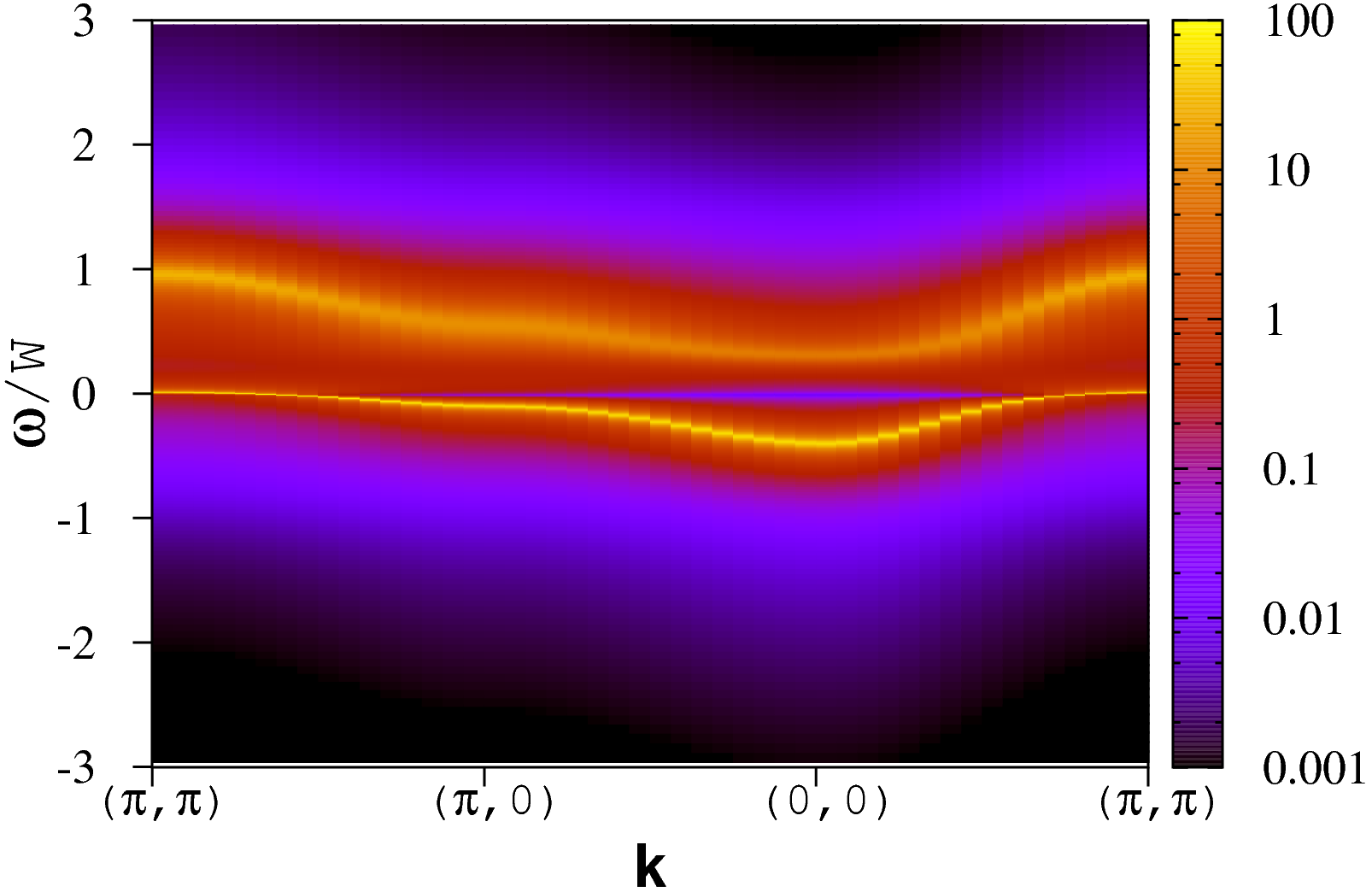
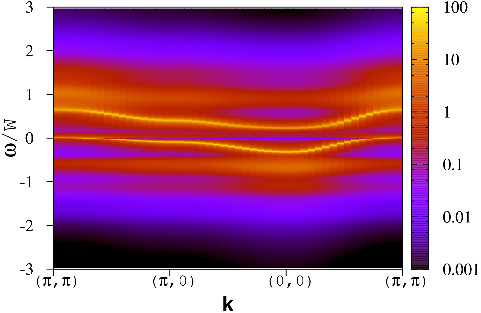
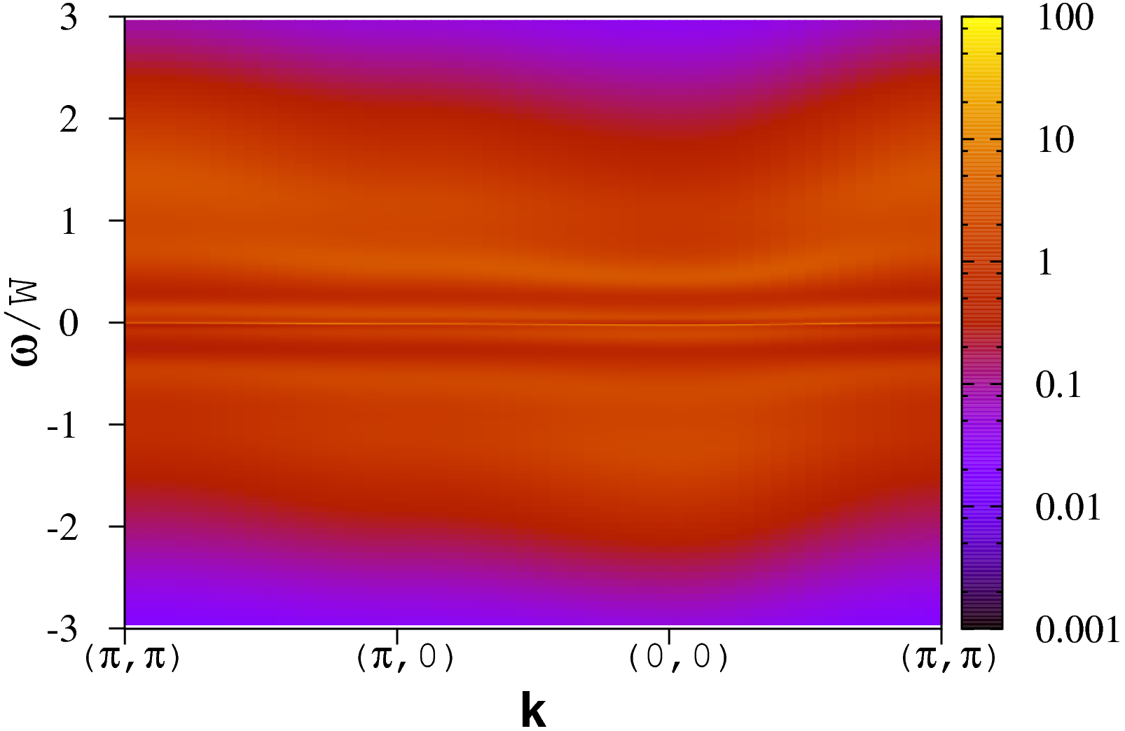
Figure 17: (Color online) Closing hybridization gap on increasing electron-phonon coupling $\lambda$ as seen in the $c$-electron single-particle spectral function $A_{c}({\bf k},\omega)$: $\lambda=0$ (top), $\lambda=0.25$ (middle), and $\lambda=1$ (bottom). Parameters as in Fig. 16.

In contrast, the data set at $\lambda=1$ in Figs. 17 and 18 stands apart. Here we are in the regime where the dynamics of the $f$-spin is frozen as signalized by $\lim_{T\rightarrow 0}T\chi_{s}^{f}>0$ [see Eq. (19)]. In a static mean field approach, this state is captured by the vanishing hybridization matrix element and thereby leads to a total decoupling of the $f$- and $c$-electrons. Following this picture one expects the conduction-electron spectral function to correspond to that of tight-binding electrons coupled to the phonon degrees of freedom thereby producing coherent low energy single particle excitations with enhanced mass. However, this simple picture does not fit the numerical data which shows no sign of a coherent quasiparticle. Hence, an alternative interpretation is required.

The characteristic feature of the state considered here is the frozen dynamics of the $f$-spin which essentially leads to a separation of time scales; the conduction electron propagates in the static magnetic background of the $f$-spins. Since in the DMFT we do not allow for spin ordering, it is very tempting to describe the magnetic background in terms of an $f$-spin which points in a random direction on each site.

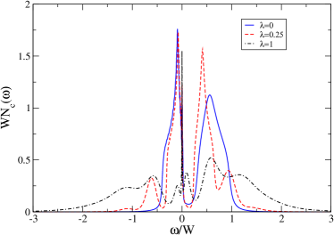
Figure 18: (Color online) Closing hybridization gap on increasing electron-phonon coupling $\lambda$ as seen in the $c$-electron density of states. Parameters as in Fig. 16.

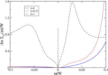
Figure 19: (Color online) Low frequency closeup of the imaginary part of the self-energy as obtained for increasing electron-phonon coupling from the NRG simulations. Parameters as in Fig. 16.

This simple model of disorder, which can be dealt with within a Coherent Potential Approximation (CPA) naturally accounts for the incoherent features of the low energy spectral function seen at $\lambda=1$. The incoherence of the single particle spectral function is clearly seen in the self-energy data of Fig. 19; at $\lambda=1$ and in the low frequency limit, the imaginary part of this quantity remains finite. note A similar argument was used in Ref. Luitz09, to account for the physics of the single-particle spectral function in the local moment regime of the PAM with $s$-wave superconducting BCS conduction electrons.

IV Conclusions

In this paper, we have shown that the low coherence temperature characteristic of heavy fermions compounds leads to the breakdown of the Migdal theorem. In particular, the dominant effect which competes with the formation of the heavy fermion metallic state is conduction electron binding which inhibits Kondo screening of the impurity spins. Since the Kondo temperature is a small scale, already weak electron-phonon coupling leads to a large reduction of the coherence temperature and ultimately to a Kondo breakdown. Our studies were conducted in the local moment regime of the periodic Anderson model and Kondo lattice model in which phonon degrees of freedom predominantly couple to the conduction electrons. Hence, we can conjecture that heavy fermion materials in the local moment regime should show no phonon anomalies since this would imply a large electron-phonon interaction which as we have shown leads to the breakdown of the heavy fermion metallic state. Moreover, since the electron-phonon interaction considerably lowers the coherence and Kondo scales, it implicitly enhances the importance of magnetic instabilities driven by the Ruderman-Kittel-Kasuya-Yosida (RKKY) interaction between the local moments. It also leads to pairing hence potentially favoring superconductivity. The delicate interplay between those phonon driven instabilities can only be understood within the framework of cluster methods and is the goal of future investigations.

*

Appendix A Slave-boson technique and the Migdal-Eliashberg approximation

In the SB method one enlarges the Hilbert space by introducing a set of four auxiliary bosonic fields $e_{i}$, $p_{i\pm\sigma}$, and $d_{i}$ corresponding to empty, singly and doubly occupied impurity sites, respectively, such that the $f$-electron operators are replaced by $f_{i\sigma}\to{\tilde{f}}_{i\sigma}z_{i\sigma}$, with

$$z_{i\sigma}=\frac{e_{i}^{{\dagger}}p_{i\sigma}+p_{i-\sigma}^{{\dagger}}d_{i}}{\sqrt{1-d^{{\dagger}}_{i}d_{i}-p_{i\sigma}^{{\dagger}}p_{i\sigma}}\sqrt{1-e^{{\dagger}}_{i}e_{i}-p_{i-\sigma}^{{\dagger}}p_{i-\sigma}}}.$$ (20)

However, such enlargement of the Hilbert space introduces unphysical states which should be eliminated so as to recover the original Hilbert space. Therefore, the SB operators have to fulfill the following constraints at each site,

$$e_{i}^{{\dagger}}e_{i}+d_{i}^{{\dagger}}d_{i}+\sum_{\sigma}p_{i\sigma}^{{\dagger}}p_{i\sigma} =1,$$ (21)

$$d_{i}^{{\dagger}}d_{i}+p_{i\sigma}^{{\dagger}}p_{i\sigma} ={\tilde{f}}_{i\sigma}^{{\dagger}}{\tilde{f}}_{i\sigma}.$$

The constraints enforced by time-dependent Lagrange multipliers $\lambda_{i}^{(1)}$ and $\lambda_{i\sigma}^{(2)}$ are conveniently handled in a path integral formulation. Indeed, the SB partition function of the periodic Anderson model may be written down as a functional integral over coherent states of Fermi and Bose fields,

$$Z_{SB}=\int D[e,p_{\pm\sigma},d]D[c,{\tilde{f}}]D[\lambda^{(1)},\lambda^{(2)}_{\pm\sigma}]e^{-(\mathcal{S}_{B}+\mathcal{S}_{F})},$$ (22)

with the bosonic,

$$\mathcal{S}_{B} =\int\limits_{0}^{\beta}d\tau\sum_{i}\Bigl{\{}d_{i}^{{\dagger}}\bigl{(}\partial_{\tau}+\lambda_{i}^{(1)}-\sum_{\sigma}\lambda_{i\sigma}^{(2)}+U\bigr{)}d_{i}-\lambda_{i}^{(1)}$$ (23)

$$+e_{i}^{{\dagger}}\big{(}\partial_{\tau}+\lambda_{i}^{(1)}\bigr{)}e_{i}+\sum_{\sigma}p_{i\sigma}^{{\dagger}}\bigl{(}\partial_{\tau}+\lambda_{i}^{(1)}-\lambda_{i\sigma}^{(2)}\bigr{)}p_{i\sigma}\Bigr{\}},$$

and fermionic,

$$\mathcal{S}_{F}=\int\limits_{0}^{\beta}d\tau\Bigl{\{}H_{0}+\sum_{i\sigma}{\tilde{f}}_{i\sigma}^{{\dagger}}\bigl{(}\partial_{\tau}+{\tilde{\epsilon}_{f}}\bigr{)}{\tilde{f}}_{i\sigma}+V\sum_{i\sigma}c_{i}^{{\dagger}}z_{i\sigma}{\tilde{f}}_{i\sigma}\Bigr{\}},$$ (24)

actions. In Eq. (24), ${\tilde{\epsilon}_{f}}=\epsilon_{f}+\lambda_{i\sigma}^{(2)}-U/2-\mu$ is a renormalized $f$-level energy. Next, we assume the translation and spin SU(2) invariance and apply the saddle-point approximation in which one replaces all the Bose fields and Lagrange multipliers by their time-independent averages, i.e., $p\equiv\langle p_{i\sigma}^{{\dagger}}(\tau)\rangle=\langle p_{i\sigma}(\tau)\rangle$, and so on. The site-normalized SB mean-field free energy becomes,

$$F_{SB} =-\frac{2}{\beta N}\sum_{{\boldsymbol{k}},n=\pm}\ln\bigl{(}1+e^{-\beta E_{n}({\boldsymbol{k}})}\bigr{)}+\mu\langle n\rangle$$ (25)

$$+\lambda^{(1)}(e^{2}+2p^{2}+d^{2}-1)-2\lambda^{(2)}(p^{2}+d^{2})+Ud^{2},$$

with,

$$E_{\pm}({\boldsymbol{k}})=\frac{1}{2}\Bigl{[}{\tilde{\epsilon}_{f}}+\epsilon({\boldsymbol{k}})\pm\sqrt{[{\tilde{\epsilon}_{f}}-\epsilon({\boldsymbol{k}})]^{2}+4(zV)^{2}}\Bigr{]},$$ (26)

being the energies of the hybridized bands. The equilibrium values of the classical field amplitudes as well as of the chemical potential $\mu$ are determined by the minimization $F_{SB}$ with respect to these parameters:

$$\frac{\partial F_{SB}}{\partial\lambda^{(1)}} =e^{2}+2p^{2}+d^{2}-1=0,$$ (27)

$$\frac{\partial F_{SB}}{\partial\lambda^{(2)}} =\langle{\tilde{f}}^{{\dagger}}{\tilde{f}}\rangle-\bigl{(}p^{2}+d^{2}\bigr{)}=0,$$

$$\frac{\partial F_{SB}}{\partial e} =\lambda^{(1)}e+V\frac{\partial z}{\partial e}\chi_{cf}=0,$$

$$\frac{\partial F_{SB}}{\partial d} =\bigl{(}\lambda^{(1)}-2\lambda^{(2)}+U\bigr{)}d+V\frac{\partial z}{\partial d}\chi_{cf}=0,$$

$$\frac{\partial F_{SB}}{\partial p} =\bigl{(}\lambda^{(1)}-\lambda^{(2)}\bigr{)}p+V\frac{\partial z}{\partial p}\chi_{cf}=0,$$

$$\frac{\partial F_{SB}}{\partial\mu} =\langle n\rangle-2\Bigl{(}\langle c^{{\dagger}}c\rangle+\langle{\tilde{f}}^{{\dagger}}{\tilde{f}}\rangle\Bigr{)},$$

where we have defined average bond hopping $\chi_{cf}=\langle c^{{\dagger}}{\tilde{f}}\rangle+h.c$. The expectation values $\langle\alpha^{{\dagger}}\beta\rangle$ with $\alpha\equiv\{c,{\tilde{f}}\}$ are obtained from the local one-particle Green’s functions which allows one to combine the SB approach with the ME approximation to account for the phonon degrees of freedom. The self-consistent evaluation of the diagram of Fig. 1 amounts to solving:

$$\Sigma_{cc}(i\omega_{m})=\frac{g^{2}\omega_{0}}{2k}\frac{1}{\beta N}\sum_{{\boldsymbol{k}},i\Omega_{m}}D^{0}(i\Omega_{m})G_{cc}({\boldsymbol{k}},i\omega_{m}-i\Omega_{m}),$$ (28)

with

$${\boldsymbol{\cal G}}({\boldsymbol{k}},i\omega_{m}) \equiv\left(\begin{array}[]{cc}G_{cc}({\boldsymbol{k}},i\omega_{m})&G_{cf}({\boldsymbol{k}},i\omega_{m})\\ G_{fc}({\boldsymbol{k}},i\omega_{m})&G_{ff}({\boldsymbol{k}},i\omega_{m})\end{array}\right)$$ (29)

$$=\frac{1}{{\boldsymbol{\cal G}}^{-1}_{0}({\boldsymbol{k}},i\omega_{m})-\left(\begin{array}[]{cc}\Sigma_{cc}(i\omega_{m})&0\\ 0&0\end{array}\right)}.$$

Here $D^{0}(i\Omega_{m})=\frac{1}{\omega_{0}+i\Omega_{m}}+\frac{1}{\omega_{0}-i\Omega_{m}}$ is the bare phonon propagator, $\omega_{m}$ ($\Omega_{m}$) are fermionic (bosonic) Matsubara frequencies, respectively, and ${\boldsymbol{\cal G}}_{0}({\boldsymbol{k}},i\omega_{m})$ is the $2\times 2$ Green function matrix as obtained from the SB mean-field Hamiltonian at the given iteration step. Since at a given iteration we do not have at hand the pole structure of $G_{cc}({\boldsymbol{k}},i\omega_{m})$ in the complex frequency plane, we solve the above equation numerically for real frequencies. Namely, we use the spectral representation of the Green’s function:

$$G_{cc}({\boldsymbol{k}},i\omega_{m})=\int{\rm d}\omega^{\prime}\frac{A_{c}({\boldsymbol{k}},\omega^{\prime})}{i\omega_{m}-\omega^{\prime}},$$ (30)

where $A_{c}({\boldsymbol{k}},\omega^{\prime})=-\frac{1}{\pi}{\rm Im}G_{cc}^{{\rm ret}}({\boldsymbol{k}},\omega^{\prime})$, and perform summation over bosonic Matsubara frequencies so that the self-energy reads:

$$\Sigma_{cc}(i\omega_{m}) =\frac{g^{2}}{2k}\omega_{0}\int{\rm d}\omega^{\prime}N_{c}(\omega^{\prime})$$

$$\times\left\{\frac{n_{b}(\omega_{0})+1-n_{f}(\omega^{\prime})}{-\omega^{\prime}-\omega_{0}+i\omega_{m}}+\frac{n_{b}(\omega_{0})+n_{f}(\omega^{\prime})}{-\omega^{\prime}+\omega_{0}+i\omega_{m}}\right\},$$ (31)

where $N_{c}(\omega^{\prime})\equiv\frac{1}{N}\sum_{{\boldsymbol{k}}}A_{c}({\boldsymbol{k}},\omega^{\prime})$ is $c$-electron density of states, while $n_{f}[\epsilon(\boldsymbol{k})]=\frac{1}{e^{\beta\epsilon(\boldsymbol{k})}+1}$ and $n_{b}(\omega_{0})=\frac{1}{e^{\beta\omega_{0}}-1}$ are the Fermi function and Bose-Einstein distribution, respectively. Hence, at a given iteration step at which $N_{c}(\omega)$ is known we compute with the above equation the self-energy on the real frequency axis ($i\omega_{m}\rightarrow\omega+i\delta$) and thereby recompute the single-particle Green’s function and corresponding $N_{c}(\omega)$ until convergence of $\Sigma_{cc}(i\omega_{m})$ is reached. This in turn allows one to determine the local Green’s functions which satisfy the usual Dyson equation (29). Explicitly one finds:

$$G_{cc}({\boldsymbol{k}},i\omega_{m}) =\frac{1}{i\omega_{m}-\epsilon({\boldsymbol{k}})-\Sigma_{cc}^{eff}(i\omega_{m})},$$ (32)

$$G_{ff}({\boldsymbol{k}},i\omega_{m}) =\frac{1}{i\omega_{m}-{\tilde{\epsilon}_{f}}-\Sigma_{ff}^{eff}({\boldsymbol{k}},i\omega_{m})},$$

$$G_{cf}({\boldsymbol{k}},i\omega_{m}) =\frac{zV}{(zV)^{2}-\Sigma_{cf}^{eff}({\boldsymbol{k}},i\omega_{m})},$$

where we have defined the effective self-energies:

$$\Sigma_{cc}^{eff}(i\omega_{m}) =\Sigma_{cc}(i\omega_{m})+\frac{(zV)^{2}}{i\omega_{m}-{\tilde{\epsilon}_{f}}},$$ (33)

$$\Sigma_{ff}^{eff}({\boldsymbol{k}},i\omega_{m}) =\frac{(zV)^{2}}{i\omega_{m}-\epsilon({\boldsymbol{k}})-\Sigma_{cc}(i\omega_{m})},$$

$$\Sigma_{cf}^{eff}({\boldsymbol{k}},i\omega_{m}) =[i\omega_{m}-\epsilon({\boldsymbol{k}})-\Sigma_{cc}(i\omega_{m})](i\omega_{m}-{\tilde{\epsilon}_{f}}).$$

Finally, the expectation values $\langle\alpha^{{\dagger}}\beta\rangle$ entering the SB saddle-point equations are obtained by performing the Fourier transformations:

$$\langle\alpha^{{\dagger}}(\tau)\beta\rangle=-\frac{1}{\beta N}\sum_{{\boldsymbol{k}},\omega_{m}}e^{-i\omega_{m}\tau}G_{\alpha\beta}({\boldsymbol{k}},i\omega_{m}),$$ (34)

and the whole process is iterated until the SB mean-field equations (27) are fulfilled.

References

- (1) H. v. Löhneysen, A. Rosch, M. Vojta, and P. Wölfle, Rev. Mod. Phys. 79, 1015 (2007).
- (2) T. M. Rice and K. Ueda, Phys. Rev. B 34, 6420 (1986).
- (3) S. Burdin, A. Georges, and D. R. Grempel, Phys. Rev. Lett. 85, 1048 (2000).
- (4) T. Pruschke, R. Bulla, and M. Jarrell, Phys. Rev. B 61, 12799 (2000).
- (5) F. F. Assaad, Phys. Rev. B 70, 020402(R) (2004).
- (6) A. Migdal, JETP 34, 996 (1958).
- (7) K. Mitsumoto and Y. Ono, Physica C 426, 330 (2005); ibid. J. Magn. Magn. Mater. 310, 419 (2007).
- (8) G. Kotliar and A. E. Ruckenstein, Phys. Rev. Lett. 57, 1362 (1986).
- (9) G. Eliashberg, JETP 11, 696 (1960).
- (10) S. Engelsberg and J. R. Schrieffer, Phys. Rev. 131, 993 (1963).
- (11) A. N. Rubtsov, V. V. Savkin, and A. I. Lichtenstein, Phys. Rev. B 72, 035122 (2005).
- (12) F. F. Assaad and T. C. Lang, Phys. Rev. B 76, 035116 (2007).
- (13) F. F. Assaad, Phys. Rev. B 78, 155124 (2008).
- (14) R. Bulla, T. A. Costi, and T. Pruschke, Rev. Mod. Phys. 80, 395 (2008).
- (15) M. Raczkowski, R. Frésard, and A. M. Oleś, Phys. Rev. B 73, 174525 (2006); Europhys. Lett. 76, 128 (2006).
- (16) R. Frésard and G. Kotliar, Phys. Rev. B 56, 12909 (1997).
- (17) A. M. Reynolds, D. M. Edwards, and A. C. Hewson, J. Phys.: Condens. Matter 4, 7589 (1992); V. Dorin and P. Schlottmann, Phys. Rev. B 46, 10800 (1992); B. Möller and P. Wölfle, ibid. 48, 10320 (1993); R. Doradziński and J. Spałek, ibid. 56, R14239 (1997); P. D. Sacramento, J. Aparício, and G. S. Nunes, J. Phys.: Condens. Matter 22, 065702 (2010).
- (18) S. Burdin and V. Zlatić, Phys. Rev. B 79, 115139 (2009).
- (19) M. Brunner, F. F. Assaad, and A. Muramatsu, Phys. Rev. B 62, 15 480 (2000).
- (20) A. S. Mishchenko, N. V. Prokof’ev, and B. V. Svistunov, Phys. Rev. B 64, 033101 (2001).
- (21) A. Lüscher, A. Läuchli, W. Zheng, and O. P. Sushkov, Phys. Rev. B 73, 155118 (2006).
- (22) G. Martinez and P. Horsch, Phys. Rev. B 44, 317 (1991).
- (23) A. Ramšak and P. Horsch, Phys. Rev. B 57, 4308 (1998).
- (24) C. Slezak, A. Macridin, G. A. Sawatzky, M. Jarrell, and T. A. Maier, Phys. Rev. B 73, 205122 (2006).
- (25) O. Gunnarsson and O. Rösch, Phys. Rev. B 73, 174521 (2006).
- (26) J. van den Brink, P. Horsch, and A. M. Oleś, Phys. Rev. Lett. 85, 5174 (2000).
- (27) K. S. D. Beach, arXiv:cond-mat/0403055 (unpublished).
- (28) K. S. D. Beach and F. F. Assaad, Phys. Rev. B 77, 205123 (2008).
- (29) Strictly speaking, at the effective mass is very large but finite (see Fig. 16). One can check that on a scale set by the inverse effective mass the imaginary part of the self energy vanishes.
- (30) D. Luitz and F. F. Assaad, Phys. Rev. B81, 024509 (2010).