Outflows and Massive Stars in the protocluster IRAS 05358+3543

Abstract

We present new near-IR $\textrm{H}_{2}$, CO J=2-1, and CO J = 3-2 observations to study outflows in the massive star forming region IRAS 05358+3543. The Canada-France-Hawaii Telescope $\textrm{H}_{2}$ images and James Clerk Maxwell Telescope CO data cubes of the IRAS 05358 region reveal several new outflows, most of which emerge from the dense cluster of sub-mm cores associated with the Sh 2-233IR NE cluster to the northeast of IRAS 05358. We used Apache Point Observatory (APO) JHK spectra to determine line of sight velocities of the outflowing material. Analysis of archival VLA cm continuum data and previously published VLBI observations reveal a massive star binary as a probable source of one or two of the outflows. We have identified probable sources for 6 outflows and candidate counterflows for 7 out of a total of 11 seen to be originating from the IRAS 05358 clusters. We classify the clumps within Sh 2-233IR NE as an early protocluster and Sh 2-233IR SW as a young cluster, and conclude that the outflow energy injection rate approximately matches the turbulent decay rate in Sh 2-233IR NE.

1 Introduction

Collimated, bipolar outflows accompany the birth of young stars from the earliest stages of star formation to the end of their accretion phase (e.g. Reipurth & Bally 2001). While the birth of isolated low-mass stars is becoming well understood, the formation of massive stars ($>10M_{\odot}$) and clusters remains a topic of intense study. Observations show that moderate to high-mass stars tend to form in dense clusters (Lada & Lada 2003). In a clustered environment, the dynamics of the gas and stars can profoundly impact both accretion and mass-loss processes. Feedback from these massive clusters may play a significant role in momentum injection and turbulence driving in the interstellar medium.

Outflows from massive stars are less studied than those from low mass stars largely because massive stars accrete most of their mass while deeply embedded. Therefore, unlike low mass young stars that are accessible in the optical, massive stellar outflows can only be seen at infrared and longer wavelengths. Direct evidence for jets from massive young stellar objects (YSOs) from $\textrm{H}_{2}$ or optical emission is generally lacking (e.g. Alvarez & Hoare 2005; Kumar et al. 2002; Wang et al. 2003), although there is evidence that massive stars are the sources of collimated molecular outflows from millimeter observations (e.g. Beuther et al. 2002b). Outflows from massive stars may allow accretion to continue after their radiation pressure would otherwise halt accretion in a spherically symmetric system (Krumholz et al. 2009). They therefore represent a crucial component in understanding how stars above $\sim$10 $M_{\odot}$ can form.

IRAS 05358 is a double cluster of embedded infrared sources located at a distance of 1.8 kpc in the Auriga molecular cloud complex (Heyer et al. 1996) associated with the HII regions Sh-2 231 through 235 at Galactic coordinates around $l,~{}b$ = 173.48,+2.45 in the Perseus arm. Sh 2-233IR NE is the collection of highly obscured and mm-bright sources slightly northeast of Sh 2-233IR SW, which is the location of the IRAS 05358+3543 point source and the optical emission nebula (see Figure 1). The IRAS source is probably a blend of the three brightest infrared objects in the MSX A-band and MIPS 24 $\mu m$ images, which are located at Sh 2-233IR NE, IR 41, and IR 6. For the purpose of this paper,the whole complex including both sources is referred toas IRAS 05358, and otherwise refer to individual objects specifically.

Early observations revealed the presence of OH (Wouterloot et al. 1993), $\textrm{H}_{2}\textrm{O}$ (Scalise et al. 1989; Henning et al. 1992), and methanol (Menten 1991) masers about an arcminute northeast of the IRAS source, indicating that massive stars are likely present at that location. Near infrared observations revealed the presence of two embedded clusters (Porras et al. 2000; Jiang et al. 2001) labeled Sh 2-233IR SW for the southwestern cluster associated with the IRAS source, and Sh 2-233IR NE for the northeastern cluster located near the OH, $\textrm{H}_{2}\textrm{O}$, and CH₃OH masers. Stars identified in Porras et al. (2000) are referred to by the designation “IR (number)” corresponding to the catalog number in that paper. Porras et al. (2000) also included scanning Fabry-Perot velocity measurements of the inner $\sim 1$′. CO observations revealed broad line wings indicative of a molecular outflow (Casoli et al. 1986; Shepherd & Churchwell 1996). Kumar et al. (2002) and Khanzadyan et al. (2004) presented narrow band images of 2.12 $\mu m$ $\textrm{H}_{2}$ emission that reveled the presence of multiple outflows. Interferometric imaging of CO and SiO confirmed the presence of at least three flows emerging from the northeast cluster centered on the masers (Beuther et al. 2002a) having a total mass of about 20 $M_{\odot}$. Beuther et al. (2002a) also presented MAMBO 1.2 mm maps and a mass estimate of 610 $M_{\odot}$ for the whole region. Williams et al. (2004) presented SCUBA maps and mass estimates of the clusters of 195/126$M_{\odot}$ for Sh 2-233IR NE and 24/12 $M_{\odot}$ for Sh 2-233IR SW (850 $\mu m$/450 $\mu m$). Zinchenko et al. (1997) measured the dense gas properties using the NH₃ (1,1) and (2,2) lines. They measure a mean density $n\approx 10^{3.60}$ $\textrm{cm}^{-3}$, temperature 26.5K, and a mass of 600 $M_{\odot}$. The total luminosity of the two clusters is about 6300 $L_{\odot}$, indicating that the region is giving birth to massive stars (Porras et al. 2000).

Millimeter wavelength interferometry with arcsecond angular resolution has revealed a compact cluster of deeply embedded sources centered on the $\textrm{H}_{2}\textrm{O}$ and methanol maser position (Beuther et al. 2002a, 2007; Leurini et al. 2007). Beuther et al. (2002a) identified 3 mm continuum cores, labeled mm1-mm3 (shown in Figure 2). Beuther et al. (2007) resolved these cores into smaller objects. Source mm1a is associated with a cm continuum point source and will be discussed in detail below.

IRAS 05358 has previously been observed at low spatial resolution in the J=2-1 and J=3-2 transitions with the Kosma 3m telescope (Mao & Zeng 2004). While the general presence of outflows was recognized and a total mass estimated, the specific outflows were not resolved. Beuther et al. (2002a) observed the CO J=6-5, J=2-1, and J=1-0 transitions at moderate resolution in the inner few arcminutes. Thomas & Fuller (2008) observed C¹⁷O in the J=2-1 and J=3-2 transitions with a single pointing using the JCMT.

2 Observations

A collection of data acquired by the authors and from publicly available archives is presented. An overview of the data is presented in figure 1. The goal was to develop a complete picture of the outflows in IRAS 05358 and their probable sources. CO data were acquired to estimate the total outflowing mass and to identify outflowing molecular material unassociated with $\textrm{H}_{2}$ shocks. Archival Spitzer IRAC and MIPS 24 $\mu m$ data were used to identify probable YSOs as candidate outflow sources. Near-infrared spectra were acquired primarily to determine $\textrm{H}_{2}$ kinematics and develop a 3D picture of the region. Optical spectra were acquired to attempt to identify stellar types in the unobscured Sh 2-233IR SW region. Finally, archival VLA data were used to acquire better constraints on the position and physical properties of the known ultracompact HII (UCHII) region, and to detect or set limits on other UCHIIs.

2.1 Sub-millimeter Observations

The 345 GHz J = 3-2 rotational transition of CO was observed with the James Clerk Maxwell Telescope (JCMT) on 4 January, 2008 with the 16 element (14 functional) HARP-B heterodyne focal plane array. Two 12′ $\times$ 10′  raster scans in R.A. and Dec. were taken with orthogonal orientations to assure complete coverage in the region of interest; this resulted in a useable field 11.7′ $\times$ 11.3′ with higher noise along the edges. The beam size at 345 GHz is about 15″.

Observations were conducted during grade 3 conditions with the 225 GHz zenith optical depth of the atmosphere $\tau\sim 0.1$. A channel width of 488 kHz corresponding to 0.423 km s^-1 was used. The maps required a total of 1 hour to acquire and resulted in an effective integration time of 4.6 seconds per pixel (there are 12,000 $6\times 6\arcsec$ pixels in the final grid), resulting in a noise per pixel of 0.36 K km s^-1.

The optical depth and telescope efficiency corrections were applied by the JCMT pipeline to convert the recorded antenna temperatures to the corrected antenna . An additional main-beam correction has been applied,

$$T_{mb}=\frac{T_{A}*}{\eta_{mb}}$$

where $\eta_{mb}$ was measured by observing Mars to be $\approx 0.60$ at 345 GHz. Emission in the sidelobes is expected to be small at the outflow velocities.

On September 25 and November 15, 2008 the CO, ¹³CO, and C¹⁸O J=2-1 transitions were observed in the central 3′ of IRAS 05358. The beamsize at 220 GHz is about 23″. The sideband configuration used also includes the SO $5_{6}-4_{5}$ and ¹³CS 5-4 transitions. Conditions during these observations were grade 5 ($\tau\sim 0.24-0.28$) and therefore too poor to use the HARP instrument, but acceptable for the A3 detector.

Data reduction used the Starlink package following the standard routines recommended by the JCMT support scientists . The CO 3-2 data cube was extracted over a velocity range from –50 to 10 km s^-1 LSR and spectral baselines were fit over the velocity range –50 to –40 and 0 to 10 km s^-1 and subtracted. The data were re-gridded into 6″  pixels and 2 pixel Gaussian smoothing was used to fill in the gaps left by the two bad detectors in the 4 $\times$4 array. The data cube was cropped to remove undersampled edges which have high noise and bad baselines. The beam efficiency was 0.68 at 230 GHz.

The A3 data cubes were extracted over the velocity range –60 to 20 km s^-1 and baselines were calculated over –60 to –40 and 0 to 20 km s^-1. The data was gridded into 10″ pixels with 2 pixel gaussian smoothing to reduce sub-resolution noise variations.

2.2 Spitzer

Spitzer IRAC bands 1 to 4 and MIPS band 1 data were retrieved from the Spitzer Science Center archive. Qiu et al. (2008) acquired the data as part of a study of many high-mass star forming regions; they identified YSO candidates based on IRAC colors. The version 18 post-BCD data products were used to produce images and photometric catalog from Qiu et al. (2008), which was made from a more carefully-reduced data set, was used for SED analysis.

2.3 Near-IR images

Near-infrared data were acquired using the Wide-field Infrared Camera (WIRCam) on the Canada-France-Hawaii Telescope (CFHT) on Mauna Kea. The field of view is 20′$\times$20′  and pixel scale 0.3″. Data were acquired on November 18, 19 and December 20, 2005. The seeing was 0.5-0.7″ during the observations. A 0.032 $\mu m$ wide filter centered at 2.122 $\mu m$ was used to take images of the $\textrm{H}_{2}$ S(1) 1-0 rovibrational transition. Each $\textrm{H}_{2}$ exposure was 58 seconds, and dithered images were taken for a total exposure time of 1755 seconds. The data were reduced with the WIRCam pipeline.

2.4 Near-IR spectra

Near-infrared spectra were acquired using the TripleSpec instrument at Apache Point Observatory. TripleSpec simultaneously acquires J, H, and K band spectra over a 42″ long slit. A slit width of 1.1″ with an approximate spectral resolution $\lambda/\Delta\lambda=2700$ was used.

Observations were taken on the nights of December 2, 2008 and January 7, 2009. Data on December 2 were taken in an ABBA nod pattern, but because of the need to observe extended structure across the slit a stare strategy was selected on January 7.

The data were reduced using the twodspec package in IRAF. HD31135, an A0 star, was used as a flux calibrator. Wavelength calibration was performed using night sky lines. Lines filling the slit were subtracted to remove atmospheric emission lines. Telluric absorption correction was not performed, but telluric absorption is considered in the analysis.

The transformations from the observed geocentric reference frame to $v_{LSR}$ were computed to be 0.78 km s^-1 on Dec 2 and 19.74 km s^-1 on Jan 8.

2.5 Optical Spectra

Optical spectra were acquired using the Double Imaging Spectrograph instrument at APO. The high-resolution red and blue gratings were centered at 6564 Å and 5007 Å with a coverage of about 1200 angstroms and resolution $\lambda/\Delta\lambda\approx 5000$. Sets of three 900s exposures and three 200s exposures were acquired on the targets and on the spectrophotometric calibrator G191-b2b with a 1.5” slit. Observations were taken on the night of January 17, 2009 under clear conditions.

Optical spectra were also reduced using the twodspec package in IRAF. Wavelength calibration was done with HeNeAr lamps and night sky lines in the red band, and HeNeAr lamps in the blue band. Lines filling the slit were subtracted to remove atmospheric lines, though some astrophysical lines also filled the slit and these were measured before background subtraction. The $v_{LSR}$ correction for this date was 24.4 km s^-1.

2.6 Optical imaging

CCD images images were obtained on the nights of 14 and 15 September 2009 NOAO Mosaic 1 Camera at the f/3.1 prime focus of the 4 meter Mayal telescope atthe Kitt Peak National Observatory (KPNO). The Mosaic 1 camera is a 8192$\times$8192 pixel array (consisting of eight 2048$\times$4096 pixel CCD chips) with a pixel scale of 0.26^′′ pixel^-1 and a field of view 35.4^′ on a side. Narrow-band filters centered on 6569Å and 6730Å both with a FWHM of 80Å were use to obtain H$\alpha$ and [SII] images. An SDSS i’ filter which is centered on 7732Å with a FWHM of 1548Åwas used for continuum imaging. A set of five dithered 600 second exposures were obtained in H$\alpha$ and [SII] using the standard MOSDITHER pattern to eliminate cosmic rays and the gaps between the individual chips in Mosaic. A dithered set of five 180 second exposures were obtained in the in the broad-band SDSS i-band filter to discriminate between H$\alpha$, [SII], and continuum emission. Images were reduced in the standard manner by the NOAO Mosaic reduction pipeline (Valdes & Swaters 2007).

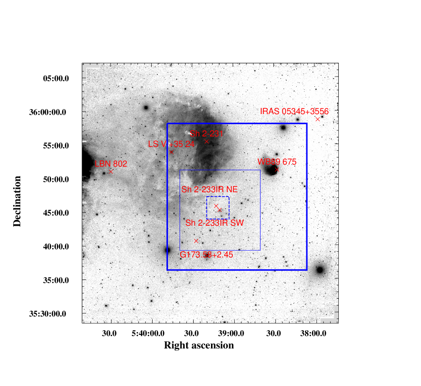
Figure 1: The CFHT $\textrm{H}_{2}$ (bold), CO 3-2 HARP (thin), and CO 2-1 A3 (dashed) fields overlaid on the KPNO $\textrm{H}\alpha$ mosaic with selected objects identified by their SIMBAD names. Sh 2-233IR SW is coincident with IRAS 05358+3543.

2.7 VLA data

VLA archival data from projects AR482, AR513, AS831, and AM697 were re-reduced to perform a deeper search for UCHII regions and aquire more data points on the known UCHII’s SED. Data from AR482 were previously published in Beuther et al. (2007), the other data are unpublished. The data were reduced using the VLA pipeline in AIPS (vlarun). The observations used and sensitivities and beam sizes achieved are listed in Tables 1 and 8. There appeared to be calibration errors in the AR482 observations (the phase calibrator was 2-3 times brighter than in all other observations) and this data were therefore not used in the final analysis, but it produced consistent pointing results.

Table 1: VLA Observation Program Names, Dates, and Times

VLA	Observation	Time	Array	Band	Fluxcal	Phase cal	Phase cal
Observation	Date	on					Percent
Name		Source					Uncertainty
AR482	August 2 2001	2580s	B	X	3c286	0555+398	22
AR513	June 21 2003	7770s	A	X	3c286	0555+398	0.8
AS831	February 26 2005	2640s	B	X	3c286	0555+398	0.7
AS831	August 5 2005	2660s	C	X	3c286	0555+398	0.3
AS831	May 11 2006	2610s	A	X	3c286	0555+398	3.0
AL704	August 7 2007	6423s	A	Q	3c273	0555+398	18
AL704	September 1 2007	6423s	A	Q	3c273	0555+398	13
AM697	November 26 2001	2880s	D	Q	3c286	0555+398	2.2
AM697	November 28 2001	1530s	D	K	3c286	0555+398	2.1
AM697	November 28 2001	1530s	D	U	3c286	0555+398	5.8

3 Results

3.1 Near Infrared Imaging: Outflows and Stars

Eleven distinct outflows have been identified in IRAS 05358 in the images. Outflows are identified from a combination of J=3-2 CO data, shock excited $\textrm{H}_{2}$ emission, and published interferometric maps (Beuther et al. 2002a). Suspected CO outflows were identified by the presence of wings on the CO J=3-2 emission lines that extended beyond the typical velocity range of emission associated with the line core. The single dish data were compared to the interferometric maps of Beuther et al. (2002a). The CFHT $\textrm{H}_{2}$ image was then used to search for shock-excited emission associated with the outflow lobes.

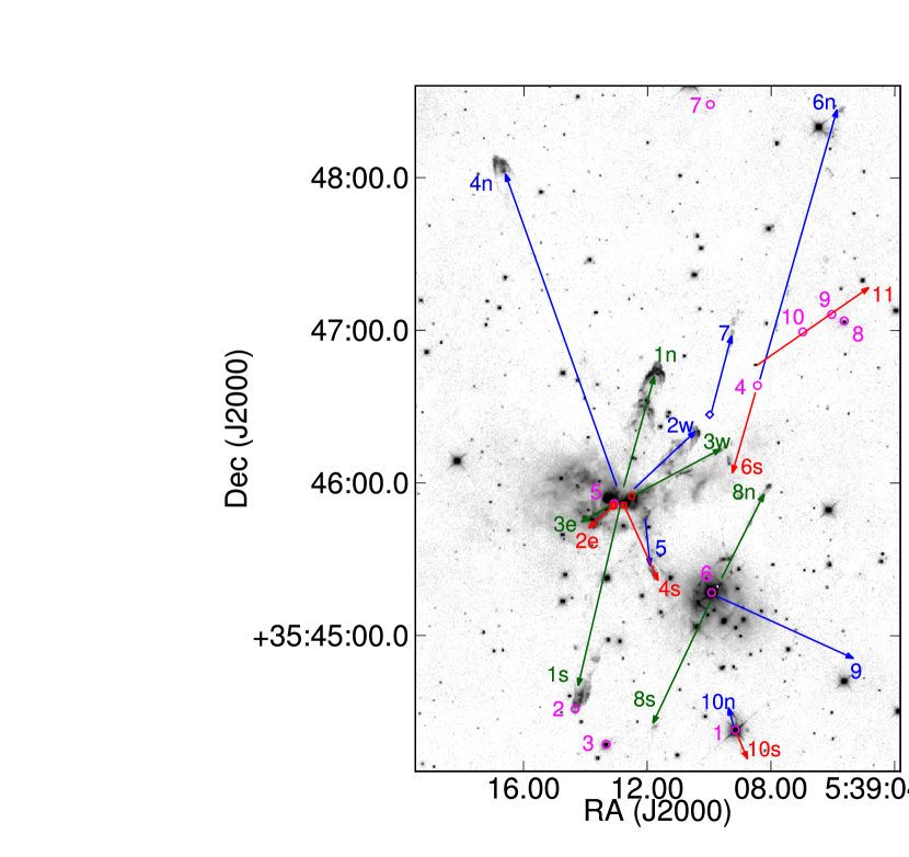
Figure 2: The outflows described in section 4 overlaid on the CFHT $\textrm{H}_{2}$ image. Numbers followed by r and b (red and blue), n and s (north and south), or e and w (east and west) are thought to be counterflows. Red and blue vectors indicate red and blue doppler shifts. Green vectors indicate where the doppler shift is ambiguous or cannot be determined. Magenta circles are Spitzer 24$\mu m$ sources. Red squares are Beuther et al. (2002a) mm sources (from left to right, mm1, mm2, mm3). The blue diamond is a YSO candidate detected only in IRAC bands. The length of the vectors corresponds to the approximate length of the outflows. Source 1 and 6 correspond to Porras et al. (2000) IR 6 and IR 41 respectively, and they are discussed under these names in sections 4. The bows of Outflow 1n and 4n are detected in $\textrm{H}\alpha$ and [S II] emission and are therefore as identified as Herbig-Haro objects HH 993 and 994 respectively.

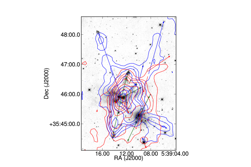
Figure 3: CO contours integrated from $v_{LSR}=$ -13 to -4 km s^-1 (red) and -34 to -21 km s^-1 (blue) at levels of 2,4,6,10,20,30,40,50 K km s^-1 overlaid on the $\textrm{H}_{2}$ image. Specific outflows are labeled in Figure 2 on the same scale.

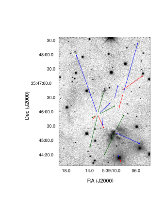
Figure 4: (a) $\textrm{H}_{2}$ image with SO $5_{6}-4_{5}$  peak flux contours at 0.5-1.4 K in intervals of 0.15 K overlaid. With a critical density $\sim 3.5\times 10^{6}$ (Schöier et al. 2005), this transition is a dense gas tracer. (b) The [S II] image with outflow vectors overlaid. Diffuse emission can be seen at the north ends of Outflows 1, 4, and 6 and around the reflection nebula near source IR 41.

Figure 2 shows the $\textrm{H}_{2}$ S(1) 1-0 2.1218 $\mu m$ (a rovibrational transition in the electronic ground state from the $v=1$, $J=3$ to the $v=0$, $J=1$ state) emission in the vicinity of IRAS 05358 with outflows and possible outflow sources labeled. The mm cores from Beuther et al. (2002a) are identified by red squares.

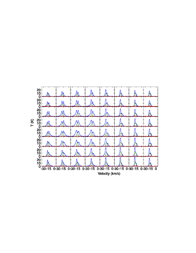
Figure 8: CO spectra of Sh 2-233IR NE in ${}^{12}\textrm{CO}$ (blue), ${}^{13}\textrm{CO}$ (green), and $\textrm{C}^{18}\textrm{O}$ (red). The top-left plot is the pixel centered at J(2000) = 5:39:13.67 +35:46:26.0 and each pixel is 10″ on a side. The region mapped here is shown with a box in Figure 7. Redshifted self-absorption, a possible infall tracer, is evident in the ${}^{12}\textrm{CO}$ spectra in the outer pixels. The inner pixels show self-absorption only at central velocities: this may be an indication that emission from outflows dominates any infall signature, or simply that there is no bulk infall towards Sh 2-233IR NE.

The flow vectors in figure 2 were chosen on the basis of the $\textrm{H}_{2}$ bow shock morphologies and orientations of chains of $\textrm{H}_{2}$ features, association with arcsecond-scale CO features on the Beuther et al. (2002a) Figure 8 CO map, and/or association with lobes of Doppler-shifted CO emission in the CO 3-2 data. The color of the vector indicates the suspected Doppler shift; red and blue correspond to red and blueshifts and green vectors indicate that the Doppler shift is uncertain.

IRAS 05358 outflow 1: The most prominent flow in $\textrm{H}_{2}$ is associated with the bright bow-shocks N1 and N6 (Khanzadyan et al. 2004) located towards PA $\approx$ 345° and 170° respectively from the sub-mm source mms1b (Beuther et al. 2002a). This flow, Beuther et al. (2002a) outflow A, is associated with redshifted and blueshifted CO emission. The northern shock is seen in $\textrm{H}\alpha$ and [S II] emission (figure 4b) and is given a Herbig-Haro designation HH 993.

This flow is indicated by oppositely directed green vectors from the vicinity of smm1, 2, and 3. It is listed as “Jet 1” in Qiu et al. (2008). Kumar et al. (2002) identified the knot immediately behind the bow shock as a Mach disk. In the Beuther et al. (2002a) interferometric maps, the north flow contains redshifted features and the south flow contains primarily blueshifted features. There are also blueshifted CO features to the west of the $\textrm{H}_{2}$ knots that are probably part of a different flow that is not seen in $\textrm{H}_{2}$ emission.

The velocity of the flow as measured from $\textrm{H}_{2}$ emssion is blueshifted as much as 80 km s^-1(LSR), but one component is blueshifted only 14 km s^-1 (see table 3), which is consistent with the cloud velocity. A redshifted SiO lobe is present in the south counterflow. The presence of $\textrm{H}\alpha$, [S II], and [O III] emission in the north shock and corresponding nondetections in the south shock suggest that there is substantially greater extinction towards the south knot. While the velocities in three of the four apertures picked along the TripleSpec slit are blueshifted, there are also knots with velocities consistent with the cloud velocity. Porras et al. (2000) measure the velocity of the counterflow to be -17.3 km s^-1, which is consistent with the cloud velocity. Outflow 1 is propagating very nearly in the plane of the sky.

A line connecting the two bow shocks in Outflow 1 goes directly through Beuther et al. (2007) source mm2a despite the clear association in the Beuther et al. (2002a) interferometric CO map (their Figure 8) with mm1a. The currently available data do not clarify which is the source of the outflow: while the bent CO outflow appears to trace Outflow 1 back to mm1a, there are additional parallel CO outflows towards the confused central region that could originate from either mm1a or mm2a.

A Spitzer 4.5 $\mu m$ and 24 $\mu m$ source is barely detected in $\textrm{H}_{2}$ 2.5′ to the north of Outflow 1. It is only apparent when the $\textrm{H}_{2}$ image is smoothed and would have been dismissed as noise except for the association with a probably 4.5 $\mu m$ extended source. It is labeled 24$\mu m$ source 7 in figure 2. It appears to be slightly resolved at 4.5$\mu m$, and is therefore likely shocked emission. The object may be a protostellar source with an associated outflow, but its proximity to the projected path of Outflow 1 suggests that it may be an older outflow knot.

IRAS 05358 Outflow 2: The second brightest $\textrm{H}_{2}$ features trace a bipolar flow emerging from the immediate vicinity of the sub-mm cluster at PA $\approx$ 135° (red lobe) and 315° (blue lobe). It is listed as “Jet 2” in Figure 6 of Qiu et al. (2008). The counterflow probably overlaps in the line of sight with the counterflow from Outflow 3. It is shorter on the counterflow side either because it has already penetrated the cloud and is no longer impacting any ambient gas or, more likely, it has slowly drilled its way out of the molecular cloud and has not been able to propagate as quickly as the northwest flow. The $\textrm{H}_{2}$ velocities measured for these knots are $\sim$ 30 km s^-1 blueshifted, or marginally blue of the cloud LSR velocity.

The disk identified in Minier et al. (2000) is approximately perpendicular to the measured angle of Outflow 2 assuming that mm1a is the source of this flow. It is therefore an excellent candidate for the outflow source. A diagram of the mm1a region is shown in figure 13. See Section 3.6 for detailed discussion.

IRAS 05358 outflow 3: The Beuther et al. (2002a) CO and SiO maps reveal a third flow, their outflow B at PA $\approx$ 135°  (red lobe) and 315° (blue lobe). A chain of $\textrm{H}_{2}$ features, Khanzadyan et al. (2004) features N3D and N3E, are probably shocks in this flow. It is listed as “Jet 3” in Qiu et al. (2008). The two chains of $\textrm{H}_{2}$ emission indicate that outflows 2 and 3 are distinct. There also appears to be a counterflow at a shorter distance from the mm cores similar to counterflow 2.

Outflows 2 and 3 may be associated with either redshifted or blueshifted features in the Beuther et al. (2002a) CO and SiO maps. High velocity flows with both parities are present near both the northwest (Beuther et al. (2002a) outflow C) and southeast flow for these jets, but the resolution of the millimeter observations is inadequate to determine which flow is in which direction. Porras et al. (2000) measures $v_{LSR}=-7.5$ km s^-1 for their knot 4A, which corresponds to the blended southeast counterflow of outflows 2 and 3. Their Figure 7 shows a wide line that is probably better represented by two or three blended lines, one consistent with the cloud velocity and the other(s) redshifted. Since Outflow 2 has a measured blueshift and outflow 3 is significantly fainter, the redshifted counterflow emission is probably associated with Outflow 2 and the blueshifted with outflow 3.

IRAS 05358 outflow 4: The JCMT CO data and $\textrm{H}_{2}$ images reveal a large outflow lobe consisting of blue lobes 1 and 4 that form a tongue of blueshifted emission propagating to the northeast at PA $\approx$ 20° (Figure 2) from the cluster of sub-mm cores. A faint chain of $\textrm{H}_{2}$ features runs along the axis of the CO tongue and terminates in a bright $\textrm{H}_{2}$ bow shock located at the northern edge of 2. Several $\textrm{H}_{2}$ knots lie along the expected counterflow direction, but that portion of the field contains multiple outflows and is highly confused. If the counterflow is symmetric with the northeast knot, it extends 2.1 parsecs on the sky.

The bow shock of Outflow 4 is seen in the HII and [S II] images, implying that the extinction is much lower than in the cluster. Two apertures placed along the bow shock reveal that it is blueshifted about 70km s^-1 and may be extincted by as little as $A_{V}\sim.5$. It is designated HH 994.

IRAS 05358 outflow 5: Figure 2 shows a bright chain of $\textrm{H}_{2}$ knots and bow shocks starting about 10″ west of mm3 and propagating south at PA $\approx$ 190°. The SiO maps of Beuther et al. (2002a) show a tongue of blueshifted emission along this chain (their Outflow C). The outflow projects back to H¹³CO⁺ source 3, which is also a weak mm source. A lack of obvious counterflow and the possibility that the knots identified with Outflow 5 could be associated with a number of different crossing flows makes this identification very tentative. Higher spatial resolution observations will be required to determine the association of this outflow.

IRAS 05358 outflow 6: The fourth brightest source in the Spitzer 24$\mu m$ data is located at J(2000) = 05:39:08.5, +35:46:38 (source 5 in the IRAS 05358 section of the Qiu et al. (2008) catalog, referred to in table 3 as Q5) in the middle of the molecular ridge that extends from IRAS 05358 towards the northwest (24$\mu m$ object 4 in figure 2). The star is located at the northwest end of the tongue of 1.2mm emission mapped by (Beuther et al. 2002a) with the MAMBO instrument on the IRAM telescope. This part of the cloud is also seen in silhouette against brighter surrounding emission at 8$\mu m$. At wavelengths below 2$\mu m$, it is fainter than 14-th magnitude and therefore is not listed in the 2MASS catalog, and it is not detected in Yan (2009) down to 19th magnitude in K.

Spitzer data indicates very red colors between 3.6 and 70 $\mu m$, indicating that this object is likely to be a Class I protostar. The SED is fit using the online tool provided by Robitaille et al. (2007). Unfortunately, a wide variety of parameters all achieved equally good fits, so no conclusions are drawn about the stellar mass or other very uncertain parameters. However, the top models all had $A_{V}>20$ and many in the range 30-50, indicating that the line of sight is probably through a thick envelope or disk towards this source.

This source lies at the base of the tongue of blueshifted CO 3-2 emission that extends northwest of IRAS 05358 at PA $\approx$ 345°  and has mass $\sim.5M_{\odot}$. A pair of $\textrm{H}_{2}$ features, Khanzadyan et al. (2004) N12A and N12B are located 30 and 55″ from the suspected YSO, forming a chain along the axis of the blueshifted CO tongue. Khanzadyan et al. (2004) $\textrm{H}_{2}$ knot N3F lies along the flow axis in the redshifted direction.

IRAS 05358 outflow 7: The 20″ long chain of $\textrm{H}_{2}$ knots labeled Khanzadyan et al. (2004) N11 appears to trace part of a jet at PA $\approx$ 345° that propagated parallel to outflow 6 about 20″ to the east. The northwest portion of Outflow C in the Beuther et al. (2002a) SiO map is in approximately the same direction as Outflow 7, and it may represent a redshifted counterflow to the northwest-pointing $\textrm{H}_{2}$ knots. The jet axis passes within a few arc-seconds of a faint and red YSO located at J(2000) = 05 39 10.0, +35 46 27 (blue diamond in figure 2 about 35″ south of the southern end of the $\textrm{H}_{2}$ feature). It may be a 24$\mu m$ source but is lost in the PSF of the bright source at the center of Sh 2-233IR NE. This object is also undetected down to 19th magnitude in the Yan (2009) K-band image.

IRAS 05358 outflow 8: A prominent jet-like $\textrm{H}_{2}$ feature protrudes from the vicinity of Sh 2-233IR SW at PA $\approx$ 335°  and ends in bright knot N9. The feature N5B is is located just outside the ring of $\textrm{H}_{2}$ emission that surrounds the IRAS source at the base of the jet. Towards the southeast, knot N6 is located opposite knot N9 with respect to the southwest cluster. IR 41, the $\textrm{H}\alpha$ emission source, labeled 24$\mu m$ source 6 in figure 2, is probably the source of this outflow.

IRAS 05358 outflow 9: In the Spitzer and K_s images, an infrared reflection nebula opens towards the southwest at PA $\approx$ 245° and points towards a blueshifted CO region. The reflection nebula is also seen in $\textrm{H}\alpha$. It is likely that the CO emission in CO Region 1 (table 2) traces a fossil cavity whose walls provide the scattering surface of the reflection nebula.

IRAS 05358 outflow 10 and IR 6: A bright $\textrm{H}_{2}$ filament protrudes at PA $\approx$ 15° towards the northeast of IR 6 (24$\mu m$ source 1, Qiu et al. (2008) source 8). The star is the third brightest 24$\mu m$ source in the IRAS 05358 region. Since it is visible at visual wavelengths, it is not heavily embedded. Its H$\alpha$ emission and association with an outflow lobe and $\textrm{H}_{2}$ emission suggest that it is a moderate mass Herbig AeBe star associated with the IRAS 05358 complex. The optical spectrum confirms this hypothesis: the star has $\textrm{H}\alpha$ absorption wings on either side of a very bright, asymmetric $\textrm{H}\alpha$ emission profile (see section 3.5).

IR 6 is seen to be the source of Outflow 10. Data for this source is available from $\sim$0.45-24$\mu m$, so the Robitaille et al. (2007) spectral fitter puts strong constraints on the star’s mass and luminosity. The measured mass and luminosity are $M=4.5\pm 0.5$ $M_{\odot}$ and $L=10^{2.3\pm.25}L_{\odot}$, parameters consistent with a B7V ($\pm 1$ spectral class) main sequence star. The range of ages in the models covers $10^{4}-10^{7}$ years but favors stars in the range $10^{5}-10^{6}$ years.

While there is a small clump of redshifted CO emission to the northeast of the object, the $\textrm{H}_{2}$ spectrum shows that the north flow is blueshifted $v_{LSR}\sim-40$km s^-1, and the lack of a visible counterflow suggests that the counterflow may be masked behind an additional extincting medium. The counterflow drawn in figure 2 is not seen in emission but is identified as a probable location for a counterflow because of the confident association of outflow 10n with source IR 6.

IRAS 05358 outflow 11: A chain of $\textrm{H}_{2}$ knots is seen at 2.12$\mu m$ and in the Spitzer 4.5$\mu m$ image. They trace back to either IR 78 or 24$\mu m$ source 4. There is a tongue of redshifted CO 3-2 emission in the same direction as this flow that suggests it may be redshifted.

IR 41: There is an arc-like $\textrm{H}_{2}$ emission feature surrounding the $\textrm{H}\alpha$ emission line star IR 41. This implies that the star is probably a late B-type star with too little Lyman continuum emission to generate a photon-dominated region (PDR) but enough soft UV to excite $\textrm{H}_{2}$. From the measured $\textrm{H}\alpha$ and nondetection of $\textrm{H}\beta$ at the star’s location down to a 5-$\sigma$ limit of 1$\times 10^{-17}$ erg s^-1 $\textrm{cm}^{-2}$Å^-1, a lower limit on the extinction column $A_{V}=15$ is derived. The Robitaille et al. (2007) fitter yields a mass estimate of 7.4$\pm 0.6$$M_{\odot}$and luminosity $L=10^{2.97\pm.16}L_{\odot}$ among the 222 best fits out of a grid of 200,000 model SEDs (fits with $\chi^{2}<5000$). The luminosity is very well constrained, varying only modestly to $L=10^{2.99\pm.15}L_{\odot}$ for the 904 best fits ($\chi^{2}<10000$), while the mass shifts down to $6.5\pm 1.0M_{\odot}$. The mass estimate may be biased by the lower number of high-mass models computed. The star’s mass is most compatible with a main sequence B4V star, though its luminosity is closer to a B5V star. The disk mass is constrained to be $>10^{3}M_{\odot}$. The age is reasonably well constrained to be $T=10^{5.78\pm.12}$ for the best 904 models, but is essentially unconstrained for the best 222. Similarly, the stellar temperature is entirely unconstrained by the fitting process.

The very high values of $\chi^{2}$ would normally be worrisome, but the $\chi^{2}$ statistic only represents statistical error, while the data is dominated by various systematic errors including calibration offsets in the optical/NIR and poor resolution in the far-IR. Therefore, it is not possible to find a perfect model fit, but still possible to put constraints on the physical properties of the source.

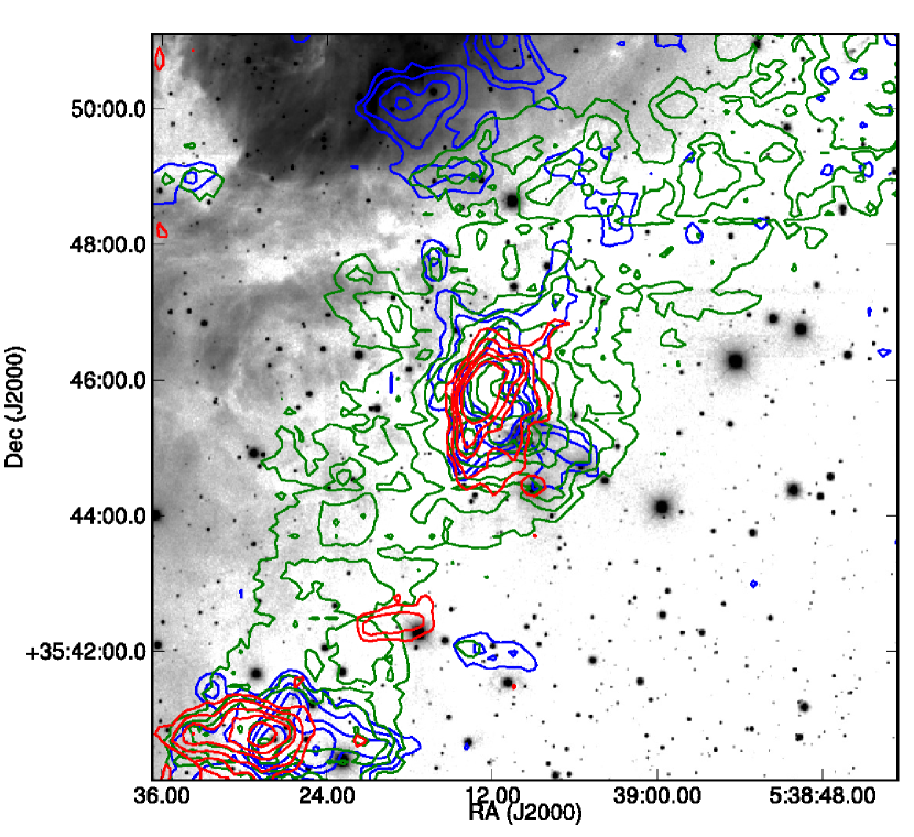
Figure 5: The $\textrm{H}\alpha$ image with CO contours at redshifted, blueshifted, and middle velocities in red, blue, and green respectively. Contours are at 2,4,8,12,20 K km s^-1 for the red and blue, and 20,25,30,40,50,60,70 K km s^-1 for the green. Red is integrated from -12 to -4 km s^-1, Blue from -31 to -21 km s^-1, and green from -21 to -12 km s^-1.

South of IRAS 05358: There is a symmetric flow with one faint $\textrm{H}_{2}$ knot and a bright central source about 4′ south of IRAS 05358. The $\textrm{H}_{2}$ knot is at J(2000) = 05:39:15.63 +35:42:13.2. The flow has a clear red and blue region as identified in figure 6; the red flow extends from -9 to -14 km s^-1 and the blue from -19 to -23 km s^-1 (the outflow is swamped by ambient emission in the intermediate velocity range). The outflow is $\sim 2\arcmin$ long, though the probable source identified is not directly between the two lobes. The ellipses used are labeled in table 2 as Red S and Blue S.

3.2 Imaging results: Optical

Deep [S II] images show that some of the outflows have pierced through the obscuring dust layers or excited extremely bright sulfur emission. Khanzadyan et al. (2004) knot N1 at the end of Outflow 1 is visible [S II] emission The bow of outflow 4 and the northwest end of outflow 6 are detected in [S II]. Only the Outflow 1 and 4 bows are detected in $\textrm{H}\alpha$ emission, indicating that the emission is most likely from shock heating, not external photoionizing radiation. If the shocks were externally irradiated, we would expect the emission to be dominated by the recombination lines. Because they have been detected in the optical, these two flows can be classified as Herbig-Haro objects.

3.3 CO results

IRAS 05358 is located at the center of the CO 3-2 integrated velocity maps (Figure 6). The parent molecular cloud, centered at $v_{LSR}=-17.5$ km s^-1, extends from the southeast towards the northwest with the brightest emission coming from the core associated with Sh 2-233IR SW, while the highest integrated emission is associated with Sh 2-233IR NE. Sh 2-233IR NE has a central velocity of $\sim-16.0$ km s^-1 from the optically thin $\textrm{C}^{18}\textrm{O}$ 2-1 measurements. Material that has been swept up and accelerated by jets and outflows can be seen at velocities $v_{LSR}<-21$ km s^-1and $v_{LSR}>-12$ km s^-1 (Figure 6). The integrated CO 3-2 map peaks at J(2000) = 05:39:12.8 +35:45:55, while the highest observed brightness temperature is at J(2000) = 5:39:09.4 +35:45:12. This offset is discussed in the context of CO isotopologues in section 4.4.2 and in section 5.1.

Regions with line wings relative to the ambient cloud within 5′ of the northeast cluster were assumed to be associated with outflows from the cluster. Further than 5′, it is likely that the high velocity wings are accelerated by neighboring HII regions (see section 5.4). These line wings were integrated over the velocity range -34 to -21 km s^-1 (blue) and -12 to 1 km s^-1 (red) to acquire estimates of the outflowing mass under the assumption that outflowing gas is optically thin. The extracted regions are displayed in Figure 6b and measurements in table 2. The line wings in the central arcminute and central 5 arcminutes were measured for comparison with lower resolution data and to compute a total outflow mass in the central region.

The objects in Table 2 labeled CO Region 1, 2, and 3 have uncertain associations with outflows. CO Region 1 is tentatively associated with outflow 11. CO region 2 may be associated with Outflow 3 but is in a highly confused region and may have many contributors. CO region 3 is probably associated with outflow 10. In contrast, the associations with outflows 4 and 6/7 are more certain because they are further from the central region and less confused. Outflow 1 is seen at high velocities in Beuther et al. (2002a) interferometer maps. Outflow 9 is selected primarily based on CO emission.

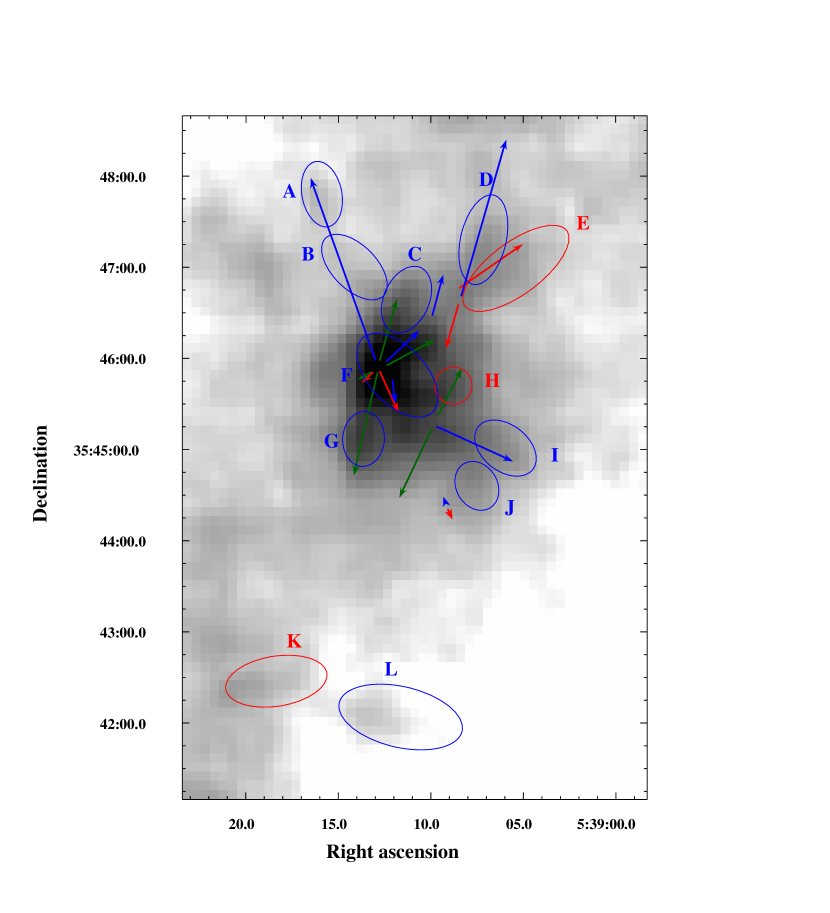
Figure 6: The JCMT HARP CO J=3-2 map integrated over all velocities with significant emission (-34 km s^-1 to -4 km s^-1) shown in gray log scale from 0 to 150 K km s^-1. The elliptical regions over which line wings were integrated are shown with blue and red circles corresponding to blue and red line wings. The measurements are presented in table 2.

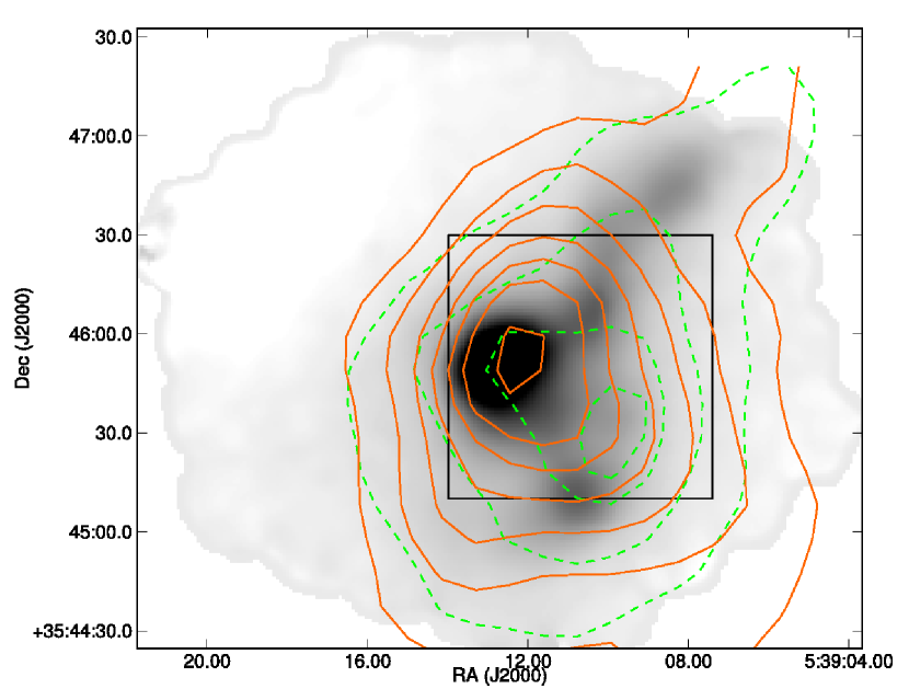
Figure 7: SCUBA 850$\mu m$ image in linear grayscale from -1 to +10 mJy/beam, with a saturated peak of 24 mJy/beam, with ${}^{12}\textrm{CO}$ 2-1 (orange solid, contours at 45,60,85,100,115,130,145 K km s^-1) and ${}^{13}\textrm{CO}$ 2-1 (green dashed, contours at 20,30,40,45 K km s^-1) integrated contours. The box shows the region plotted in Figure 8.

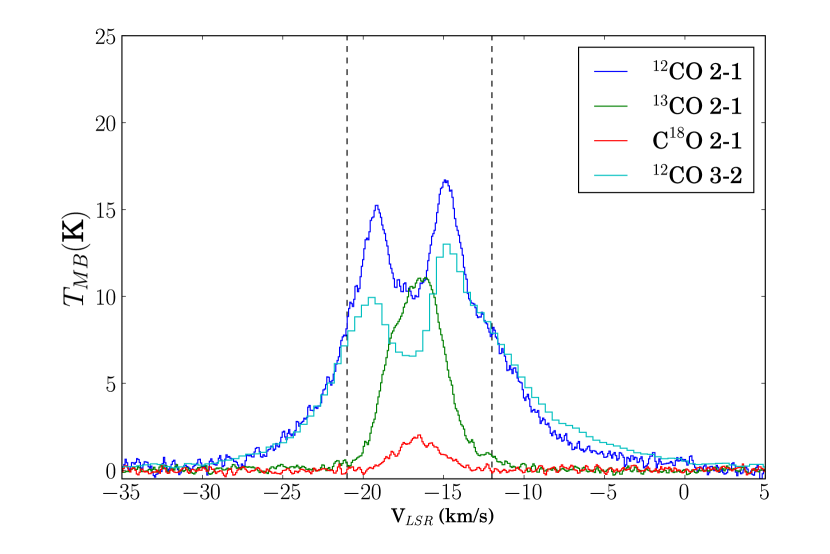
Figure 9: CO spectra of inner 12″ centered on Sh 2-233IR NE for all observed CO lines. The CO 3-2 and 2-1 beams are not matched, but in both cases the area integrated over is 1-2 resolution elements across. The divisions demarcating the red and blue line wings are shown with vertical dashed lines at $v_{LSR}=-21$ and -12 km s^-1.

Table 2: Measured properties of CO flows

Region Name	$\int T_{mb}*$	$M(M_{\odot})$	p ($M_{\odot}$ km s-1)	N ($\textrm{cm}^{-2}$)	E ($10^{42}$ erg)
A. Outflow 4a	4.27	.022	.15	1.4$\times 10^{19}$	11
B. Outflow 4b	4.60	.032	.21	1.5$\times 10^{19}$	13
C. Outflow 1n	14.5	.088	.71	4.8$\times 10^{19}$	66
D. Outflow 6/7	4.45	.045	.30	1.5$\times 10^{19}$	29
E. CO Region 3	1.31	.016	.112	4.3$\times 10^{18}$	8.5
F. Sh 2-233IR NE	41.8	.464	3.72	1.4$\times 10^{20}$	330
F. Sh 2-233IR NE	132.9	1.47	-	4.4$\times 10^{20}$	-
F. Sh 2-233IR NE	30.0	.333	2.03	9.9$\times 10^{19}$	135
G. Outflow1s	14.6	.064	.48	4.8$\times 10^{19}$	40
H. CO Region 2	4.54	.012	.074	1.5$\times 10^{19}$	5
I. Outflow 9	6.33	.039	.39	2.1$\times 10^{19}$	43
J. CO Region 1	3.61	.015	.12	1.2$\times 10^{19}$	11
K. Red S	5.26	.051	.34	1.7$\times 10^{19}$	26
L. Blue S	3.66	.053	.47	1.2$\times 10^{19}$	47
1′ aperture	15.1	.96	7.6	5.0$\times 10^{19}$	670
3′ aperture	2.7	1.6	12	9.0$\times 10^{18}$	1000
5′ aperture	1.7	2.7	20	5.6$\times 10^{18}$	1600
1′ aperture	11.8	0.75	4.7	3.9$\times 10^{19}$	320
3′ aperture	1.9	1.1	6.8	6.2$\times 10^{18}$	460
5′ aperture	0.96	1.5	10	3.2$\times 10^{18}$	640
1′ 12CO 2-1	10.4	.94	7.1	4.9$\times 10^{19}$	590
1′ 12CO 2-1	97.78	8.83	-	4.6$\times 10^{20}$	-
1′ 12CO 2-1	9.17	0.83	5.52	4.3$\times 10^{19}$	430
1′ 13CO 2-1	41.12	211	-	1.1$\times 10^{22}$	-
1′ C18O 2-1	5.31	271	-	1.4$\times 10^{22}$	-

3.4 Near-infrared spectroscopy: Velocities

The slit positions used and apertures extracted from those slits are displayed in Figure 10. Position-velocity diagrams of the 1-0 S(1) line are displayed in Figure 11. Velocity measurements are presented in Table 3.

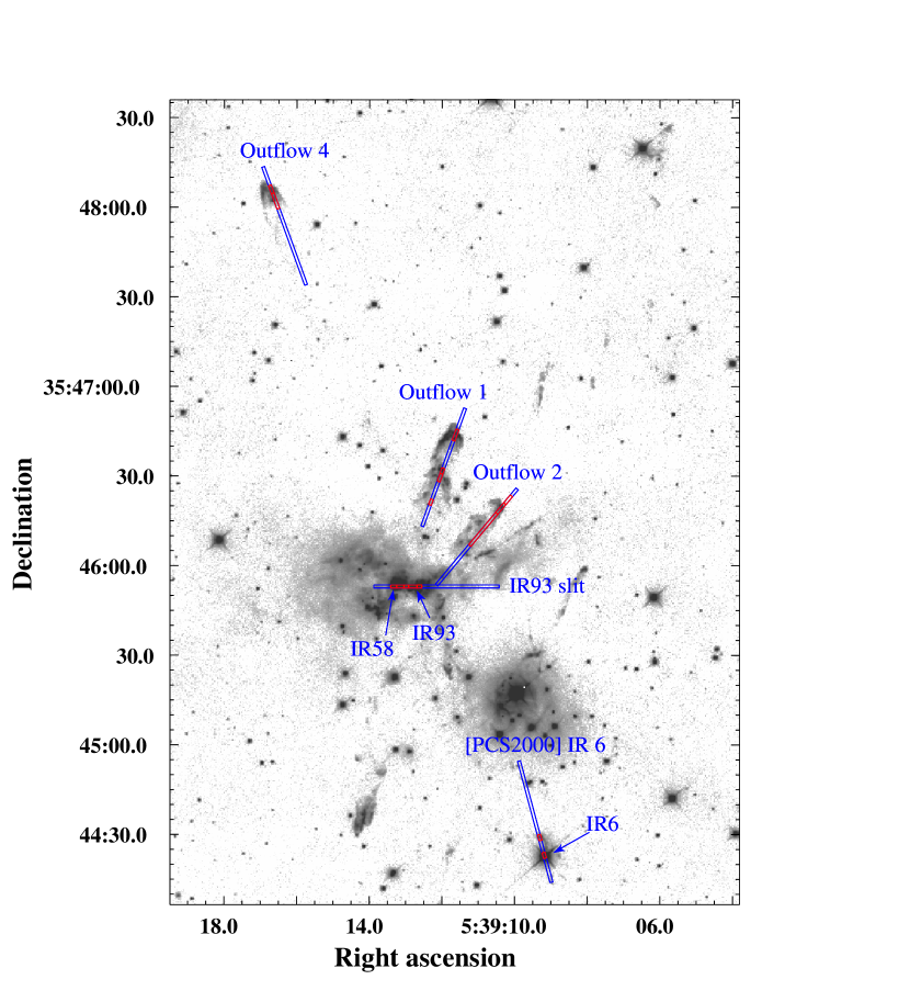
Figure 10: TripleSpec slits (blue) overlaid on the $\textrm{H}_{2}$ image. The red boxes indicate the apertures extracted from those slits to fit and measure $\textrm{H}_{2}$ properties. The apertures are also indicated in the position-velocity diagrams.

The near-IR spectrum of Outflow 1 has the largest signal. All of the K-band $\textrm{H}_{2}$ lines except the 2-1 S(0) 2.3556 $\mu m$ (too weak) and 1-0 S(4) 1.8920 $\mu m$(poor atmospheric transmission) lines were detected (see Table 5). Velocities from gaussian fits to each line are reported. In the central portion of Sh 2-233IR NE, outflowing $\textrm{H}_{2}$ emission at $v_{LSR}\approx-30$ km s^-1 is detected. This material may be associated with a line-of-sight flow, or may originate from the base of the already identified flows 1-3. In source IR 58, Br$\gamma$ and He I 2.05835$\mu m$are detected, indicating that there is an embedded PDR in this source. There is a hint of a second, fainter star adjacent to IR 58. IR 93 is observed to be a double source in the TripleSpec spectrum, but the spectrum is too weak to do any identification. Br$\gamma$ and possibly He I are detected at fainter levels.

Table 5 shows the measured line strengths (when detected) of all $\textrm{H}_{2}$ lines in each aperture. The errors listed are statistical errors that do not include the systematics errors introduced by a failure to correct for narrow atmospheric absorption lines.

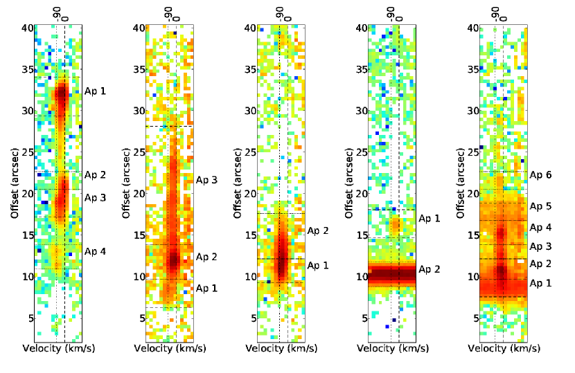
Figure 11: Position-velocity diagrams of the $\textrm{H}_{2}$ 2.1218 $\mu m$ line in Outflows 1,2, 4, IR 6, and IR93/IR58. The velocity range is from -340 to 190 km s^-1.

Table 3: TripleSpec fitted $\textrm{H}_{2}$ outflow velocities

Outflow Number	Aperture Number	vLSR (km s-1)	v${}_{LSR}(\textrm{km~{}s}^{-1})$
1	1	-33.54 (0.15)	-31.85 (0.32)
1	2	-13.60 (0.57)	-13.56 (0.96)
1	3	-40.51 (0.41)	-36.13 (0.81)
1	4	-88.7 (2.8)	-83.7 (7.9)
2	1	-82.6 (7.6)	-81 (21)
2	2	-30.41 (0.57)	-28.9 (1.4)
2	3	-33.89 (0.62)	-35.2 (3.7)
4	1	-73.34 (0.48)	-70.2 (1.1)
4	2	-64.08 (0.61)	-67.8 (2.2)
IR6	1	-39.4 (1.6)	-39.4 (4.2)
IR93	2	-26.07 (0.43)	-26.85 (0.97)
IR93	3	-30.6 (1.5)	-32.0 (2.5)
IR93	4	-29.14 (0.77)	-30.3 (2.1)
IR93	6	-47.7 (7.9)	-71 (37)

Table 4: Measured properties of $\textrm{H}_{2}$ flows

Outflow	Center	PA	Length	Source	Flow	Counterflow	Age	LOS
					Length	Length	(50 km s-1)	Velocity
1	05:39:13.023 +35:45:38.66	-13.3	142.3”	mm2?	58	84.2	1.4e4	-
2	05:39:13.058 +35:45:51.28	-47.0	44.6”	mm1a	44.6	-	6.6e3	Blue
3	05:39:12.48 +35:45:54.9	-62	44”	mm3?	44	-	6.5e3	Red
4	ambiguous	17.8-21.8	141-144”	?	141-144	-	2.1e4	Blue
5	05:39:12 +35:45:51	170	38-48	mm3?	38-48	-	6.5e3	Blue
6	05:39:09.7 +35:45:17	14.5	197	Q5	197	-	2.9e4	Blue
8	05:39:10.002 +35:45:10.87	-154.6	105.5”	IR41?	54.7	52.9	7.9e3	-

Table 5: Measured $\textrm{H}_{2}$ line strengths

	1-0 S(0)	1-0 S(1)	1-0 S(2)	1-0 S(3)	1-0 S(6)	1-0 S(7)	1-0 S(8)	1-0 S(9)	1-0 Q(1)	1-0 Q(2)	1-0 Q(3)	1-0 Q(4)
aperture	2.2233	2.12183	2.03376	1.95756	1.78795	1.74803	1.71466	1.68772	2.40659	2.41344	2.42373	2.43749
outflow1ap1	3.60E-15	9.80E-15	5.50E-15	1.20E-14	4.70E-15	3.10E-15	8.60E-16	1.10E-15	9.20E-15	6.10E-15	1.10E-14	6.90E-15
	( 2.4e-17)	( 3.4e-17)	( 6.8e-17)	( 2e-16)	( 2e-16)	( 2.8e-17)	( 2.8e-17)	( 2.7e-17)	( 1.4e-16)	( 7.4e-17)	( 8.8e-17)	( 7.8e-17)
outflow1ap2	7.10E-16	1.80E-15	9.90E-16	1.80E-15	-	-	-	-	3.00E-15	1.90E-15	3.20E-15	2.00E-15
	( 2.1e-17)	( 2.7e-17)	( 6.8e-17)	( 1.7e-16)	-	-	-	-	( 1.3e-16)	( 4e-17)	( 7.8e-17)	( 3.8e-17)
outflow1ap3	1.60E-15	4.10E-15	2.20E-15	4.70E-15	-	8.30E-16	-	-	5.60E-15	3.70E-15	6.60E-15	4.80E-15
	( 2.4e-17)	( 3.4e-17)	( 6.3e-17)	( 1.8e-16)	-	( 2.8e-17)	-	-	( 1.4e-16)	( 5.9e-17)	( 8.2e-17)	( 5.2e-17)
outflow1ap4	-	9.00E-16	-	-	-	-	-	-	-	-	-	-
	-	( 3e-17)	-	-	-	-	-	-	-	-	-	-
outflow2ap1	-	3.60E-16	-	-	-	-	-	-	-	-	-	-
	-	( 1.5e-17)	-	-	-	-	-	-	-	-	-	-
outflow2ap2	9.40E-16	2.40E-15	1.50E-15	1.80E-15	-	4.00E-16	-	-	3.00E-15	-	3.70E-15	-
	( 1.7e-17)	( 2.2e-17)	( 5.8e-17)	( 1.1e-16)	-	( 2.3e-17)	-	-	( 4.7e-17)	-	( 7.9e-17)	-
outflow2ap3	2.10E-15	1.90E-15	1.80E-15	2.20E-15	-	6.70E-16	-	-	5.70E-15	-	7.30E-15	-
	( 1.7e-17)	( 2.2e-17)	( 5.1e-17)	( 1.3e-16)	-	( 2.9e-17)	-	-	-8.00E-16	-	-8.00E-16	-
outflow4ap1	5.50E-16	2.00E-15	8.50E-16	2.00E-15	-	9.40E-16	1.90E-16	3.40E-16	1.40E-15	-	1.40E-15	-
	( 2e-17)	( 2e-17)	( 5e-17)	( 1.3e-16)	-	( 2.8e-17)	( 1.8e-17)	( 2.3e-17)	-4.00E-16	-	( 6.9e-17)	-
outflow4ap2	5.60E-16	2.00E-15	5.30E-16	2.10E-15	-	5.80E-16	-	1.10E-16	-	-	2.00E-15	-
	( 2e-17)	( 2.2e-17)	( 2.4e-17)	( 1.2e-16)	-	( 2.3e-17)	-	( 1.8e-17)	-	-	-2.00E-16	-
IR6ap1	-	1.10E-15	-	9.30E-16	-	4.30E-16	-	-	-	-	-	-
	-	( 3e-17)	-	( 1.4e-16)	-	( 3.2e-17)	-	-	-	-	-	-
IR93ap1	-	6.60E-15	-	2.70E-15	-	-	-	-	-	-	5.80E-15	-
	-	( 3.5e-17)	-	( 1e-16)	-	-	-	-	-	-	( 7.4e-17)	-
IR93ap2	4.40E-15	6.60E-15	3.90E-15	3.30E-15	-	1.10E-15	-	-	7.60E-15	5.10E-15	6.90E-15	5.50E-15
	( 3.2e-17)	( 3.7e-17)	( 9.2e-17)	( 1.4e-16)	-	( 2.7e-17)	-	-	( 8e-17)	( 5.2e-17)	( 7.4e-17)	( 6.1e-17)
IR93ap3	1.00E-15	1.70E-15	-	9.00E-16	-	-	-	-	2.00E-15	1.70E-15	1.90E-15	-
	( 2.3e-17)	( 3.6e-17)	-	( 1.2e-16)	-	-	-	-	( 8e-17)	( 3.8e-17)	( 8.8e-17)	-
IR93ap4	2.60E-15	3.70E-15	-	-	-	-	-	-	4.30E-15	3.50E-15	4.70E-15	-
	( 3.2e-17)	( 3.6e-17)	-	-	-	-	-	-	( 8.5e-17)	( 5.2e-17)	( 7.4e-17)	-
IR93ap5	-	1.90E-15	-	1.00E-15	-	-	-	-	-	-	-	-
	-	(2.4e-17)	-	(1.00e-16)	-	-	-	-	-	-	-	-
IR93ap6	-	4.10E-16	-	-	-	-	-	-	-	-	-	-
	-	( 3e-17)	-	-	-	-	-	-	-	-	-	-

Note. — Fluxes are in units erg s${}^{-1}\textrm{cm}^{-2}$Å^-1. Errors are listed on the second row for each aperture. Errors of (0) indicate that the line was detected, but that the fluxes should not be trusted because the background was probably oversubtracted.

Table 5: Measured $\textrm{H}_{2}$ line strengths (cont’d)

	2-1 S(1)	2-1 S(3)	3-2 S(3)	3-2 S(4)	4-3 S(5)	[Fe II]	[Fe II]
	2.24772	2.07351	2.2014	2.12797	2.20095	1.6435	1.2567
outflow1ap1	2.00E-15	1.20E-15	6.20E-16	2.60E-16	7.10E-16	4.4e-15	3.5e-15
	( 2.5e-17)	( 3.5e-17)	( 2.2e-17)	( 1.6e-17)	( 1.9e-17)	( 7.9e-17)	( 4e-17)
outflow1ap2	-	-	-	-	-	6.7e-16	3.1e-16
	-	-	-	-	-	( 7.8e-17)	( 3.3e-17)
outflow1ap3	9.90E-16	-	5.70E-16	2.50E-16	6.40E-16	1.3e-15	5.7e-16
	( 2.6e-17)	-	( 0)	( 1.2e-17)	( 0)	( 8.9e-17)	( 4e-17)
outflow1ap4	-	-	-	-	-	-	-
	-	-	-	-	-	-	-
outflow2ap1	-	-	-	-	-	-	-
	-	-	-	-	-	-	-
outflow2ap2	6.40E-16	-	-	-	-	-	-
	( 1.9e-17)	-	-	-	-	-	-
outflow2ap3	-	-	-	-	-	-	-
	-	-	-	-	-	-	-
outflow4ap1	4.30E-16	4.20E-16	-	-	1.60E-16	-	-
	( 1.9e-17)	(0)	-	-	(0)	-	-
outflow4ap2	-	-	-	-	-	-	-
	-	-	-	-	-	-	-
IR6ap1	-	-	-	-	-	-	-
	-	-	-	-	-	-	-
IR93ap1	-	-	-	-	-	-	-
	-	-	-	-	-	-	-
IR93ap2	3.80E-15	-	3.10E-15	-	-	-	-
	( 2.2e-17)	-	(0)	-	-	-	-
IR93ap3	-	-	-	-	-	-	-
	-	-	-	-	-	-	-
IR93ap4	-	-	-	-	-	-	-
	-	-	-	-	-	-	-
IR93ap5	-	-	-	-	-	-	-
	-	-	-	-	-	-	-
IR93ap6	-	-	-	-	-	-	-
	-	-	-	-	-	-	-

Note. — Fluxes are in units erg s${}^{-1}\textrm{cm}^{-2}$Å^-1. Errors are listed on the second row for each aperture. Errors of (0) indicate that the line was detected, but that the fluxes should not be trusted because the background was probably oversubtracted.

3.5 Spectroscopic Results: Optical

IR 6 and IR 41 (objects 1 and 6 in Figure 2) both show $\textrm{H}\alpha$ in emission. IR 41 is close to the reflection nebula in the southeast portion of IRAS 05358 and is probably the reflected star. The reflection nebula’s spectrum is very similar to IR 41’s spectrum at $\textrm{H}\alpha$ in both width and brightness (see Figure 12).

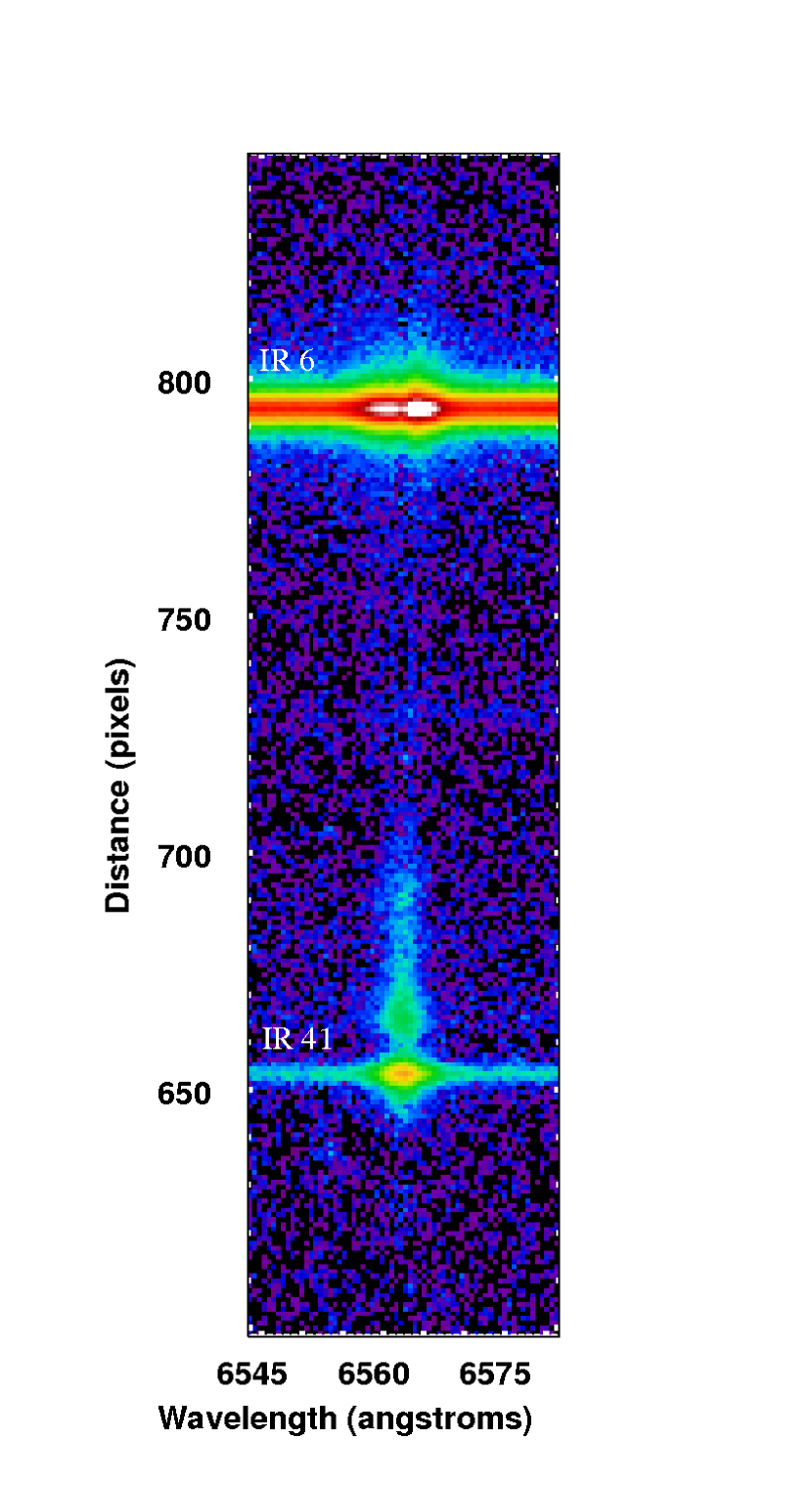
Figure 12: A position-velocity diagram of IR 6 and 41 including the reflection nebula near IR 41 ($\approx 7.4M_{\odot}$). IR 6 shows a two-peaked $\textrm{H}\alpha$ emission profile, but is the less massive ($\approx 4.5M_{\odot}$) of the pair. The separation between the two sources is 55$\farcs$3, and each pixel is 0$\farcs$4.

There are three components in the $\textrm{H}\alpha$ profile of IR 6: a broad absorption feature seen far ($\sim 400\textrm{km~{}s}^{-1}$ from the line center) on the wings and two emission peaks. The peaks are separated by 190 km s^-1 and the blueshifted peak is weaker than the redshifted (Table 6). The H$\beta$ profile shows much deeper absorption and weaker emission but with similar characteristics. The presence of the $\textrm{H}\alpha$ emission makes identification of the stellar type from the $\textrm{H}\alpha$ line profile uncertain. The derived extinction to IR 6 is at least $A_{V}=7$ from an assumed $\textrm{H}\alpha$/$\textrm{H}\beta$ ratio of 2.87 (Osterbrock & Ferland 2006). The $\textrm{H}\beta$ flux was measured from zero to the peaks of the emission profile and therefore probably overestimates the $\textrm{H}\beta$ flux and underestimates the extinction.

Table 6: IR 6 Deblended Profiles

	Blue	Blue	Red	Red	Absorption	Gaussian /	Absorption
	Emission	Wavelength	Emission	Wavelength		Lorentzian FWHM	Wavelength
$\textrm{H}\alpha$	4.4$\times 10^{-14}$	6559.79	1.3$\times 10^{-13}$	6564.23	-2.6$\times 10^{-14}$	1.5 / 0.19	6563.02
$\textrm{H}\beta$	2.4$\times 10^{-14}$	4857.68	1.8$\times 10^{-14}$	4864.28	-4.6$\times 10^{-14}$	0.17 / 16.5	4861.91

Note. — Measurements are made using a Voigt profile fit in the IRAF splot task.

Table 7: Lines observed in the optical spectra

Source	$\textrm{H}\alpha$	$\textrm{H}\beta$	[S II] 6716Å	[S II] 6731Å	[O I] 6300Å	[O I] 6363Å	[O I] 5577Å
Outflow1 ap1	4.3$\times 10^{-16}$	-	5.7$\times 10^{-16}$	6.3$\times 10^{-16}$	5.3$\times 10^{-16}$	1.8$\times 10^{-16}$	-
	6561.49	-	6715.3	6729.6	6299.7	6363.3	-
Outflow1 ap2	4.5$\times 10^{-16}$	-	4.5$\times 10^{-16}$	4.6$\times 10^{-16}$	3.1$\times 10^{-16}$	1.2$\times 10^{-16}$	-
	6561.22	-	6714.9	6729.3	6299.4	6363.2	-
Ambient Medium - slit 1	6.7$\times 10^{-17}$	5.3$\times 10^{-18}$	1.0$\times 10^{-17}$	7.9$\times 10^{-18}$	3.5$\times 10^{-16}$	1.2$\times 10^{-16}$	4.8$\times 10^{-17}$
	6562.87	4861.7	6716.7	6731.2	6300.3	6363.8	5578.0
IR 41 nebula	2.6$\times 10^{-15}$	-	-	-	4.4$\times 10^{-16}$	1.9$\times 10^{-16}$	-
	6562.85	-	-	-	6300.3	6363.9	-
IR 41	6.5$\times 10^{-15}$	-	-	-	1.1$\times 10^{-16}$	7$\times 10^{-17}$	-
	6562.9	-	-	-	6300.0	6363.3	-
IR 6	1.76$\times 10^{-13}$	4.1$\times 10^{-14}$	-	-	-	-
	-	-	-	-	-	-

Note. — Wavelengths listed are in Å and are geocentric. To convert to LSR velocities, subtract 24.35 km s^-1. The ambient medium fluxes represent averages across the slit. Fluxes are in erg s${}^{-1}\textrm{cm}^{-2}$Å^-1.

3.6 Radio Interferometry

A point source was detected in the X, U, K and Q band VLA maps with high significance at the same location as the X-band point source reported in Beuther et al. (2007). Seven-parameter gaussians were fit to each image to measure the beam sizes and positions and flux densities. The measurements are listed in Table 8. The locations of the point source and the shape of the beams from the re-reduced X and Q band images are displayed in figure 13. A Class II 6.7 GHz methanol maser was detected in IRAS 05358 by Menten (1991). It was observed with the European VLBI Network (EVN) by Minier et al. (2000) and seen to consist of a linear string of maser spots that trace a probable disk in addition to maser spots scattered around a line perpendicular to the proposed disk (see Figure 13). The VLA source is more than a VLA beam away from the VLBI CH₃OH maser disk identified by Minier et al. (2000). It is to the southeast in the opposite direction of Outflow 2. Outflow 2 is at position angle -47^∘, while the disk is at PA 25^∘. The 8^∘ difference from being perpendicular is well within the error associated with determining the angle of the outflow in this confused region, so the VLBI disk is a strong candidate for the source of Outflow 2.

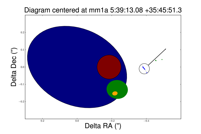
Figure 13: A diagram of the region surrounding mm1a from Beuther et al. (2007). The ellipses are centered at the measured source centers and their sizes represent the beam sizes of the Plateau de Bure interferometer at 1.2mm (blue, Beuther et al. 2007), Gemini MICHELLE at 7.9$\mu m$ (red, Longmore et al. 2006), the VLA at 3.6cm (green), and the VLA at 7mm (orange). The maser disk was measured with the European VLBI Network by Minier et al. (2000), so the size and direction of the disk are very well constrained. The black circle is centered on the pointing center of the VLBI observation and represents the absolute pointing uncertainty. The arrow pointing in the direction of Outflow 2 traces clumps along the outflow back to the mm emission region. The vector is not to scale - Outflow 2 is about 45″ long.

The astrometric uncertainty in VLA measurements are typically $\lesssim 0.1$″. Different epochs of high-resolution X-band and Q-band data confirmed that the pointing accuracy is substantially better than 0.1″ in this case. The VLBI absolute pointing uncertainty is reported to have an upper limit of $\sim 0.03$″ (Minier et al. 2000). The separation between the VLA Q-band center and the VLBI disk center is 0.22″, whereas the separation between the combined X and Q band pointing centers is only 0.027″, which can be viewed as a characteristic uncertainty. This is evidence for at least two distinct massive stars in a binary separated by $\sim$ 400 AU. While the statistical significance of the binary separation is quite high using formal errors, the systematic errors cannot be constrained nearly as well. This object is a candidate binary system but is not yet confirmed.

Table 8: VLA measurements near IRAS 05358 mm1a

Frequency	Beam major /	RA (error)	Peak flux	Map RMS
Observed	minor / PA	Dec (error)	(error)	(mJy/beam)
43.3 GHz	0.022″  / 0.029″ / -10.4 ∘	05:39:13.065425 (0.000015)	1.319 (0.027)	0.179
		35:45:51.14732 (0.00031)
22.5 GHz	1.52″  / 1.28″  / 232 ∘	05:39:13.05521 (0.0029)	1.26 (0.04)	0.091
		35:45:51.378 (0.046)
15.0 GHz	1.58″  / 2.00″  / 0 ∘	05:39:13.062 (0.005)	1.274 (0.065)	0.124
		35:45:51.4 (0.1)
8.4 GHz	0.107″ / 0.122″ / 7.9 ∘	05:39:13.064548 (0.000036)	0.506 (0.003)	0.015
		35:45:51.170356 (0.000613)

4 Analysis

4.1 Near-Infrared Spectroscopic Extinction Measurements

Extinction along a line of sight can be calculated using the 1-0 Q(3) / 1-0 S(1) line ratio.

$$A_{\lambda}=1.09\left[-\textrm{ln}\frac{S_{\nu}(S)/S_{\nu}(Q)}{A_{ul}(S)\lambda_{Q}/A_{ul}(Q)\lambda_{S}}\right]\left[\left(\frac{\lambda_{S}}{\lambda_{Q}}\right)^{-1.8}-1\right]^{-1}$$ (1)

Because they are from the same upper state, their intensity ratio should be set by their Einstein A values times the relative energies of the transitions. However, as shown by Luhman et al. (1998), narrow atmospheric absorption lines in the long wavelength portion of the K band, where the Q branch lines lie, can create a significant bias. Because the lines have not been corrected for atmospheric absorption, the Q branch fluxes should actually be lower limits. Since the 1-0 S(1) transition at 2.1818 microns is affected very little by atmospheric absorption, and the exinction measured is proportional to the Q/S line ratio, the measured extinction should be a lower limit.

The [Fe II] 1.6435 and 1.2567 $\mu m$ lines were detected in Outflow 1, allowing for another direct measurement of the extinction. The measured ratio $FR$ = 1.26$\mu m$/1.64$\mu m$ in Outflow 1 was .8, while the true value is at least 1.24 but may be as high as 1.49 (Smith & Hartigan 2006; Luhman et al. 1998; Giannini et al. 2008). The extinction measured from this ratio ranges from $A_{V}=4.1$ ($FR=1.24$) to 5.8 ($FR=1.49$). The S(1)/Q(3) ratio uncorrected for telluric absorption is .91, which yields an extinction lower limit of $A_{V}=18.7$, is inconsistent with the measurement from [Fe II]. The $\textrm{H}\alpha$ detection and $\textrm{H}\beta$ upper limit give a lower limit on the extinction of $A_{V}=6.6$, which is consistent with both of the other methods to within the calibration uncertainty.

It is possible that the two measurements come from unresolved regions with different levels of extinction, though a factor of at least 3 change over an area $\sim 100AU$ far from the millimeter cores seems unlikely. A strong IR radiation field could plausibly change the line ratio from the expected Einstein A value. The question is not resolved but may be possible to address with near-IR observations of nearby bright HH flows with more careful atmospheric calibration.

4.2 Optical Spectra

4.2.1 Stellar Type

IR 6 is suspected to be the source of the bright $\textrm{H}_{2}$ finger at PA $\approx$ 15°. IR 6 is also a 24$\mu m$ source and was detected by MSX (designation G173.4956+02.4218). We identify this star as a Herbig Ae/Be star.

4.2.2 Density and Extinction Measurements

The spectrum of knot N1 (the bow of Outflow 1) allowed a measurement of electron density in the shocks from the [S II] 6716/6731 line ratio . Densities were determined to be $n=$ 700 $\textrm{cm}^{-3}$  in the forward lump and $n=$500 $\textrm{cm}^{-3}$ in the second lump. $\textrm{H}\alpha$, [N II] 6583, [O I] 6300, and [O III] 6363 were also detected, but no lines were detected in the blue portion of the spectrum presumably because of extinction. The measured velocities from [S II] are faster than the $\textrm{H}_{2}$ velocity measurements at about $v_{LSR}=-68\pm 5$ km s^-1.

There is also an ambient ionized medium that uniformly fills the slit with a [S II]-measured density $n_{e}=120\ \textrm{cm}^{-3}$. Evidently, nearby massive stars are ionizing the low-density ISM located in front of IRAS 05358. This material is moving at velocity $v_{LSR}=-7\pm 5$ km s^-1 and is extincted by $A_{V}=1.5$ as determined from $\textrm{H}\alpha$/H${}_{\beta}=2.87$ assuming the gas is at 10⁴ K.

4.3 UCHII region measurement

A uniform density, ideal HII region will have an intensity curve $I=I_{0}(1-e^{-\tau_{\nu}})$ where

$$\tau=8.235\times 10^{-2}\left(\frac{T_{e}}{K}\right)^{-1.35}\left(\frac{\nu}{\textrm{GHz}}\right)^{-2.1}\left(\frac{\textrm{EM}}{\textrm{pc~{}cm}^{-6}}\right)a(\nu,T)$$ (2)

following Rohlfs & Wilson (2004) equation 9.35, where $a(\nu,T)\approx 1$ is a correction factor. By assuming an excitation temperature $T_{ex}=8500$K, blackbody with a turnover to an optically thin thermal source was fit to the centimeter SED. The turnover frequency from this fit is $\tau=$15.5 GHz, corresponding to an emission measure $EM=7.4\times 10^{8}$ pc cm^-6. This turnover frequency is lower than the $\sim 35$ GHz reported by Beuther et al. (2007). The turnover is clearly visible in the U, K and Q data points in figure 14.

By assuming the X-band emission is optically thick, a source size can be derived.

$$2r=\left[\frac{S_{\nu}}{2k_{B}T_{ex}}\lambda^{2}D^{2}\right]^{1/2}$$ (3)

where D is the distance to the source. Assuming a spherical UCHII region and a distance of 1.8 kpc, the source has radius $r=$30 AU (for comparison, the Q band beam minor axis is $\sim$90 AU, so the region could in principle be resolved by the VLA + Pie Town configuration).

The measured density is $n=(EM/r)^{1/2}=2.2\times 10^{6}$ $\textrm{cm}^{-3}$, with a corresponding emitting mass $M=n\mu m_{H}4/3\pi r^{3}=1.0\times 10^{-6}$ $M_{\odot}$ using $\mu=1.4$. Using Kurtz et al. (1994) equation 1,

$$N_{Lyc}=(8.04\times 10^{46}s^{-1})T_{e}^{-0.85}\left(\frac{r}{pc}\right)^{3}n_{e}^{2}$$ (4)

the number of Lyman continuum photons per second required to maintain ionization is estimated to be $N_{Lyc}=5.9\times 10^{44}$ , a factor of $\sim 4$ lower than measured by Beuther et al. (2007) and closer to a B2 ZAMS star ($\sim 11M_{\odot}$) than B1 using Table 2 of Panagia (1973). If the star has not yet reached the main sequence, it could be significantly more massive (Hosokawa & Omukai 2009), so our stellar mass estimate is a lower limit.

The gravitational binding radius of a 11 $M_{\odot}$ star is $r_{g}=2GM/c_{s}^{2}\approx 190$ AU (the HII region is assumed to be supported entirely by thermal pressure, which provides an upper limit on the binding radius since turbulent pressure can exceed thermal pressure). The UCHII region radius of 30 AU is much smaller, indicating that, under the assumption of spherical symmetry, the HII region is bound.

Leurini et al. (2007) noted that the CH₃CN line profile around this source could be fit with a binary system with separation $<1100$AU and a total mass of 7-22 $M_{\odot}$. This is entirely consistent with our picture of a massive binary system with a 11 $M_{\odot}$ star in a UCHII region and another high mass star with a maser disk.

There are no other sources in the IRAS 05358 region to a 5$\sigma$ limit of 0.075 mJy in the X-band, which provides the strictest upper limit. From equation 3, this corresponds to an optically thick source size of 24 AU. The maser disk has a spatial extent of around 140 AU, so it is quite unlikely that either an undetected UCHII region or the observed UCHII are associated with the maser disk.

Assuming the same turnover point for undetected sources, an upper limit is set on $N_{Lyc}$ for undetected sources:

$$N_{Lyc}=(8.04\times 10^{46}s^{-1})\left(\frac{S_{\nu}}{2k_{B}T_{ex}^{1.85}}\lambda_{cm}^{2}D_{pc}^{2}\right)EM$$ (5)

Our 5$\sigma$ upper limit is $N_{Lyc}=1.38\times 10^{44}$ s^-1, indicating that any stars present must be a later class than B3, or lower than about 8 $M_{\odot}$. For an emission measure as much as 3 times higher, the corresponding stellar mass would be less than 10 $M_{\odot}$. It is likely that no other massive stars have formed in Sh 2-233IR NE.

After independently determining the best-fit UCHII model to the VLA data, we included the PdBI data points from Beuther et al. (2007) and fit a power-law to both data sets. If the emission measure was allowed to vary, the derived parameters were $EM=6.3\times 10^{8}$ and $\beta=0.7$. However, doing this visibly worsened the UCHII region fit without significantly improving the power-law fit, so the fit was repeated holding a fixed emission measure, yielding $\beta=0.8$ (plotted in Figure 14b). This power-law is much shallower than the $\beta=1.6$ measured by Beuther et al. (2007) without access to the 44 GHz data point, and suggests that there is a significant population of large grains in source mm1a. However, we caution that the fits were performed only accounting for statistical errors, not the significant and unknown systematic errors that are likely to be present in mm interferometric data. The PdBI beams are much larger than the VLA beams, so the larger beams could be systematically shifted up by including additional emission, which would reduce $\beta$. Nonetheless, the new VLA data constrains the UCHII emission to contribute no more than 10% of the 3.1mm flux.

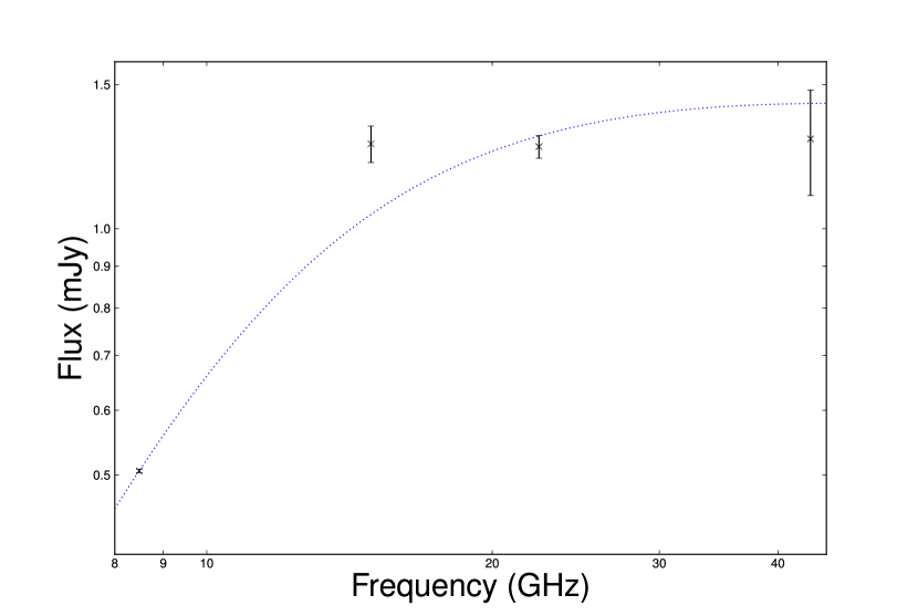
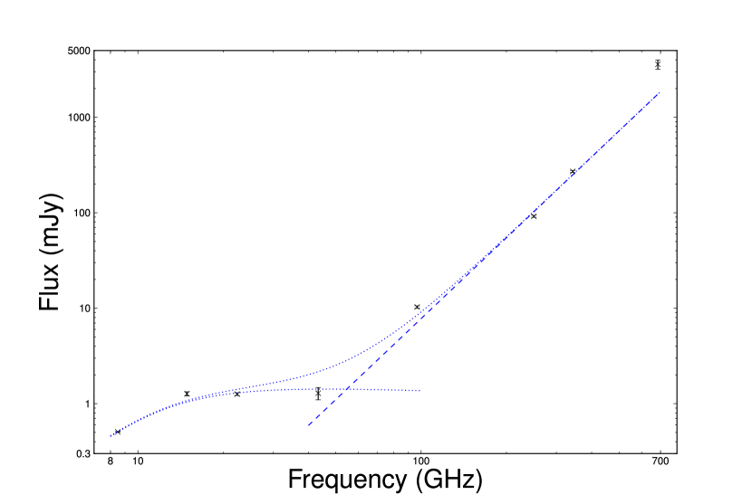
Figure 14: (a) The HII region fit to measured X, K, U, and Q band data. Error bars represent statistical error in the flux measurement. The Q band error is dominated by flux calibration uncertainty (see Table 1). The measured turnover is at 9.5 GHz. (b) A fit to both the VLA data presented in this paper and the (sub)mm points from Beuther et al. (2007). The best fit spectral index for the dust emission is $\alpha=2.8$ ($\beta=0.8$), significantly lower than the $\alpha=3.6$ measured by Beuther et al. (2007) without the 0.7 mm data point.

4.4 Mass, Energy, and Momentum estimates from CO

4.4.1 Equations

The column density for CO J=3-2 is estimated using the equation

$$N_{\textrm{H}_{2}}=\frac{\textrm{H}_{2}}{\textrm{CO}}\frac{8\pi\nu^{3}k_{B}}{3c^{3}hB_{e}A_{ul}}(1-e^{h\nu/k_{B}T_{ex}})^{-1}\frac{1}{\eta_{mb}}\int T_{A}^{*}(v)dv$$ (6)

where $A_{ul}=A_{32}=2.5\times 10^{-6}\textrm{s}^{-1}$ and $A_{21}=6.9\times 10^{-7}$s^-1(Turner et al. 1977), the rotational constant $B_{e}=57.64$, 55.10, and 55.89 GHz for ${}^{12}\textrm{CO}$, ${}^{13}\textrm{CO}$, and $\textrm{C}^{18}\textrm{O}$ respectively, $\eta_{mb}=.68$, and $T_{ex}$ is assumed to be 20K. The partition function is approximated as

$$Z=\sum_{J=1}^{\infty}(2J+1)exp\left(\frac{-J(J+1)hB_{e}}{k_{B}T_{ex}}\right)\approx\int_{0}^{\infty}(2J+1)exp\left(\frac{-J(J+1)hB}{k_{b}T_{ex}}\right)dJ$$ (7)

which is valid when $T_{ex}>>hB_{e}/k_{B}\sim 2.8$K. Equation 6 becomes

$$N_{\textrm{H}_{2}}=(3.27\times 10^{18}\textrm{cm}^{-2})\frac{1}{\eta_{mb}}\int T_{A}^{*}(v)dv$$ (8)

where the integrand is in units K km s^-1. The mass is then

$$M=\mu\ m_{\textrm{H}_{2}}\ A\ N_{\textrm{H}_{2}}=1.42\times 10^{-5}A\frac{1}{\eta_{mb}}\int T_{A}^{*}(v)dv$$ (9)

where A is the area in cm², $\mu=1.4$ is a constant to account for the presence of helium, and again velocity is in km s^-1.

4.4.2 CO J = 2-1 Isotopologue Comparison

Thomas & Fuller (2008) observed C¹⁷O in the J=2-1 and 3-2 transitions each with a single pointing using the JCMT centered at J(2000) = 05:39:10.8 +35:45:16 and measured a column density $N_{\textrm{H}_{2}}=4.03\times 10^{22}$ cm^-2. The peak column density is $1.7\times 10^{22}$$\textrm{cm}^{-2}$ in ${}^{13}\textrm{CO}$ and $2.2\times 10^{22}$ in $\textrm{C}^{18}\textrm{O}$ at J(2000) = 5:39:10.2 +35:45:26, which is reasonably consistent with the C¹⁷O measurement considering abundance uncertainties. The peaks of the integrated spectra for $\textrm{C}^{18}\textrm{O}$ and ${}^{13}\textrm{CO}$ are coincident, but the ${}^{12}\textrm{CO}$ integrated peak is at J(2000) = 5:39:12.6 +35:45:46 (Figure 7, discussed more in section 5.1).

Measurements of the column density, mass, momentum, and energy are performed as in Equation 6. Assuming a ${}^{12}\textrm{CO}$/${}^{13}\textrm{CO}$ ratio of 60 (Lucas & Liszt 1998) and optically thin ${}^{13}\textrm{CO}$, the mean column density across the region is $N_{\textrm{H}_{2}}=4.5\times 10^{21}$ $\textrm{cm}^{-2}$. The resulting total mass of the central $\sim 3$′ is about 320 $M_{\odot}$, which is substantially smaller than the 600 $M_{\odot}$ measured by Beuther et al. (2002a) and Zinchenko et al. (1997), but it is nearly consistent with 870$\mu m$ and NH₃ estimates of 450 and 400 $M_{\odot}$ from Mao & Zeng (2004) and is within the systematic uncertainties of these measurements. Assuming $\textrm{C}^{18}\textrm{O}$ is optically thin and the $\textrm{C}^{18}\textrm{O}$/${}^{13}\textrm{CO}$ ratio is 10, the column density is 5.2$\times 10^{21}$ $\textrm{cm}^{-2}$ and the mass is 360 $M_{\odot}$, which is consistent with the ${}^{13}\textrm{CO}$ measurements, indicating that optical depth effects are probably not responsible for the discrepancy with the dust mass estimate.

4.4.3 CO Mass and Energy Measurements for Specific Outflows

Table 2 lists measurements of mass and momentum in apertures shown in figure 6. Where red and blue masses are listed, there is an outflow in the red and blue along the line of sight. Where only one is listed, an excess to one side of the cloud rest velocity was detected and assumed to be accelerated gas from a protostellar outflow. Blue velocities are integrated from -33 to -21 km s^-1. Red velocities are integrated from -12 km s^-1 to 1 km s^-1. All masses are computed assuming CO is optically thin in the outflow, which leads to a lower bound on the mass; ${}^{13}\textrm{CO}$ 2-1 was measured to have an optical depth of 0.1 in 7 very high velocity outflows in Choi et al. (1993), so if a relative abundance ${}^{12}\textrm{CO}$/${}^{13}\textrm{CO}$= 60 is assumed(Lucas & Liszt 1998), masses increase by a factor of 6.

It is not possible to completely distinguish outflowing matter from the ambient medium. While the outflowing matter is generally at higher velocities, the outflow and ambient line profiles are blended. A uniform selection of high velocities was applied across the region but this may include some matter from the cloud, biasing the mass measurements upward. Outflows in the plane of the sky and low-velocity components of outflows will be blended with the cloud profile, which would lead to underestimates of the outflowing mass. The momentum measurements, however, should be more robust because they are weighted by velocity, and higher velocity material is more certainly outflowing. The momentum measurements are referenced to the central velocity of Sh 2-233IR NE, $v_{LSR}=-16.0$ km s^-1.

5 Discussion

5.1 Outflow Mass and Momentum

Beuther et al. (2002a) reported a total outflowing mass of 20 $M_{\odot}$ in Sh 2-233IR NE. We measure a significantly lower outflow mass of 2 $M_{\odot}$ under the assumption that the gas is optically thin, but this assumption is not valid: a lower limit can be set from the weak ${}^{13}\textrm{CO}$ 2-1 outflow detection (lower limit because not all of the outflowing material is detected) on the outflowing mass of $\sim 4$ $M_{\odot}$. Choi et al. (1993) measure an optical depth of ${}^{13}\textrm{CO}$ 2-1 $\tau\approx 0.1$ in 7 very high velocity outflows. Our ${}^{13}\textrm{CO}$ data suggests that the optical depth is somewhat lower, $\tau\approx 0.07$. The abundance ${}^{12}\textrm{CO}$/${}^{13}\textrm{CO}$= 60 is used (Lucas & Liszt 1998) to derive a total outflowing mass estimate $M\approx 25$ $M_{\odot}$. The total outflowing mass is therefore $\sim 4\%$ of the total cloud mass, though most of the outflowing material is coming from Sh 2-233IR NE, so as much as 13% of the material in Sh 2-233IR NE may be outflowing.

The most prominent outflow in IRAS 05358, Outflow 1, is primarily along the plane of the sky, so the high velocity CO is likely associated with the other outflows that have significant components along the line of sight. As pointed out in Beuther et al. (2002a), the integrated and peak CO are aligned with the main mm core. High-velocity $\textrm{H}_{2}$ near the mm cores and the blueshifted outflows 2 and 4 all suggest that there are many distinct outflows that together are responsible for the high velocity CO gas.

The offset between the integrated ${}^{13}\textrm{CO}$ peak and ${}^{12}\textrm{CO}$ peak in the J=2-1 integrated maps, which corresponds with an offset in the peak of the integrated CO 3-2 map and the peak temperature observed in CO 3-2, suggests that the gas mass is largely associated with Sh 2-233IR SW, but the outflowing gas is primarily associated with Sh 2-233IR NE. The integrated and maximum brightness temperatures in ${}^{13}\textrm{CO}$ and $\textrm{C}^{18}\textrm{O}$ are also centered near Sh 2-233IR SW, which rules out optical depth as the cause of this offset. CO may be depleted in the dense mm cores, which would help account for the lower mass estimate from CO isotopologues relative to dust mass and NH₃. Alternately, the gas temperature in Sh 2-233IR SW may be significantly higher than in Sh 2-233IR NE except in the outflows, which are probably warm. In this case, the outflowing ${}^{12}\textrm{CO}$ enhances the integrated intensity because of its high temperature and reduced effective optical depth, but it does not set the peak brightness because of the low filling-factor of the high-temperature gas.

Because the outflows are seen in $\textrm{H}_{2}$, which requires shock velocities $\sim 30$ km s^-1 to be excited (Bally et al. 2007), and because the association between the high-velocity CO and the plane-of-the-sky $\textrm{H}_{2}$ is unclear, a velocity of 30 km s^-1 is used when estimating the dynamical age. Assuming the outflow is about 0.5 pc long in one direction (e.g. Outflow 1), the dynamical age is 1.6$\times 10^{4}$ years. Outflow 4, which is around 1 pc long, is also seen at a velocity of -70 km s^-1 LSR, or about -50 km s^-1 with respect to the cloud, and therefore has a dynamic age 2$\times 10^{4}$ years, which is consistent.

5.2 Energy Injection / Ejection

Using an assumed outflow lifetime of $5\times 10^{3}$ years for $v=100\ \textrm{km~{}s}^{-1}$ as a lower limit (because the full extent of the flows is not necessarily observed) and $1\times 10^{5}$ as an upper limit (for the CO velocities $\sim 10\ \textrm{km~{}s}^{-1}$ and the longest $\sim 1$ pc flows), mechanical luminosities of the outflows $L=E/t$ are derived. The summed mechanical luminosity of the outflows is compared to the turbulent decay luminosity within a 12″, 1′, and 5′ radius centered on Sh 2-233IR NE in Table 9.

Table 9: Comparison of turbulent decay and outflow injection

Radius (pc)	$t_{turb}$ (yr)	$L_{turb}(L_{\odot})$	$L_{outflows}$ $(L_{\odot})$	Binding Energy (ergs)	Outflow Energy (ergs)	Turbulent Energy (ergs)
0.10	2$\times 10^{4}$	20	0.03-0.6	3.4 $\times 10^{46}$	3.5 $\times 10^{44}$	5.0$\times 10^{46}$
0.52	1$\times 10^{5}$	12	0.6 - 9.4	5.9 $\times 10^{46}$	5.9 $\times 10^{45}$	1.5$\times 10^{47}$
2.62	5$\times 10^{5}$	2.3	1-22	1.2 $\times 10^{46}$	1.4 $\times 10^{46}$	1.5$\times 10^{47}$

The rate of turbulent decay can be estimated from the crossing-time of the region, $L/v$, where $L$ is the length scale and $v$ is the the typical turbulent velocity. On the largest ($\sim$ few pc) scales, the mechanical luminosity from high-velocity outflowing material is approximately capable of balancing turbulent decay and upholding the cloud against collapse. However, at the size scales of the Sh 2-233IR NE clump ($\sim 0.1$ pc), turbulent decay occurs on more than an order of magnitude faster timescales than outflow energy injection. On the smallest scales, outflow energy can be lost from the cluster through collimated outflows, though wide-angle flows and wrapped up magnetic fields will not propagate outside of the core region. Once collimated flows impact the local interstellar medium in a bow shock, their energy and momentum are distributed more isotropically and again contribute to turbulence. The imbalance on a small size scale is consistent with the observed infall signature (Figure 9) in the inner 12″ around Sh 2-233IR NE and the lack of a similar profile elsewhere.

5.3 Comparison to other clumps

The classification scheme laid out in Klein et al. (2005) is used to identify Sh 2-233IR NE as a Protocluster and Sh 2-233IR SW as a Young Cluster. Maury et al. (2009) performed a similar analysis of the Early Protocluster NGC 2264-C. They also found that the outflow mechanical luminosity could provide the majority of the turbulent energy $L_{turb}\sim 1.2L_{\odot}$ within the protocluster in a radius of 0.7 pc with a mass 2300$M_{\odot}$. Williams et al. (2003) performed an outflow study of the OMC 2/3 region with radius 1.2 pc and mass 1100 $M_{\odot}$, which is also an Early Protocluster, and concluded that $L_{turb}\sim L_{flow}\sim 1.3L_{\odot}$. While all three regions have nearly the same turbulent decay luminosities and outflow mechanical luminosities, Sh 2-233IR NE in IRAS 05358 is significantly more compact and lower mass than the Early Clusters, and is the only one of the three that contains signatures of massive star formation.

5.4 Surrounding Regions

About 8′ to the southeast of IRAS 05358 is another embedded star forming region, G173.58+2.45. Interferometric and stellar population studies have been performed by Shepherd & Churchwell (1996) and Shepherd & Watson (2002). The bipolar outflow detected in their interferometric maps is also cleanly resolved in our figure 6. In our wide-field $\textrm{H}_{2}$ maps, there is a complex of outflows similar to that of IRAS 05358, but fainter.

The large HII region Sharpless 231 to the northeast can be seen in the $\textrm{H}\alpha$ image (figure 1). The expanding HII region is pushing against the molecular ridge that includes IRAS 05358 and accelerating the CO gas in the blue direction (e.g. the northern blueshifted clumps in figures 6 and 5). It can be seen from the IRAC 8$\mu m$ data that UV radiation from the HII region reaches to the IRAS 05358 clusters. The expanding HII region’s pressure on the molecular ridge may be responsible for triggering the collapse of IRAS 05358 and G173. The size gradient from S232 ($\sim 30\arcmin$ across) to S231 ($\sim 10\arcmin$) to S233 ($\sim 2-3\arcmin$) is suggestive of an age gradient assuming uniform HII region expansion velocities and a common distance. Investigation of this hypothesis will require detailed stellar population studies in the HII regions with proper regard for eliminating foreground and background sources.

5.5 Massive Star Binary

Our identification of a probable massive star binary with an associated outflow contributes to a very small sample of known maser disks with $\textrm{H}_{2}$ emission perpendicular to the disk. De Buizer (2003) observed 28 methanol maser sources with linear distributions of maser spots in the $\textrm{H}_{2}$ 2.12 $\mu m$ line, and he identified only 2 sources with $\textrm{H}_{2}$ emission perpendicular to the maser lines. None of the outflows identified in his survey were as collimated as Outflow 2, so the methanol disk / outflow combination presented here may be the most convincing association of a massive protostellar disk with a collimated outflow.

The association of a massive star with an UCHII region and a methanol maser disk and the very small size of the UCHII region both suggest that the massive stellar system is very young. Walsh et al. (1998) suggested that the development of a UCHII region leads to the destruction of maser emission regions. Their conclusion is consistent with our interpretation of mm1a as a binary system.

6 Summary & Conclusion

We have presented a multiwavelength study of the IRAS 05358 star forming region. IRAS 05358 contains an embedded cluster of massive stars and is surrounded by outflows. The outflows were linked to probable sources and determined that at least one outflow is probably associated with a massive ($\sim 10M_{\odot}$) star. Added kinematic information and a wide field view of the infrared outflows has been used to develop a more complete picture of the region.

• Sh 2-233IR NE is a Protocluster and Sh 2-233IR SW is a Young Cluster

• Energy injection on the scales of IRAS 05358 can maintain turbulence, but on the small scales of the Sh 2-233IR NE protocluster, is inadequate by $\sim 2$ orders of magnitude. Sh 2-233IR NE is collapsing.

• there are 11 candidate outflows, 7 of which have candidate counterflows, in the IRAS 05358 complex

• there is a probable massive binary with one member of mass 12 $M_{\odot}$ in mm1a, and the other which is the source of Outflow 2

• there are at least two moderate-mass ($\sim$5$M_{\odot}$) young stars in IRAS 05358

We have identified additional middle- and high-mass young stars with outflows, and presented a case for a high-mass binary system within the millimeter core mm1a.

7 Acknowledgements

We would like to thank Vincent Minier for providing us with the positions of the VLBI maser spots and Steve Myers and George Moellenbrock for their assistance with VLA data reduction.

We would also like to thank Cara Battersby, Devin Silvia, Mike Shull, and Jeremy Darling for helpful comments on early drafts.

This work made use of SAOIMAGE DS9 (http://hea-www.harvard.edu/RD/ds9/), IRAF (http://iraf.net/, scipy (http://www.scipy.org), and APLpy (http://aplpy.sourceforge.net/).

References

- Alvarez & Hoare (2005) Alvarez, C. & Hoare, M. G. 2005, A&A, 440, 569
- Bally et al. (2007) Bally, J., Reipurth, B., & Davis, C. J. 2007, in Protostars and Planets V, ed. B. Reipurth, D. Jewitt, & K. Keil, 215–230
- Beuther et al. (2007) Beuther, H., Leurini, S., Schilke, P., Wyrowski, F., Menten, K. M., & Zhang, Q. 2007, A&A, 466, 1065
- Beuther et al. (2002a) Beuther, H., Schilke, P., Gueth, F., McCaughrean, M., Andersen, M., Sridharan, T. K., & Menten, K. M. 2002a, A&A, 387, 931
- Beuther et al. (2002b) Beuther, H., Schilke, P., Sridharan, T. K., Menten, K. M., Walmsley, C. M., & Wyrowski, F. 2002b, A&A, 383, 892
- Casoli et al. (1986) Casoli, F., Combes, F., Dupraz, C., Gerin, M., & Boulanger, F. 1986, A&A, 169, 281
- Choi et al. (1993) Choi, M., Evans, II, N. J., & Jaffe, D. T. 1993, ApJ, 417, 624
- De Buizer (2003) De Buizer, J. M. 2003, MNRAS, 341, 277
- Giannini et al. (2008) Giannini, T., Calzoletti, L., Nisini, B., Davis, C. J., Eislöffel, J., & Smith, M. D. 2008, A&A, 481, 123
- Henning et al. (1992) Henning, T., Cesaroni, R., Walmsley, M., & Pfau, W. 1992, A&AS, 93, 525
- Heyer et al. (1996) Heyer, M. H., Carpenter, J. M., & Ladd, E. F. 1996, ApJ, 463, 630
- Hosokawa & Omukai (2009) Hosokawa, T. & Omukai, K. 2009, ApJ, 691, 823
- Jiang et al. (2001) Jiang, Z., Yao, Y., Yang, J., Ishii, M., Nagata, T., Nakaya, H., & Sato, S. 2001, AJ, 122, 313
- Khanzadyan et al. (2004) Khanzadyan, T., Smith, M. D., Davis, C. J., & Stanke, T. 2004, A&A, 418, 163
- Klein et al. (2005) Klein, R., Posselt, B., Schreyer, K., Forbrich, J., & Henning, T. 2005, ApJS, 161, 361
- Krumholz et al. (2009) Krumholz, M. R., Klein, R. I., McKee, C. F., Offner, S. S. R., & Cunningham, A. J. 2009, Science, 323, 754
- Kumar et al. (2002) Kumar, M. S. N., Bachiller, R., & Davis, C. J. 2002, ApJ, 576, 313
- Kurtz et al. (1994) Kurtz, S., Churchwell, E., & Wood, D. O. S. 1994, ApJS, 91, 659
- Lada & Lada (2003) Lada, C. J. & Lada, E. A. 2003, ARA&A, 41, 57
- Leurini et al. (2007) Leurini, S., Beuther, H., Schilke, P., Wyrowski, F., Zhang, Q., & Menten, K. M. 2007, A&A, 475, 925
- Longmore et al. (2006) Longmore, S. N., Burton, M. G., Minier, V., & Walsh, A. J. 2006, MNRAS, 369, 1196
- Lucas & Liszt (1998) Lucas, R. & Liszt, H. 1998, A&A, 337, 246
- Luhman et al. (1998) Luhman, K. L., Engelbracht, C. W., & Luhman, M. L. 1998, ApJ, 499, 799
- Mao & Zeng (2004) Mao, R.-Q. & Zeng, Q. 2004, Chinese Journal of Astronomy and Astrophysics, 4, 440
- Maury et al. (2009) Maury, A. J., André, P., & Li, Z.-Y. 2009, A&A, 499, 175
- Menten (1991) Menten, K. M. 1991, ApJ, 380, L75
- Minier et al. (2000) Minier, V., Booth, R. S., & Conway, J. E. 2000, A&A, 362, 1093
- Osterbrock & Ferland (2006) Osterbrock, D. E. & Ferland, G. J. 2006, Astrophysics of gaseous nebulae and active galactic nuclei, ed. D. E. Osterbrock & G. J. Ferland
- Panagia (1973) Panagia, N. 1973, AJ, 78, 929
- Parker et al. (1991) Parker, N. D., Padman, R., & Scott, P. F. 1991, MNRAS, 252, 442
- Porras et al. (2000) Porras, A., Cruz-González, I., & Salas, L. 2000, A&A, 361, 660
- Qiu et al. (2008) Qiu, K. et al. 2008, ApJ, 685, 1005
- Reipurth & Bally (2001) Reipurth, B. & Bally, J. 2001, ARA&A, 39, 403
- Robitaille et al. (2007) Robitaille, T. P., Whitney, B. A., Indebetouw, R., & Wood, K. 2007, ApJS, 169, 328
- Rohlfs & Wilson (2004) Rohlfs, K. & Wilson, T. L. 2004, Tools of radio astronomy (Tools of radio astronomy, 4th rev. and enl. ed., by K. Rohlfs and T.L. Wilson. Berlin: Springer, 2004)
- Scalise et al. (1989) Scalise, Jr., E., Rodriguez, L. F., & Mendoza-Torres, E. 1989, A&A, 221, 105
- Schöier et al. (2005) Schöier, F. L., van der Tak, F. F. S., van Dishoeck, E. F., & Black, J. H. 2005, A&A, 432, 369
- Shepherd & Churchwell (1996) Shepherd, D. S. & Churchwell, E. 1996, ApJ, 457, 267
- Shepherd & Watson (2002) Shepherd, D. S. & Watson, A. M. 2002, ApJ, 566, 966
- Smith & Hartigan (2006) Smith, N. & Hartigan, P. 2006, ApJ, 638, 1045
- Thomas & Fuller (2008) Thomas, H. S. & Fuller, G. A. 2008, A&A, 479, 751
- Turner et al. (1977) Turner, J., Kirby-Docken, K., & Dalgarno, A. 1977, ApJS, 35, 281
- Valdes & Swaters (2007) Valdes, F. G. & Swaters, R. A. 2007, in Astronomical Society of the Pacific Conference Series, Vol. 376, Astronomical Data Analysis Software and Systems XVI, ed. R. A. Shaw, F. Hill, & D. J. Bell, 273–+
- Walsh et al. (1998) Walsh, A. J., Burton, M. G., Hyland, A. R., & Robinson, G. 1998, MNRAS, 301, 640
- Wang et al. (2003) Wang, H., Yang, J., Wang, M., & Yan, J. 2003, AJ, 125, 842
- Williams et al. (2003) Williams, J. P., Plambeck, R. L., & Heyer, M. H. 2003, ApJ, 591, 1025
- Williams et al. (2004) Williams, S. J., Fuller, G. A., & Sridharan, T. K. 2004, A&A, 417, 115
- Wouterloot et al. (1993) Wouterloot, J. G. A., Brand, J., & Fiegle, K. 1993, A&AS, 98, 589
- Yan (2009) Yan, C. 2009, ApJ
- Zinchenko et al. (1997) Zinchenko, I., Henning, T., & Schreyer, K. 1997, A&AS, 124, 385