Anderson Impurity in Helical Metal

Abstract

We use a trial wavefunction to study the spin-1/2 Kondo effect of a helical metal on the surface of a 3-dimensional topological insulator. While the impurity spin is quenched by conduction electrons, the spin-spin correlation of the conduction electron and impurity is strongly anisotropic in both spin and spatial spaces. As a result of strong spin-orbit coupling, the out-of-plane component of the impurity spin is found to be fully screened by the orbital angular momentum of the conduction electrons.

On the surface of a 3-dimensional (3D) topological insulator, massless helical Dirac fermions emerge.Fu1 Specific materials of 3D topological insulators have recently been studied and observed.Hsieh ; Xia ; zhang-nphys ; Chen Interesting properties of these helical Dirac fermions have become a focus of recent studies.Fu2 ; Qi ; Law ; Tanaka In a helical metal, spins are coupled to momenta, so that magnetic properties are expected to be highly non-trivial. Theoretical study on this aspect, however, has so far been limited to the effect of a classical magnetic impurity.magneticimp

The low temperature property of a quantum spin-1/2 magnetic impurity or an Anderson impurity in a conventional metalAnderson has been an interesting and important problem for decades in condensed matter physics. The problem has been studied by using the renormalization groupWilson , the Bethe ansatzWiegmann ; Andrei , the $1/N$-expansionColeman ; Gunnarsson , and the conformal field theoryAffleck . The phenomenon is a well known Kondo effect, in which the impurity spin is completely screened by the conduction electrons. Because of the coupling between spins and momenta, the Kondo effect in a helical metal will be interesting to be examined. In this paper, we use a variational method to address this problem. We show that the correlation of the impurity spin and the conduction electron spin density is strongly anisotropic in both spatial and spin spaces, in contrast to the isotropic screening in a conventional metal. While the impurity spin is quenched at low temperatures, similar to the usual Kondo problem, the correlation between the impurity spin and the spin of the conduction electrons in the helical metal is significantly reduced. The reduction of the spin-spin correlation in the direction perpendicular to the surface can be shown explicitly to be compensated by the screening of the orbital angular momentum of the conduction electrons. The possible experimental consequences will be briefly discussed.

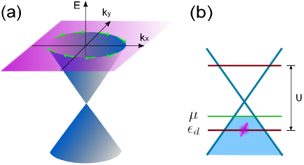
Figure 1: (color online). (a) Schematic energy-momentum dispersion in a helical metal. Electron spin (green arrow) is perpendicular to momentum. (b) Energy diagram of a helical metal with a singly occupied Anderson impurity state at energy $\epsilon_{d}$ in the absence of their coupling $H_{mix}$ in Eq. (Anderson Impurity in Helical Metal). $\mu$ is the chemical potential.

We consider a spin-1/2 magnetic impurity in a helical metal in a 2D $x$-$y$ plane, described by the Hamiltonian,

$$H =H_{c}+H_{mix}+H_{d}$$

$$H_{c} =\sum_{\mathbf{k}}c^{{\dagger}}_{\mathbf{k}}[\hbar v_{F}(\boldsymbol{\sigma}\times\mathbf{k})\cdot\hat{z}-\mu]c_{\mathbf{k}}$$

$$H_{mix} =\sum_{\mathbf{k}}V_{\mathbf{k}}c^{{\dagger}}_{\mathbf{k}}d+h.c.$$

$$H_{d} =(\epsilon_{d}-\mu)(n_{d\uparrow}+n_{d\downarrow})+Un_{d\uparrow}n_{d\downarrow}.$$

In the above equations, $c_{\mathbf{k}}$ and $d$ are annihilation operators of the conduction electron with momentum $\mathbf{k}$ and of the $d$-electron at impurity site in the spinor representation, respectively. $\boldsymbol{\sigma}$ are the Pauli matrices, $\mu$ is the chemical potential, and $n_{d\sigma}=d^{\dagger}_{\sigma}d_{\sigma}$. $H_{c}$ describes a helical metal, and $H_{d}$ is a local impurity Hamiltonian with $\epsilon_{d}$ the impurity energy level and $U$ the Coulomb repulsion energy of the two $d$-electrons on the same impurity site. $H_{mix}$ is a hybridization term between the helical metal and the impurity state.

To start with, let us discuss the simple case $H_{mix}=0$ first. In this limit, the helical metal and the impurity state are decoupled. The single electron eigen-energy and its corresponding eigenstate of the helical metal $H_{c}$ are given by

$$\epsilon_{\mathbf{k}\pm} = \pm\hbar v_{F}|\mathbf{k}|-\mu$$

$$\gamma_{\mathbf{k}\pm} = \frac{1}{\sqrt{2}}(e^{\frac{i}{2}\theta_{\mathbf{k}}}c_{\mathbf{k}\uparrow}\pm ie^{-\frac{i}{2}\theta_{\mathbf{k}}}c_{\mathbf{k}\downarrow})$$ (2)

with $\theta_{\mathbf{k}}$ the angle of the momentum $\mathbf{k}$ with respect to the $x$-axis that $\tan{\theta_{\mathbf{k}}}=k_{y}/k_{x}$ and ”$\pm$” refer to upper and lower bands, respectively. For each single particle state, its spin lies in the plane and is perpendicular to the direction of its momentum. Note that such a spin-momentum relation has recently been reported in a spin- and angle-resolved photoemission spectroscopy (spin-ARPES) experiment sARPES . The ground state of $H_{c}$ is then given by

$$|\Psi_{0}\rangle=\prod_{\{\mathbf{k}\pm\}\in\Omega}\gamma^{{\dagger}}_{\mathbf{k}\pm}|0\rangle,$$

where the product runs over all the states within the Fermi sea $\Omega$. As for the impurity part, we shall consider an interesting case, where $\epsilon_{d}<\mu<\epsilon_{d}+U$, so that the impurity site is singly occupied and has a local moment. The total energy of the system $H_{0}=H_{c}+H_{d}$ is then

$$E_{0}=\epsilon_{d}-\mu+\sum_{\{\mathbf{k}s\}}\epsilon_{\mathbf{k}s},$$

where $s=\pm$ is the band index and hereafter the sum of $\{\mathbf{k}s\}$ is always over the Fermi sea. In Fig. 1, we illustrate the electron dispersion and the spin of the Dirac fermion and the ground state of a helical metal, in the absence of the hybridization with the impurity state.

To study the ground state of $H$ in the presence of $H_{mix}$, we will use a trial wavefunction approach. Such a trial wavefunction method was used to study the ground state of the Anderson impurity problem in the conventional metalVarma ; Gunnarsson or in an antiferromagnetVarma2 . For simplicity, we consider here the large U limit, and exclude the double d-electron occupation at the impurity site. We expect the qualitative physics should apply to the case of finite but large U. The trial wavefunction for the ground state is,

$$|\Psi\rangle=(a_{0}+\sum_{\{\mathbf{k}s\}}a_{\mathbf{k}s}d^{{\dagger}}_{\mathbf{k}s}\gamma_{\mathbf{k}s})|\Psi_{0}\rangle$$ (3)

where $d_{\mathbf{k}\pm}=\frac{1}{\sqrt{2}}(e^{\frac{i}{2}\theta_{\mathbf{k}}}d_{\uparrow}\pm ie^{-\frac{i}{2}\theta_{\mathbf{k}}}d_{\downarrow})$, and $a_{0}$ and $a_{\mathbf{k}s}$ are variational parameters . They are to be determined by optimizing the ground state energy. Note that by construction, the impurity state is either singly occupied or non-occupied.

The energy of $H$ in the variational state $|\Psi\rangle$ is given by

$$E=\frac{\sum_{\{\mathbf{k}s\}}(E_{0}-\epsilon_{\mathbf{k}s})a_{\mathbf{k}s}^{2}+2V_{\mathbf{k}}a_{0}a_{\mathbf{k}s}+\epsilon_{\mathbf{k}s}a_{0}^{2}}{a_{0}^{2}+\sum_{\{\mathbf{k}s\}}a_{\mathbf{k}s}^{2}}$$ (4)

The variational method leads to the equations below,

$$(E-\sum_{\{\mathbf{k}s\}}\epsilon_{\mathbf{k}s})a_{0} = \sum_{\{\mathbf{k}s\}}V_{\mathbf{k}}a_{\mathbf{k}s}$$ (5)

$$(E-E_{0}+\epsilon_{\mathbf{k}s})a_{\mathbf{k}s} = V_{\mathbf{k}}a_{0}$$ (6)

which may determine the binding energy $\Delta_{b}\equiv E_{0}-E$ due to the hybridization,

$$\epsilon_{d}-\mu-\Delta_{b}=\sum_{\{\mathbf{k}s\}}\frac{|V_{\mathbf{k}}|^{2}}{\epsilon_{\mathbf{k}s}-\Delta_{b}}.$$ (7)

If $\Delta_{b}>0$, the hybridized state is stable against the decoupled state. To proceed further, we introduce an energy cutoff $\Lambda$ for the helical metallic state in our analysis, and consider $V_{\mathbf{k}}=V\Theta(\Lambda-\hbar v_{F}|\mathbf{k}|)$, where $\Theta(x)$ is a step function, which is 1 for $x>0$ and 0 for $x<0$. The low energy physics is expected to be insensitive to the cutoff $\Lambda$. A natural energy cutoff for the helical metallic state in the topological insulator is the half of the bulk gap.Chen Eq.(7) enables us to determine the ground state energy $E$ or the binding energy $\Delta_{b}$ and the ground state wavefunction. The results are that the hybridization always leads to a binding $\Delta_{b}>0$, and a magnetic screening of the conduction electrons to the impurity spin at any $\mu\neq 0$. At the Dirac point $\mu=0$, the binding and screening only occur at the dimensionless hybridization strength $\alpha=\frac{2\pi V^{2}}{\hbar^{2}v_{F}^{2}}$ above a critical value. We will come back to this point later.

We shall first examine the magnetic properties of the system, which are most interesting. The central quantity we will examine is the correlation function of the impurity spin $\mathbf{S_{d}}=\frac{1}{2}d^{\dagger}\boldsymbol{\sigma}d$ at the impurity site (set to be at the origin $\mathbf{r}=0$) and the conduction electron spin density $\mathbf{S_{c}}=\frac{1}{2}c^{\dagger}(\mathbf{r})\boldsymbol{\sigma}c(\mathbf{r})$ in the ground state, namely

$$J_{uv}(\mathbf{r})\equiv\langle S_{c}^{u}(\mathbf{r})S_{d}^{v}(0)\rangle,$$ (8)

where $\langle Q\rangle$ is the ground state average of $Q$, and $u,v=x,y,z$ are the spin indices. If $u$ and $v$ are both on the $x-y$ plane, we then have, by the rotational symmetry, $J_{uv}(\mathbf{r})=J_{u^{\prime}v^{\prime}}(\mathbf{r^{\prime}})$, if $u^{\prime}=R_{z}(\beta)u$, $v^{\prime}=R_{z}(\beta)v$, and $\mathbf{r^{\prime}}=R_{z}(\beta)\mathbf{r}$, with $R_{z}(\beta)$ a rotational operator of angle $\beta$ along the z-axis. $J_{\mu,\nu}(\mathbf{r})$ can be calculated by using the trial wave-function in Eq. (3). Note that the variational parameter $a_{\mathbf{k}\pm}$ is independent of $\theta_{\mathbf{k}}$ since it can be expressed as $Va_{0}/(\pm\hbar v_{F}|\mathbf{k}|-\mu-\Delta_{b})$ according to the Eq. (6). In terms of $a_{\mathbf{k}\pm}$, the diagonal components are found to be

$$J_{zz}(\mathbf{r}) = -\frac{1}{8}|\mathcal{B}(\mathbf{r})|^{2}+\frac{1}{8}|\mathcal{A}(\mathbf{r})|^{2}$$

$$J_{xx}(\mathbf{r}) = -\frac{1}{8}|\mathcal{B}(\mathbf{r})|^{2}-\frac{1}{8}Re(\mathcal{A}^{2}(\mathbf{r}))$$

$$J_{yy}(\mathbf{r}) = -\frac{1}{8}|\mathcal{B}(\mathbf{r})|^{2}+\frac{1}{8}Re(\mathcal{A}^{2}(\mathbf{r}))$$

where $\mathcal{A}(\mathbf{r})=\sum_{\{\mathbf{k}s\}}se^{i(\mathbf{k}\cdot\mathbf{r}+\theta_{\mathbf{k}})}a_{\mathbf{k}s}$ and $\mathcal{B}(\mathbf{r})=\sum_{\{\mathbf{k}s\}}e^{i\mathbf{k}\cdot\mathbf{r}}a_{\mathbf{k}s}$. $J_{zz}(\mathbf{r})=J_{zz}(r)$ is rotational symmetric around the impurity site, while $J_{xx}(\mathbf{r})$ and $J_{yy}(\mathbf{r})$ are highly anisotropic in space. In Fig. 2, we show $J_{zz}(r)$ and $J_{yy}(x,0)$. Note that $J_{xx}(x,0)=J_{zz}(x,0)$ and their signs oscillate in space. A negative (positive) value means anti-parallel (parallel) correlation between the impurity spin and the conduction electron spin density. Due to the absence of the spin $SU(2)$ symmetry, the off-diagonal components are not zero in general and they are

$$J_{xy}(\mathbf{r}) = J_{yx}(\mathbf{r})=-\frac{1}{8}Im(\mathcal{A}(\mathbf{r})^{2}),$$

$$J_{xz}(\mathbf{r}) = -J_{zx}(\mathbf{r})=\frac{1}{4}Im(\mathcal{B}(\mathbf{r})\mathcal{A}(\mathbf{r})),$$

$$J_{yz}(\mathbf{r}) = -J_{zy}(\mathbf{r})=-\frac{1}{4}Re(\mathcal{B}(\mathbf{r})\mathcal{A}(\mathbf{r})).$$

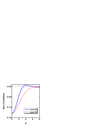
Figure 2: (color online). Spatial Spin-spin correlation functions $J_{yy}(x,0)$ and $J_{zz}(x,0)$ ($J_{xx}(x,0)=J_{zz}(x,0)$) in Eq. (8) as functions of $x$, for a set of parameters $\Delta_{b}=0.005\Lambda$ and $\mu=-0.01\Lambda$. The length unit is $\hbar v_{F}/\Lambda$. Different parameters show qualitatively similar feature as long as $\Delta_{b}>0$.

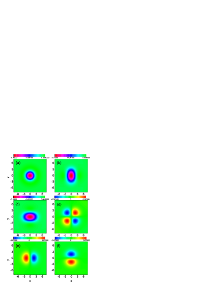
Figure 3: (color online). Spatial spin-spin correlation functions plotted in x-y plane. (a)$J_{zz}(x,y)$; (b)$J_{xx}(x,y)$; (c)$J_{yy}(x,y)$; (d)$J_{xy}(x,y)$ or $J_{yx}(x,y)$; (e)$J_{xz}(x,y)$ or $-J_{zx}(x,y)$); (f)$J_{yz}(x,y)$ or $-J_{zy}(x,y)$. The parameters are the same as those in Fig. 2.

The spatial distributions of the spin correlations in 2D are plotted in Fig. 3. As we can see, the magnitude of $J_{yy}(\mathbf{r})$ is larger at the space point $\mathbf{r}$ near the $x$-axis than near the $y$-axis, and the magnitude of $J_{xx}(\mathbf{r})$ is larger at the space point $\mathbf{r}$ near the $y$-axis than near the $x$-axis.

The anisotropic spin correlation function implies that the Kondo screening to a magnetic impurity in a helical metal has more complex texture. In the strong spin-orbit coupled system, the screening to the impuriy spin may be contributed from both the spin and orbital angular momentum of the conduction electrons. In what follows, we will show that in comparison with the Kondo effect in a conventional metal, the spin-spin screening is largly reduced, and the z-component of the impurity spin is fully screened by the orbital angular momentum. Let us first examine the correlation between the total spin of the conduction electron, $\mathbf{S_{c}}=\int\mathbf{S_{c}(\mathbf{r})}d^{2}\mathbf{r}$ and the impurity spin. We define

$$I_{u}=\langle S_{c}^{u}S_{d}^{u}\rangle/\sum_{\{\mathbf{k}s\}}a_{\mathbf{k}s}^{2},$$

with $u=x,y,z$, where the denominator is the occupation number of the d-electron. $I=\sum_{u}I_{u}$ is a measure of spin-spin screening strength. $I=0$ if the conduction electron and impurity state are decoupled. $I=-3/4$ for a spin-1/2 magnetic impurity in a conventional metal, corresponding to a spin singlet of two spin-1/2. In the present helical metal, when the Fermi level is at or below the Dirac point, we find $I_{x}=I_{y}=-\frac{1}{8}$ and $I_{z}=0$, therefore $I=-\frac{1}{4}$, which is one third of the value of $-3/4$ in the usual Kondo problem. Note that although $J_{zz}$ is non-zero locally, its overall contribution to the spin-spin screening is zero. The spin-spin screening comes from the in-plane spin components. Since $I$ is independent of any parameters including the energy cutoff (the only requirement is $\mu<0$), we expect that this is a general property of the helical metal. When the Fermi level is above the Dirac point, there is a deviation from the above result. For instant, with the parameters $\mu=0.01\Lambda$ and $\Delta_{b}=0.005\Lambda$ the deviation is about sixty percents of $-1/4$. At $\mu>0$, the upper Dirac cone is partially filled. The electron state in the upper Dirac cone has spin orientation opposite to the corresponding state in the lower Dirac cone, which provides a stronger screening than induced by the lower band only. We remark that the difference between $\mu<0$ and $\mu>0$ is due to the particle-hole asymmetry in our model parameter with U large. If $U+2(\epsilon_{d}-\mu)=0$, we have particle-hole symmetry, and we expect correponding symmetries for $\mu<0$ and $\mu>0$.

The conduction electron spin is not a good quantum number in a helical metal. To better understand the Kondo screening in the helical metal, we shall consider contribution from the orbital angular momentum. Because of the two dimensionality, only z-component of the orbital angular momentum can be considered here. The system is invariant with respect to a simultaneous rotation of both spin and space along the z-axis at the origin of the impurity site. Therefore, the z-component of the total angular momentum $J^{z}=L^{z}+S_{c}^{z}+S_{d}^{z}$ commutes with the Hamiltonian H and is a good quantum number, where $L^{z}$ is the total orbital angular moment of the conduction electrons. Since the ground state preserves the time reversal symmetry, we have $J^{z}|\Psi\rangle=0$. Because of this and $\langle S_{c}^{z}S_{d}^{z}\rangle=0$ discussed above, we have

$$\frac{\langle L^{z}S_{d}^{z}\rangle}{\sum_{\{\mathbf{k}s\}}a_{\mathbf{k}s}^{2}}=\frac{\langle J^{z}S_{d}^{z}-S_{c}^{z}S_{d}^{z}-(S_{d}^{z})^{2}\rangle}{\sum_{\{\mathbf{k}s\}}a_{\mathbf{k}s}^{2}}=-\frac{1}{4}.$$ (9)

Therefore, although spin-spin screening in the z-direction in the present Kondo problem vanishes, the orbital angular momentum $L^{z}$ replaces the role of the conduction electron spin $S_{c}^{z}$ to screen the impurity spin.

The spatial anisotropic correlations may be detected in spin resolved scanning tunneling spectroscope (STM) experiments. The magnetic susceptibility is finite in this variational theory. In the light of the unconventional spin correlations, exactly how the susceptibility behaves has to be answered by more elaborate treatments such as quantum Monte Carlo and numerical renormalization group. This issue is left for further investigations.

We now discuss the binding energy $\Delta_{b}$ of the system. From Eq. (7), we obtain

$$\epsilon_{d}-\mu-\Delta_{b}+\alpha(\Lambda-|\mu|)$$ (10)

$$= \alpha(\mu+\Delta_{b})\ln{\frac{4(\Lambda+\mu+\Delta_{b})\Delta_{b}}{(\mu+|\mu|+2\Delta_{b})^{2}}}$$

In the limit of small $\alpha$, and $\alpha\Lambda<\mu-\epsilon_{d}$, we have

$$\Delta_{b} \approx\Lambda\exp{\left[-\frac{\mu-\epsilon_{d}-\alpha\Lambda}{\alpha|\mu|}\right]} ,\mu<0$$

$$\Delta_{b} \approx\frac{\mu^{2}}{\Lambda}\exp{\left[-\frac{\mu-\epsilon_{d}-\alpha\Lambda}{\alpha|\mu|}\right]} ,\mu>0.$$ (11)

If the Fermi level is at the Dirac point, $\mu=0$, $\Delta_{b}$ has a positive value solution only if $\alpha>\alpha_{c}=|\epsilon_{d}|/\Lambda$. In other words, for a given hybridization strength $\alpha$, there is a critical value of the impurity $d$-level, below which there is no magnetic screening. This is due to the vanishing density of states at the Dirac point. This result is similar to the impurity problem in graphene. Sengupta ; Zhuang . The binding energy as functions of the chemical potential $\mu$ and the hybridization $\alpha$ are plotted in Fig. 4.

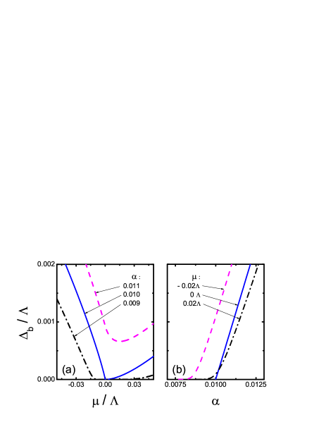
Figure 4: (color online). Binding energy $\Delta_{b}$ as functions of the chemical potential $\mu$ and the hybridization strength $\alpha$. $\Lambda$ is an energy cutoff.

$\Delta_{b}$ is asymmetric about the point $\mu=0$. The solid curves in Fig. 4 are for $\alpha=\alpha_{c}$ and $\mu=0$ respectively. At $\alpha>\alpha_{c}$, the hybridized state is always stable. At $\alpha<\alpha_{c}$, the binding energy is strongly reduced around the Dirac point and vanishes at $\mu=0$. As $\alpha\rightarrow\alpha_{c}+0^{+}$, $\Delta_{b}\approx|\alpha-\alpha_{c}|\Lambda$. This behavior is consistent with the result by using large-degeneracy method.Withoff

In summary, we have examined a spin-1/2 Anderson impurity in a 2D helical metal. The momentum-dependent spin orientation in the helical metal shows interesting magnetic properties. We have used a trial wavefunction method to study the system at the large Coulomb U limit. While the impurity spin is quenched by the conduction electrons, we find strong spin- and spatial-anisotropies in the correlations between the impurity spin and the conduction electron spin density. Because of the strong spin-orbit coupling, the orbital angular momentum also contributes significantly to the screening of the impurity spin. In particular, the out-of-plane component of the impurity spin is found to be fully screened by the orbital angular momentum of the conduction electrons. After our paper was submitted, there was a report on the experimental realization of the magnetic doping on the surface of the 3D topological insulator Bi2Se3 Cha , and a e-print by Zitko, who studied the essentially the same model as ours and mapped it onto a conventional Ander- son pseudogap impurity model.Zitko He showed that the impurity spin is fully screened. Our trial wave-function method reported here is consistent with his result.

Finally we comment on the similarity and difference of the helical metal with the graphene. In terms of the eigen-energy problem, a helical metal is often considered to be a quarter of a graphene, where the pseudospin plays the similar role with the spin in helical metal. The graphene has a two-fold spin degeneracy and two-fold degeneracy associated with the two sublattices. Our results for the binding energy are similar to the graphene. However, because of the difference between the spin in the helical metal and the pseudospin in graphene, the magnetic properties of the two are different. If we consider only one of the two Dirac cones is coupled to the spin-1/2 impurity, the graphene behaves like a conventional metal.

We acknowledge useful discussions with Yi Zhou and Naoto Nagaosa, and acknowledge partial support from HKSAR and RGC. QHW was supported by NSFC (under the Grant Nos.10974086 and 10734120) and the Ministry of Science and Technology of China (under the Grant No. 2006CB921802).

References

- (1) L. Fu, C. L. Kane and E. J. Mele, Phys. Rev. Lett. 98, 106803 (2007).
- (2) D. Hsieh, et al, Nature 452,970-974 (2008).
- (3) Y. Xia, et al. Nature Physics 5 398 (2009).
- (4) H. J. Zhang et al, Nature Physics 5, 438 (2009).
- (5) Y. L. Chen, et al Science 325, 178-181 (2009).
- (6) L. Fu and C. L. Kane, Phys. Rev. Lett. 100, 096407 (2008).
- (7) X. L. Qi et al, Science 323, 1184 (2009).
- (8) K. T. Law, P. A. Lee and T. K. Ng, Phys. Rev. Lett. 103, 237001 (2009).
- (9) Y. Tanaka, T. Yokoyama and N. Nagaosa, Phys. Rev. Lett. 103, 107002 (2009).
- (10) Q. Liu, C. X. Liu, C. Xu, X. L. Qi and S. C. Zhang , Phys. Rev. Lett. 102, 156603 (2009).
- (11) P. W. Anderson, Phys. Rev. 124, 41 (1961).
- (12) H. R. Krishna-murthy, J. W. Wilkins, K. G. Wilson, Phys. Rev. B 21 1003 (1980).
- (13) A. M. Tsvelick and P. B. Wiegmann. Z. Phys. B 54, 201 (1984).
- (14) N. Andrei and C. Destri, Phys. Rev. Lett. 52, 364 (1984).
- (15) F. C. Zhang and T. K . Lee, Phys. Rev. B 28, 33 (1983); F. C. Zhang and T. K. Lee, Phys. Rev. B30 1556 (1984); P. Coleman, Phys. Rev. B29, 3035 (1984); N. Read and D. M. Newns, J. Phys. C, 16, 3273 (1983); Y. Kuramoto, Z. Phys. 53 37 (1983).
- (16) O.Gunnarsson and K. Schnhammer, Phys. Rev. Lett. 50, 604 (1983).
- (17) I. Affleck, Nucl. Phys. B 336, 517 (1990).
- (18) D.Hsieh et al, Nature 460, 1101-1105 (2009)
- (19) C. M. Varma and Y. Yafet, Phys. Rev. B13, 2950 (1976).
- (20) V. Aji, C. M. Varma, and I Vekhter, Phys. Rev. B77, 224426 (2008).
- (21) K. Sengupta and G. Baskaran, Phys. Rev. B77, 045417 (2008).
- (22) H. B. Zhuang et al, EPL 86, 58004 (2009).
- (23) D. Withoff and E. Fradkin, Phys. Rev. Lett. 64, 1835 (1990).
- (24) J.J. Cha, et al, arXiv:1001.5239 (2010)
- (25) R. Zitko, arXiv:1003.5581 (2010)