A fresh look at the seismic spectrum of HD49933:
analysis of 180 days of CoRoT photometry

Abstract

Context. Solar-like oscillations have now been observed in several stars, thanks to ground-based spectroscopic observations and space-borne photometry. CoRoT, which has been in orbit since December 2006, has observed the star HD49933 twice. The oscillation spectrum of this star has proven difficult to interpret.

Aims. Thanks to a new timeseries provided by CoRoT, we aim to provide a robust description of the oscillations in HD49933, i.e., to identify the degrees of the observed modes, and to measure mode frequencies, widths, amplitudes and the average rotational splitting.

Methods. Several methods were used to model the Fourier spectrum: Maximum Likelihood Estimators and Bayesian analysis using Markov Chain Monte-Carlo techniques.

Results. The different methods yield consistent result, and allow us to make a robust identification of the modes and to extract precise mode parameters. Only the rotational splitting remains difficult to estimate precisely, but is clearly relatively large (several $\mu$Hz in size).

1 Introduction

Stars are now the objects of seismic studies after decades of similar studies for the Sun, thanks to the advent of space-borne photometric observations (e.g., MOST, CoRoT and Kepler) and extremely precise ground-based spectroscopic observations (for a complete review, see for e.g. Aerts et al., 2008). This applies in particular to stars presenting solar-like p modes (acoustic oscillations stochastically excited by convection), with CoRoT observations of such stars showing clearly individual peaks in the Fourier spectra (e.g. Michel et al., 2008). Among these stars, HD49933 has already been the target of asteroseismic campaigns. It was first observed spectroscopically from the ground for 10 nights (Mosser et al., 2005). In 2007, a first photometric time series of 60 days was collected by CoRoT, followed by a new long run of 137 days in 2008. HD49933 is a F5 main sequence star with an apparent visual magnitude $m_{V}=5.77$. It is hotter than the Sun ($T_{\rm eff}$=6780 K or $T_{\rm eff}$=6500 K, Bruntt et al., 2008; Bruntt, 2009; Ryabchikova et al., 2009) with an estimated mass of $\sim 1.2M_{\odot}$ (Mosser et al., 2005) and an estimated radius of $1.34\pm 0.06\,R_{\odot}$ (Thévenin et al., 2006). The surface rotation ($v\sin i$) was determined to be around 10 km s^-1 (Mosser et al., 2005; Solano et al., 2005). The surface rotation period has also been measured at $\sim$ 3.4 days, using the 60-day CoRoT timeseries (Appourchaux et al., 2008; Deheuvels et al., 2008), from the signatures of photospheric transiting active regions (e.g., spots) which give rise to a clear peak in the very low-frequency part of the Fourier spectrum.

The seismic interpretation of HD49933 has proven to be very difficult. Mosser et al. (2005) could not isolate individual p modes in the Fourier spectrum of observed line-of-sight velocities but were able to find a regular pattern in the spectrum, which is the signature of the large frequency separation between modes of same degree $l$ (but increasing radial order $n$). The first CoRoT time-series was analysed by Appourchaux et al. (2008), and these data clearly show individual p-mode peaks in the Fourier spectrum. However, the peaks show large widths, making the interpretation less than straightforward: a given peak could be interpreted as being a closely spaced pair of $l$=0 and $l$=2 modes, or a single (but rotationally split) $l$=1 mode. Based on the modeling of the spectrum using a Maximum Likelihood Estimator fitting method, Appourchaux et al. (2008) chose one of these two possible interpretations (hereafter called model A) based on the highest likelihood of each model. This first time-series was the object of other studies. Appourchaux et al. (2009) put into perspective the results of Appourchaux et al. (2008), showing that the likelihood ratio test does not give the probability of the hypothesis given the data, but only the significance of the data given the hypothesis. Benomar et al. (2009), who applied a Bayesian analysis to the same time series, could not definitely favour one interpretation (model A) over the alternate (model B), based on the whole probability distribution of each model. Gruberbauer et al. (2009), using a Bayesian approach too, also consider the identification ambiguous. Gaulme et al. (2009) used a simpler Bayesian approach (Maximum A Posteriori, or MAP, approach). The most probable model they found corresponds to the same identification as Appourchaux et al. (2008). More recently, Mosser & Appourchaux (2009) proposed an empirical method to determine the identification of the modes. Its application considers the model B as the more likely when using the two datasets used here.

It should be noted that the case of HD49933 is quite different from the solar case: solar modes are very narrow in comparison. Their widths (1 $\mu$Hz for the modes with the highest amplitudes) are much smaller than the small-frequency separations between $l$=0 modes of order $n$ and the neighbouring $l$=2 modes of order $n$-1 (being typically around 10 $\mu$Hz for the Sun). Moreover, the star inclination angle, if small, tends to attenuate the visibility of mode components with azimutal order $m\neq 0$, making the mode identification even more difficult.

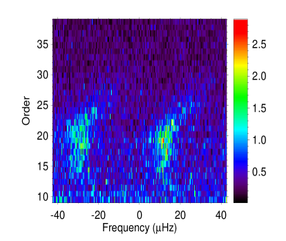
Figure 5: Echelle diagram computed for a large separation of 85 $\mu$Hz for the mean power spectrum. The diagram is smoother to 0.8 $\mu$Hz. The identification of the ridges is far from evident. The most probable model correspond to $l=1$ for the left ridge and $l=0$ for the right ridge (same convention as in Fig. 3)

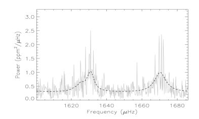
Figure 8: Detail of the spectrum (solid grey line), and of the fitted model (dashed line) with a pair $l=0/2$ on the left and an $l=1$ on ther right.

Here, we use the new long-run CoRoT observations of HD49933, together with the original shorter run timeseries (Fig. 7), in order to properly describe the acoustic oscillations of the star clearly visible in the Fourier spectrum (Fig. 1, Fig. 5 and Fig. 8).

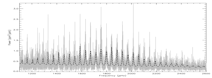
Figure 1: Mean power spectrum using 3 time series of 60 days (solid grey line), and the fitted model (dashed line).

2 Methodology

The time series used here were extracted in the same way as in Appourchaux et al. (2008). The gaps in the series represent slightly less than 10% and were filled by linear interpolation. In order to provide a robust seismic interpretation of the CoRoT timeseries for HD49933, several analyses were performed, using different methods (Maximum Likelihood Estimators, or MLE; and various Bayesian analyses); or the same method applied in an independent manner. These methods were already used in the same way to analyze the initial run of 60 days (Appourchaux et al., 2008; Benomar et al., 2009). The “fitters” of Appourchaux et al. (2008) and some additional fitters sought to find a best-fitting model spectrum. The model has several contributions. There is a contribution from the background, which includes signatures of convection and possibly phenomena with longer time scales (e.g. those related to the stellar activity) and contributions from the individual p modes. Each mode is described by a set of parameters: a central frequency, a width and a height. A single height and width was fitted to each $l=0$/2 pair and the closest $l=1$ mode (in frequency). The relative heights of the $l$=0, 1 and 2 modes took fixed values, which were assumed to be independent of frequency. A single rotational frequency splitting parameter was fitted to all non-radial modes. The stellar inclination, which governs the relative heights of the different $m$ components for a given ($n$,$l$) mode, was also fitted as a single, global parameter. The observed spectrum used by the different fitters was an averaged spectrum (frequency resolution 0.19 $\mu$Hz) made from three timeseries of the same duration, which came from the two CoRoT runs: the first 60-day run, IRa01, and two 60-day long timeseries from the longer second run, LRa01 (data available at idoc-CoRoT.ias.u-psud.fr). The different fitters analysed this spectrum independently, and we then compared the results.

3 Results

The availability of the new longer CoRoT timeseries makes the mode (degree $l$) identification significantly less ambiguous than it was before. The p-mode peaks are still observed to be very wide (several $\mu$Hz), and the typical signal-to-noise ratio (SNR) (defined as the ratio of the height of a mode to the level of the background around the mode) is similar to that for the first, shorter CoRoT run. However, the additional information provided by the longer second run is sufficient to allow the modes to be tagged with far greater confidence than was hitherto possible. There was a very good agreement between the results of the fitters, with model B (which has an $l$=1 mode at 1755 $\mu$Hz; see Table 1 for details) favoured strongly over Model A. As part of the analysis for this paper, we performed a Bayesian analysis (using the method described by Benomar, 2008; Benomar et al., 2009) to compare model A with model B, and this now favours model B at a confidence level higher than 99 %. It is important to add that this confidence level does depend to some extent upon the hypothesis used for the modeling (e.g. on the a priori constraints applied to the model parameters). Here, the 99 % level was estimated for a model with fixed mode height ratios (see Section 2 above). When the fixed height ratio constraint was relaxed so that individual heights were fitted to modes of different $l$, we found that the confidence level for model B dropped no lower than 95 %. (It is worth adding that the average fitted height ratio agrees, to within errors, with the solar-like value we adopted as the fixed height ratio.)

We also established, using the Bayesian approach, that models that include $l=2$ modes are strongly favoured over those which do not (at a confidence level over 99.9 %). To check for evidence in the Fourier spectrum of $l=3$ modes, we instead used a collapsed spectrum. We could find no evidence for a significant excess of power in the wings of the $l=1$ modes. Evidently, the SNR in the $l=3$ modes is too low for them to be observed.

We make one final remark regarding the identification problem. Appourchaux et al. (2008), who favoured model A, made their choice based solely on a comparison of the maximum likelihoods given by a classical MLE analysis. When the fitting problem is non-trivial, this type of analysis can converge on a subsidiary maximum (not the true, global maximum), biasing any statistical comparison of two possible models. In addition to MLE, we also applied for the work in this paper the Markov Chain Monte-Carlo (MCMC) analysis, which circumvents the above problem by giving a complete sampling of the parameter space. Both MCMC and MLE now clearly favour Model B. The present results are due to the conjunction of two facts. First, the extra information provided by the new observations (adding 137 days to the first 60 days of observation). Second, the confirmation given by the use of Bayesian analysis about a robust comparison of the associated probabilities to each model. All this ensures the identification without ambiguity, whatever the method used.

Figure 2: Large frequency separation computed from $l$=0 (crosses linked by a dashed line) and $l$=1 (diamonds linked by a solid line) modes.

Most of the frequencies for model B returned by the different fitters lie within a 1-$\sigma$ error interval (which corresponds to a level of confidence of 68%), and all do so within a 1.5-$\sigma$ interval. These error intervals are particularly small in the frequency range $\nu\in[1300,2000]\,\rm\mu Hz$ where the modes have relatively large heights. Agreement is particularly good at $l$=1 ($\sigma$ $\sim$ 0.6$\mu$Hz; see Fig. 9). This is because these modes are not affected by prominent nearby modes, as is the case for the closely spaced $l=0$ and 2 modes (which show significant overlap in frequency). The $l=2$ modes have lower amplitudes than their $l=0$ neighbours and consequently have the largest errors of any of the observed $l$ ($\sigma$ $\sim$ 2$\mu$Hz, see Fig. 9).

Table 1 lists Model B frequencies from one of the analyses used here (a Bayesian analysis coupled to MCMC sampling; see for example Benomar et al., 2009). The échelle diagram of these frequencies is shown in Fig. 3. From the most reliable $l$=0 and $l$=1 modes, it is possible to estimate the large frequency separations $\Delta_{0}$ and $\Delta_{1}$ and their variation with frequency (see Fig. 2). The uncovered frequency variation may be regarded as being significant, given the good precision on the estimated frequencies. Any estimate of the frequency difference $\delta_{02}$ between neighbouring $l$=0 and $l$=2 modes is much less reliable because of the difficulty of fitting these modes (see above). Thus, the only result that can be provided is the average: $\langle\delta_{02}\rangle=4.7\mu$Hz.

The widths of the modes, which are related to the damping, are also listed in Table 1 and shown in Fig. 4. This figure illustrates the main difficulty of interpreting the spectrum: the relatively high values of the widths. As on the Sun, an increase in width with increasing frequency is visible, but the level of precision prevents a more detailed analysis. The amplitudes of the modes, which depend on the balance between damping and excitation, are listed in Table 1. The $l=0$ amplitudes are plotted in Fig. 6. The maximum is about $\sim$3.7 ppm, which, while higher than the maximum amplitude of low-$l$ solar oscillations, is still lower than predicted by a scaling of amplitude on $(L/M)^{\alpha}$ (with $\alpha$ $\simeq$ 0.7, see Samadi et al., 2007). Extraction of the rotational frequency splitting, $\nu_{s}$, of the modes remains very difficult: the analyses of the different fitters failed to converge on a unique solution. Estimated values were in the range $3.5\mu$Hz $<\nu_{s}<$ 6.0$\mu$Hz, i.e., high compared to the solar value, but as expected given the surface rotation period estimated from the low-frequency part of the Fourier spectrum ($P_{\rm rot}\simeq 3.4$ days). Finally, we were able to extract robust values for the angle of inclination of the star. All analyses converged on an angle of of $17^{\circ}\,{}^{+7}_{-9}$. This is in agreement with an independent determination made using measurements of the stellar $v\sin i$, radius and period (Solano et al., 2005; Mosser et al., 2009). However, as mentioned earlier, such a small angle greatly favours the visibility of $m=0$ mode components, rendering the splitting measurement very difficult.

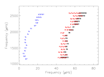
Figure 3: Echelle diagram built from the fitted frequencies for a large separation of 85 $\mu$Hz. The error boxes indicate the 1$\sigma$ (68% confidence) interval.

Degree	Frequency	1$\sigma$	2$\sigma$	Height/Noise
$l$	($\mu$Hz)	interval	interval	ratio
0	1206.25	+2.23/-5.57	+3.92/-7.26	0.6
0	1288.97	+1.25/-0.90	+3.20/-1.97	0.7
0	1373.34	+0.93/-1.16	+1.70/-2.50	1.3
0	1460.14	+0.65/-0.80	+1.22/-2.15	1.4
0	1544.69	+0.85/-0.95	+1.76/-2.05	1.2
0	1631.10	+0.59/-0.69	+1.17/-1.59	2.4
0	1714.49	+1.06/-1.17	+2.00/-2.21	1.9
0	1799.75	+0.84/-1.07	+1.62/-2.62	2.4
0	1884.82	+0.88/-1.26	+1.63/-2.65	2.4
0	1972.73	+0.67/-0.71	+1.30/-1.59	2.3
0	2057.82	+3.22/-1.34	+4.72/-2.24	1.9
0	2147.10	+0.76/-0.83	+1.65/-1.99	1.4
0	2236.46	+2.11/-2.83	+3.85/-5.44	0.9
0	2322.10	+2.22/-3.03	+4.08/-5.64	0.7
0	2408.56	+1.97/-2.33	+3.75/-4.81	0.5
0	2495.76	+3.34/-3.21	+7.00/-6.23	0.3
0	2579.85	+4.70/-3.29	+7.61/-10.7	0.3
1	1161.54	+0.85/-0.91	+1.67/-2.25	0.6
1	1244.63	+1.02/-1.17	+2.39/-2.66	0.7
1	1328.34	+0.70/-0.65	+1.40/-1.26	1.2
1	1414.93	+0.57/-0.58	+1.22/-1.28	1.4
1	1500.54	+0.70/-0.78	+1.36/-1.62	1.2
1	1586.62	+0.48/-0.49	+0.98/-1.02	2.3
1	1670.48	+0.57/-0.58	+1.16/-1.23	1.9
1	1755.30	+0.51/-0.53	+1.06/-1.05	2.3
1	1840.68	+0.49/-0.50	+0.98/-1.02	2.3
1	1928.13	+0.50/-0.51	+1.00/-1.05	2.3
1	2014.38	+0.54/-0.54	+1.07/-1.09	1.8
1	2101.58	+0.67/-0.72	+1.42/-1.56	1.4
1	2190.81	+0.90/-0.90	+1.88/-1.92	0.8
1	2277.89	+1.16/-1.14	+2.33/-2.37	0.7
1	2362.76	+1.61/-1.61	+3.39/-3.48	0.5
1	2450.35	+2.26/-2.71	+4.58/-7.01	0.3
1	2539.49	+1.50/-4.35	+3.24/-11.2	0.3
2	1199.91	+4.08/-5.04	+8.77/-11.3	0.6
2	1287.24	+3.51/-3.77	+7.53/-8.65	0.7
2	1369.60	+2.48/-3.11	+5.25/-7.79	1.3
2	1455.42	+2.33/-1.94	+5.49/-4.07	1.4
2	1541.54	+3.07/-4.47	+5.94/-9.48	1.2
2	1626.30	+2.79/-3.00	+5.16/-6.17	2.4
2	1712.67	+2.83/-2.44	+5.23/-4.75	1.9
2	1794.39	+2.73/-2.10	+6.47/-3.91	2.4
2	1881.83	+2.70/-2.02	+5.27/-4.08	2.4
2	1965.19	+2.01/-1.74	+4.78/-3.55	2.3
2	2060.22	+2.88/-5.17	+4.57/-7.40	1.9
2	2140.32	+3.25/-2.67	+7.02/-5.08	1.4
2	2230.68	+5.10/-2.91	+9.99/-5.89	0.9
2	2316.86	+4.35/-3.35	+9.06/-8.24	0.7
2	2403.52	+3.97/-4.56	+7.77/-11.1	0.5
2	2491.50	+4.96/-5.16	+10.3/-11.2	0.3
2	2576.51	+5.03/-7.94	+9.92/-18.6	0.3

Table 1: Frequencies of the fitted modes. The 1 and 2-$\sigma$ intervals correspond to confidence levels of 68% and 95%, respectively.

Figure 4: Widths of the fitted modes, with 1$\sigma$ error bars

.

4 Conclusion

The two CoRoT observation runs on the star HD49933 – the first 60-day run, and the more recent longer run – have now provided enough data to resolve the identification of modes in the oscillation spectrum at a very high confidence level. This identification relied on several independent analyses. The new data have also allowed us to improve the precision in the mode parameters, with fractional improvements being in the range from 40 % to 70 % depending on the parameter. It is now possible to determine precise mode frequencies for $l$=0 and 1 modes. The $l$=2 mode parameters are more difficult to estimate because of the overlap with the stronger, neighbouring $l$=0 modes. The widths and amplitudes of the modes are well determined, as is the inclination angle of the star. The rotational frequency splitting remains the only mode parameter that is poorly constrained. However, it is clearly much higher than the solar value, and similar or larger in size to the inverse of the surface rotation period. In summary, this new information on the acoustic oscillations of HD49933 now opens the possibility for detailed seismic modeling of the star.

Figure 6: Amplitude ($\sqrt{\pi H\Gamma}$ with $H$ the height and $\Gamma$ the width) of the $l\,=\,0$ fitted modes, with 1$\sigma$ error bars.

Degree	Amplitude	1$\sigma$	Width	1$\sigma$
$l$	(ppm)	interval	($\mu$Hz)	interval
0	1.49	+0.22/-0.22	3.21	+2.19/-1.34
0	2.12	+0.26/-0.24	6.04	+3.60/-2.42
0	2.21	+0.16/-0.16	3.79	+1.12/-0.93
0	2.31	+0.18/-0.17	3.90	+1.39/-1.01
0	2.70	+0.17/-0.17	6.59	+1.97/-1.55
0	3.14	+0.16/-0.15	4.66	+0.99/-0.89
0	3.36	+0.15/-0.15	6.94	+1.23/-1.08
0	3.72	+0.15/-0.15	7.06	+1.11/-1.01
0	3.29	+0.14/-0.14	5.72	+0.90/-0.82
0	3.13	+0.15/-0.14	5.52	+1.10/-1.02
0	2.90	+0.14/-0.14	6.05	+1.21/-1.05
0	2.62	+0.14/-0.14	6.61	+1.69/-1.40
0	2.28	+0.14/-0.15	8.52	+2.14/-1.81
0	2.18	+0.15/-0.15	9.40	+2.48/-2.02
0	1.99	+0.16/-0.16	11.0	+3.36/-2.64
0	1.63	+0.19/-0.19	12.7	+6.71/-4.21
0	1.22	+0.22/-0.22	7.52	+8.72/-4.32
1	1.82	+0.26/-0.28	3.21	+2.19/-1.34
1	2.58	+0.31/-0.30	6.04	+3.60/-2.42
1	2.70	+0.19/-0.20	3.79	+1.12/-0.93
1	2.82	+0.22/-0.21	3.90	+1.39/-1.01
1	3.30	+0.21/-0.21	6.59	+1.97/-1.55
1	3.83	+0.19/-0.19	4.66	+0.99/-0.89
1	4.10	+0.19/-0.19	6.94	+1.23/-1.08
1	4.54	+0.18/-0.18	7.06	+1.11/-1.01
1	4.01	+0.17/-0.17	5.72	+0.90/-0.82
1	3.82	+0.18/-0.17	5.52	+1.10/-1.02
1	3.54	+0.16/-0.17	6.05	+1.21/-1.05
1	3.19	+0.18/-0.18	6.61	+1.69/-1.40
1	2.78	+0.17/-0.18	8.52	+2.14/-1.81
1	2.66	+0.18/-0.18	9.40	+2.48/-2.02
1	2.43	+0.19/-0.20	11.0	+3.36/-2.64
1	1.99	+0.23/-0.23	12.7	+6.71/-4.21
1	1.49	+0.28/-0.27	7.52	+8.72/-4.32
2	1.09	+0.16/-0.16	3.21	+2.19/-1.34
2	1.54	+0.19/-0.18	6.04	+3.60/-2.42
2	1.61	+0.12/-0.12	3.79	+1.12/-0.93
2	1.68	+0.13/-0.12	3.90	+1.39/-1.01
2	1.97	+0.13/-0.12	6.59	+1.97/-1.55
2	2.28	+0.12/-0.11	4.66	+0.99/-0.89
2	2.44	+0.11/-0.11	6.94	+1.23/-1.08
2	2.71	+0.11/-0.11	7.06	+1.11/-1.01
2	2.39	+0.10/-0.10	5.72	+0.90/-0.82
2	2.28	+0.11/-0.10	5.52	+1.10/-1.02
2	2.11	+0.10/-0.10	6.05	+1.21/-1.05
2	1.91	+0.10/-0.10	6.61	+1.69/-1.40
2	1.66	+0.10/-0.11	8.52	+2.14/-1.81
2	1.59	+0.11/-0.11	9.40	+2.48/-2.02
2	1.45	+0.12/-0.12	11.0	+3.36/-2.64
2	1.19	+0.14/-0.14	12.7	+6.71/-4.21
2	0.89	+0.16/-0.16	7.52	+8.72/-4.32

Table 2: Amplitudes and widths of the fitted modes. The 1-$\sigma$ intervals correspond to confidence levels of 68%.

Figure 7: Lightcurves of HD49933 for the 60-day long initial run (left) and the 137-day long run (right)

Figure 9: Mean (upper and lower) 1$\sigma$ error bars for the frequencies of $l$=0 (triangles), $l$=1 (diamonds) and $l$=2 (crosses) modes, showing the decreasing precision on the frequencies from $l$=1 to $l$=2 modes.