Obtaining supernova directional information using the neutrino matter oscillation pattern

Abstract

A nearby core collapse supernova will produce a burst of neutrinos in several detectors worldwide. With reasonably high probability, the Earth will shadow the neutrino flux in one or more detectors. In such a case, for allowed oscillation parameter scenarios, the observed neutrino energy spectrum will bear the signature of oscillations in Earth matter. Because the frequency of the oscillations in energy depends on the pathlength traveled by the neutrinos in the Earth, an observed spectrum contains also information about the direction to the supernova. We explore here the possibility of constraining the supernova location using matter oscillation patterns observed in a detector. Good energy resolution (typical of scintillator detectors), well known oscillation parameters, and optimistically large (but conceivable) statistics are required. Pointing by this method can be significantly improved using multiple detectors located around the globe. Although it is not competitive with neutrino-electron elastic scattering-based pointing with water Cherenkov detectors, the technique could still be useful.

I Introduction

The core collapse of a massive star leads to emission of a short, intense burst of neutrinos of all flavors. The time scale is tens of seconds and the neutrino energies are in the range of a few tens of MeV. Several detectors worldwide, both current and planned for the near future, are sensitive to a core collapse burst within the Milky Way or slightly beyond Scholberg (2007).

The first electromagnetic radiation is not expected to emerge from the star for hours, or perhaps even a few days. Therefore any directional information that can be extracted from the neutrino signal will be advantageous to astronomers who can use such information to initiate a search for the visible supernova. We note that not every core collapse may produce a bright supernova: some supernovae may be obscured, and some core collapses may produce no supernova at all, in which case directional information will aid the search for a remnant.

The possibility of using the neutrinos themselves to point back to the supernova has been explored in the literature Beacom and Vogel (1999); Tomas et al. (2003). Triangulation based on relative timing of neutrino burst signals was also considered in Beacom and Vogel (1999); however available statistics, as well as considerable practical difficulties in prompt sharing of information, makes time triangulation more difficult. Leaving aside the possibility of a TeV neutrino signal Tomas et al. (2003) (which would likely be delayed), the most promising way of using the neutrinos to point to a supernova is via neutrino-electron elastic scattering: neutrinos interacting with atomic electrons scatter their targets within a cone of about 25^∘ with respect to the supernova direction. The quality of pointing goes as $\sim N^{-1/2}$, where $N$ is the number of elastic scattering events. In water and scintillator detectors, neutrino-electron elastic scattering represents only a few percent of the total signal, which is dominated by inverse beta decay $\mathrm{bar}{\nu}_{e}+p\rightarrow n+e^{+}$, for which anisotropy is weak Vogel and Beacom (1999). Furthermore the directional information in the elastic scattering signal is available only for water Cherenkov detectors, for which direction information is preserved via the Cherenkov cone of the scattered electrons. Taking into account the near-isotropic background of non-elastic scattering events Tomas et al. (2003), a Super-K-like detector Ikeda et al. (2007) (22.5 kton fiducial volume) will have 68% (90%) C.L. pointing of about 6^∘ (8^∘) for a 10 kpc supernova; this could improve to $<1^{\circ}$ for next-generation Mton-scale water detectors. Long string water detectors Halzen et al. (1996) do not reconstruct supernova neutrinos event-by-event and so cannot use this channel for pointing. Scintillation light is nearly isotropic and so scintillation detectors have very poor directional capability, although there is potentially information in the relative positions of the inverse beta decay positron and neutron vertices , and some novel scintillator directional techniques are under development Watanabe (2009).

We consider here a new possibility: detectors with sufficiently good energy resolution will be able to obtain directional information by observing the effects of neutrino oscillation on the energy spectrum of the observed neutrinos, assuming that oscillation parameters are such that matter oscillations are present. Although not competitive with elastic scattering, some directional information can be obtained even in a single detector (unlike for time triangulation). Combinations of detectors at different locations around the globe may yield fairly high quality information.

II Determining the Direction with Earth Matter Effects

Supernova neutrinos traversing the Earth’s matter before reaching a detector will experience matter-induced oscillations, depending on the values of the MNS matrix parameters  Dighe and Smirnov (2000); Lunardini and Smirnov (2001); Takahashi and Sato (2002); Lunardini and Smirnov (2003); Dighe et al. (2003, 2004). Whether or not there will be an Earth matter effect depends on currently-unknown mixing parameters, $\theta_{13}$ and the mass hierarchy: matter oscillation will occur for both $\nu_{e}$ and $\mathrm{bar}{\nu}_{e}$ for values of $\sin^{2}\theta_{13}\mathrel{\hbox to0.0pt{\raisebox{1.29167pt}{$<$}\hss}\raisebox{-2.58334pt}{$\sim$}}10^{-5}$, for normal but not inverted hierarchy; if $\theta_{13}$ is relatively large, $\sin^{2}\mathrel{\hbox to0.0pt{\raisebox{1.29167pt}{$>$}\hss}\raisebox{-2.58334pt}{$\sim$}}10^{-3}$, then matter oscillation occurs for $\mathrm{bar}{\nu}_{e}$ but not $\nu_{e}$ for either hierarchy Dasgupta et al. (2008); Dighe (2008). The frequency of the oscillation in $L/E$, where $E$ is the neutrino energy and $L$ is the neutrino pathlength in Earth matter, depends on now fairly well-known mixing parameters. Therefore, the oscillation pattern in neutrino energy $E$ measured at a single detector contains information about the pathlength $L$ traveled through the Earth matter. If the pathlength $L$ is known, one knows that supernova is located somewhere on a ring on the sky corresponding to this pathlength. If another pathlength is measured at a different location on the globe, the location can be further constrained to the intersection of the allowed regions.

A Fourier transform of the inverse-energy distribution Dighe et al. (2003) of the observed neutrinos will yield a peak if oscillations are present. References Dighe et al. (2003) and Dighe et al. (2004) explore the conditions under which peaks are observable with a view to obtaining information about the oscillation parameters. The authors assume that the direction of the supernova, and hence the pathlength through the Earth, is known. Here we turn the argument around: we assume that oscillation parameters are such that the matter effects do occur and can be identified, and that enough is known about MNS parameters to extract information about $L$ and hence about supernova direction from the data. A similar idea to determine possible georeactor location from the oscillated spectrum was explored in reference Dye (2009). We note that by the time a nearby supernova happens, the hierarchy and whether $\theta_{13}$ is large or small may in fact be known from long-baseline and reactor experiments. With reasonably high probability Mirizzi et al. (2006), the Earth will shadow the supernova in at least one detector. We note that lack of observation of a matter peak in the inverse-energy transform (assuming there should be one) gives some direction information as well: if no peak is present, one can infer that the supernova is overhead at a given location. If the hierarchy and value of $\theta_{13}$ are already known with sufficient precision at the time of the supernova, we should know in advance whether or not a peak in the $k$ distribution should appear; otherwise, its appearance for at least one detector location may answer the question.

III Evaluation of the Concept in Idealized Scenarios

To evaluate the general feasibility of this concept we make several simplifying assumptions. We consider only inverse beta decay in large water Cherenkov and liquid scintillator detectors (we ignore the presence of other interactions, which should be a small correction; some of them can be tagged) . We will first consider a detector with perfect energy resolution, and then consider resolutions more typical of real water Cherenkov and scintillator detectors.

We borrow some of the assumptions and notation of reference Dighe et al. (2003). We assume a neutrino interaction cross-section proportional to $E^{2}$, perfect detection efficiency above threshold and no background. We assume a “pinched” neutrino spectrum of the form: $F_{0}=\frac{\phi_{0}}{E_{0}}\frac{(1+\alpha)^{1+\alpha}}{\Gamma\left(1+\alpha\right)}\left(\frac{E}{E_{0}}\right)^{\alpha}\mathrm{e}^{-\left(\alpha+1\right)\frac{E}{E_{0}}}$, where $E_{0}$ is the average neutrino energy. We choose parameters $\alpha=3$, average energies for the flavors $E_{\mathrm{bar}{\nu}_{e}}=$15\text{\,}\mathrm{MeV}$$ and $E_{\mathrm{bar}{\nu}_{x}}=$18\text{\,}\mathrm{MeV}$$, and $\frac{\phi_{\mathrm{bar}{\nu}_{e}}}{\phi_{\mathrm{bar}{\nu}_{x}}}=0{.}8$. These parameters correspond to the “Garching” model Raffelt et al. (2003). We ignore for this study “spectral splits” (e.g. Dasgupta et al. (2009)) or other features which will introduce additional Fourier components. We assume that there are no non-standard neutrino interactions or other exotic effects that modify the spectra.

The oscillation probabilities have been computed by numerical solution of the matter oscillation equations Wendell (2009) using these vacuum parameters and the full PREM Earth density model Dziewonski and Anderson (1981). Between neighboring radial points in the model the matter density is taken to be constant such that the three-neutrino transition amplitude may be computed following the methods outlined in Barger et al. (1980). The final amplitude is the product of all amplitudes across the matter slices along the neutrino’s trajectory. The initial flux of neutrinos is taken to arrive at the Earth as pure mass states such that the detection probability is taken according to the probability of a neutrino being $\mathrm{bar}{\nu}_{e}$ flavor when it reaches the detector. The oscillation parameters were chosen to be $\sin^{2}{2\theta_{12}}=0{.}87$, $\sin^{2}{2\theta_{13}}=0$, $\sin^{2}{2\theta_{23}}=1{.}0$, $\Delta m_{12}^{2}=7{.}6\times$10^{-5}\text{\,}\mathrm{eV}^{2}$$, and $\Delta m_{23}^{2}=2{.}4\times$10^{-3}\text{\,}\mathrm{eV}^{2}$$.

III.1 Perfect Energy Resolution

The spectrum of inverse beta decay events, integrated over time, is shown in Fig. 1. Fig. 1 shows on the bottom the “inverse-energy” spectrum, where the inverse-energy parameter $y$ is defined as $y=\frac{$12{.}5\text{\,}\mathrm{MeV}$}{E}$. Fig. 2 shows the Earth matter modulation of the spectrum, for $L=6,000$ km. Shown on the bottom is the modulation in inverse-energy, for which the peaks are evenly spaced.

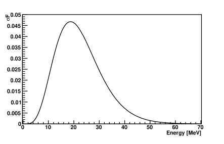
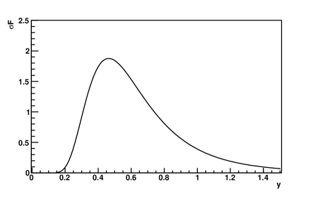
Figure 1: Top: assumed neutrino event spectrum without oscillations. Bottom: inverse-energy distribution.

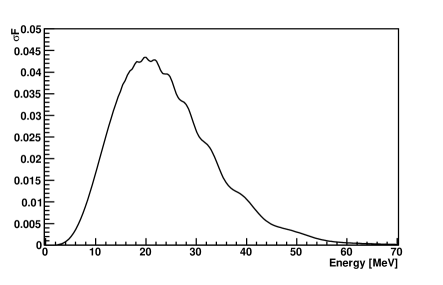
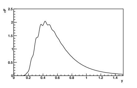
Figure 2: Top: assumed neutrino event spectrum with matter oscillations for $L=6,000$ km. Bottom: inverse-energy distribution with matter oscillations.

The Fourier transform of the detected inverse-energy spectrum is $g(k)=\int_{-\infty}^{\infty}f(y)e^{iky}dy$. The power spectrum $G_{\sigma F}(k)=|g(k)|^{2}$ assuming perfect energy resolution is shown in Fig. 3, for no matter oscillation on the top and for matter oscillation on the bottom, assuming pathlength $L=6,000$ km. The power spectra are generated from the normalized inverse-energy distributions for which $\int_{0}^{\infty}\sigma F(y)\mathrm{d}y=1$. Thus the power spectra are normalized so that $G_{\sigma F}(0)=1$. Fig. 4 shows the power spectra for several values of $L$, illustrating how the peak moves to higher $k$ values as the pathlength increases. For pathlengths such that the neutrinos traverse the Earth core ($L>10,700$ km), additional peaks are present in the spectrum Dighe et al. (2004). There is no observable peak for $L$ less than about 2500 km, for which the neutrinos are no longer traversing much high-density matter.

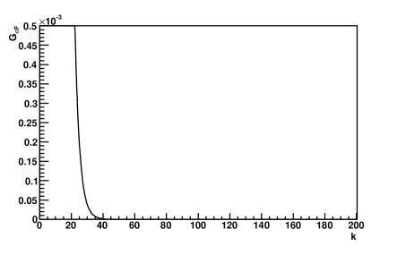
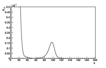
Figure 3: Inverse-energy power spectrum without (top) and with (bottom) matter oscillations.

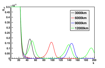
Figure 4: Examples of inverse-energy power spectra for several pathlengths.

Fig. 5 shows now the effect of finite statistics, for a simulated supernova with 10,000 events and one with 60,000 events. The finite statistics result in a background for the main peak(s) in the power spectrum. For most of the following, we consider a rather optimistically large (but not unthinkable) 60,000 event signal, which would correspond to a supernova at a distance of about 5 kpc observed with a 50 kton detector.

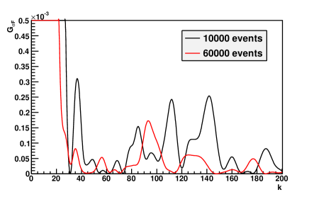
Figure 5: Examples of inverse-energy power spectra for perfect energy resolution but finite statistics. Both lines show $L=6000$ km.

III.1.1 Method for Determining Directional Information

If one measures $k_{\rm peak}$, the position of the largest peak in the power spectrum, for a supernova signal, one can in principle determine the pathlength traveled by the neutrino in the Earth. We use a simple Neyman construction method Amsler et al. (2008) to estimate the quality of directional information.

We first find the position of the largest peak in $k$ as a function of pathlength $L$, assuming perfect energy resolution but finite statistics. To find the peak in the power spectrum, we first set a lower threshold of $k=40$ and an upper threshold of $k=210$. Below that threshold, the peak merges with the low $k$ peak (corresponding to the unoscillated spectrum) and can no longer be identified. Peaks beyond $k=210$ would correspond to distances greater than the diameter of the Earth. For each $k$ within that range we then evaluate the integral from $k-\Delta k/2$ to $k+\Delta k/2$ which corresponds to the area under the peak. We take the $k$ for which this value is highest as the peak in the spectrum. We chose $\Delta k=4$. Even though Fig. 4 suggests that peaks can be wider than that, we found more fluctuation in the peak’s position for higher $\Delta k$ when taking finite energy resolution into account, especially for small distances ($L<4000$ km). Fig. 6 shows that the value of $k_{\rm peak}$ is clearly correlated with pathlength $L$; for distances less than about 2000 km, for which the neutrinos do not undergo matter oscillations, it represents mainly random noise. The multiple peak structure for neutrinos passing through the core is clearly visible for $L>10,700\leavevmode\nobreak\$km. We note that the height of the largest peak also contains information about $L$, as do the secondary peak positions, if such exist.

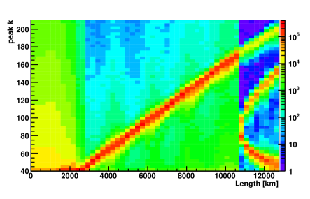
Figure 6: Distribution of the position of the maximum peak in $k$ as a function of matter-traversed pathlength $L$, assuming perfect energy resolution. There are 500,000 simulated supernovae per $L$, each with 60,000 events.

Given a particular measurement of $k_{\rm peak}$, one can then determine a range of distances $L$ allowed, making use of the Neyman construction shown in Fig. 7. To ensure contiguous regions in $k$ we drop regions that contribute less than 3% to the final Neyman construction and increase existing regions instead so that the total covered area is 68% or 90%. The range in $L$ values can then be mapped to an allowed region on the sky. We have checked explicitly that the statistical coverage is as expected.

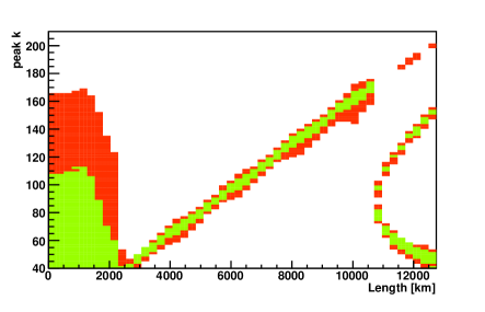
Figure 7: Neyman construction for $k_{\rm peak}$ and $L$: for a given measured $k_{\rm peak}$ one reads off a range of allowed $L$ values. The green area shows the 68% confidence region and the red area the 90% one.

Fig. 8 shows an example Hammer projection sky map in equatorial coordinates showing 90% C.L. allowed regions for an assumed true supernova direction (indicated by a star) of R.A.$=20^{h}$ and decl.$=-60^{\circ}$ (occurring at 0:00 GMST), for assumed perfect energy resolution and statistics of 60,000 events.

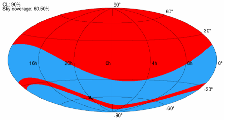
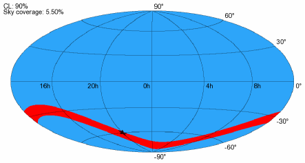
Figure 8: Example Hammer projection skymaps in equatorial coordinates, showing 90% C. L. allowed regions on the sky for a supernova at the position indicated by a star. A 60,000 neutrino event signal measured in Finland with perfect energy resolution is assumed. The top plot shows the allowed region without taking into account peak height; the bottom plot takes into account peak height information.

Fig. 9 shows the distribution of fractional sky coverage for perfect energy resolution. The distribution is bimodal, because the $L<2500$ km possibility (corresponding to large fractional sky coverage) is often not excluded at 90% in the Neyman construction. Fig. 10 shows the average sky coverage vs. declination of the supernova, averaged over 24h of right ascension, for a detector located in Finland ($63{.}66^{\circ}$ N, $26{.}04^{\circ}$ E).

If we incorporate also information about the height of the largest peak $h$ into a Neyman construction, for long pathlengths we can remove the possibility of a short-pathlength overhead supernova, and improve the pointing quality significantly. Fig. 11 shows the correlation between peak heights and $L$. Figs. 8 (bottom) and 10 show the effect of incorporating this information. Subsequent plots will assume use of both Fourier peak position and height information.

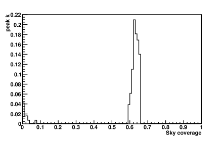
Figure 9: Histogram of fractional sky coverages for the 90% C.L. region, assuming perfect energy resolution in a single detector, using $k_{\rm peak}$ information only, for the example configuration of Fig. 8.

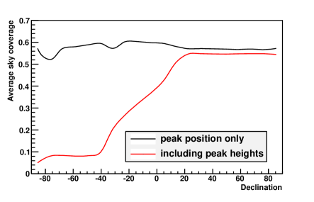
Figure 10: Sky coverage averaged over right ascension as a function of declination, for a single detector. The black line just takes into account the peak position, whereas the red line includes also the height of the peak. In total, 83,500 supernovae, evenly distributed over declination, have been simulated for both lines.

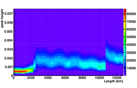
Figure 11: Distribution of the heights of the maximum peak in $k$ as a function of matter-traversed pathlength $L$, assuming perfect energy resolution. There are 500,000 simulated supernovae per $L$, each with 60,000 events.

III.1.2 Combining Detectors

Clearly, having several detectors around the globe observing the neutrino burst will improve the measurement. If each of the detectors could select a single $L$, an observation with two detectors will produce two allowed regions where the rings on the sky overlap, and a third observation will narrow it down to one spot. However because more than one $L$ region may be allowed for a given detector, the combination can include multiple regions.

For the multiple detector case, we make the Neyman construction for 100,000 randomly chosen $(k_{1};h_{1},k_{2};h_{2},\ldots)$-tuples only (with 100 bins in $k_{\rm peak}$ and height for each detector) in order to compute it in a reasonable amount of time. In this case the smoothing procedure described above is not applied.

Fig. 12 shows example scenarios involving two and three detectors and Fig. 13 summarizes average quality as a function of declination. Clearly in this idealized situation, combined information is quite good, and the more detectors spread around the globe, the better.

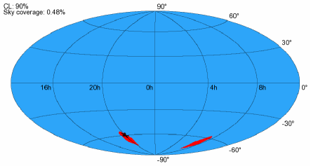
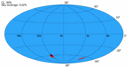
Figure 12: Combined skymaps for detectors with perfect resolution. Top: Two detectors with 60,000 events each. Bottom: Three detectors with 60,000 events each.

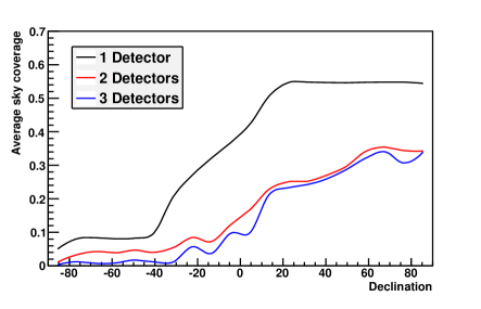
Figure 13: Sky coverage averaged over right ascension as a function of declination, for one, two and three detectors. For one detector 83,500 supernovae have been simulated, for two detectors the number is 2,630 and for three detectors it is 760.

III.2 More Realistic Detectors

Next we will assume a slightly more realistic situation. Imperfect energy resolution will tend to smear out the oscillation pattern and degrade the detectability of the peak in $k$. We estimate the effect of energy resolution by selecting events from the spectrum and smearing their energies according to a Gaussian of the prescribed width. The energy resolution functions used, the same as in reference Dighe et al. (2004), are shown in Fig. 14; one is characteristic of scintillator and one of water Cherenkov detectors. For water Cherenkov we assume a threshold of 5 MeV and for scintillator we assume a threshold of 1 MeV.

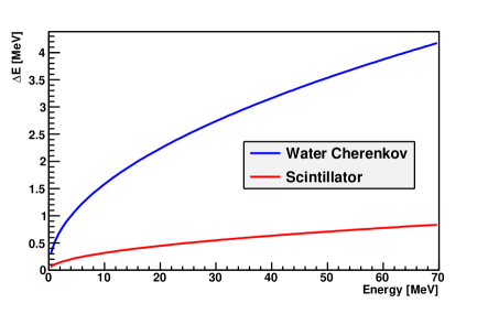
Figure 14: Energy resolution functions used for water and scintillator. $\Delta E$ is the standard deviation $\sigma$ of a Gaussian.

III.2.1 Water Cherenkov Detectors

Fig. 15 shows the distribution of $k_{\rm peak}$ and $L$ for simulated supernovae in a detector with water-Cherenkov-like energy resolution. Fig. 16 shows the same for scintillator.

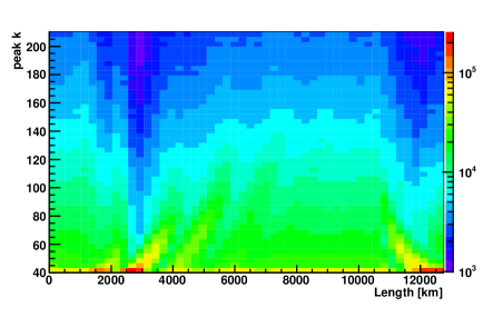
Figure 15: Distribution of the position of the maximum peak in $k$ as a function of matter-traversed pathlength $L$, assuming water Cherenkov energy resolution. There are 500,000 simulated supernovae per $L$, each with 60,000 events.

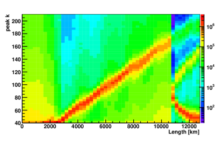
Figure 16: Distribution of the position of the maximum peak in $k$ as a function of matter-traversed pathlength $L$, assuming scintillator energy resolution. There are 5,000,000 simulated supernovae per $L$, each with 60,000 events.

Clearly the water Cherenkov resolution smears the power spectrum information enough to preclude its use for this purpose; furthermore, far superior direction information will come from elastic scattering in a water Cherenkov detector. Therefore we will focus subsequent attention on scintillator detectors, which have significantly better energy resolution and weak intrinsic direct pointing capabilities.

III.2.2 Scintillator Detectors

Existing and near-future scintillator detectors with supernova neutrino detection capabilities are KamLAND Eguchi et al. (2003), LVD Aglietta et al. (1992); Agafonova et al. (2007), Borexino Cadonati et al. (2002) and SNO+ Kraus (2006); these are however probably too small to acquire the large statistics required for this technique. Future scintillator detectors of the tens of kton scale for which this technique could be feasible are LENA Marrodan Undagoitia et al. (2008), to be sited in Finland, and the ocean-based HanoHano Learned et al. (2008).

Fig. 17 shows an example skymap for a scintillator detector located in Finland. Fig. 18 shows average sky coverage vs. declination for three examples of event statistics.

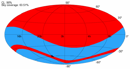
Figure 17: Example scintillator skymaps, for a single detector located in Finland, assuming a 60,000 event signal (top).

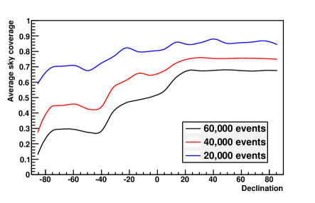
Figure 18: Average scintillator sky coverage vs declination for a single detector located in Finland, for 20,000 event, 40,000 and 60,000 event signals. In total 200,000 supernovae have been simulated for the 60,000 events case and 12,000 and 15,000 for the 20,000 and 40,000 event cases, respectively.

Next we consider the case when multiple detectors are operating: Fig. 19 shows the results of combining the information from two and three scintillator detectors located in Finland, off the coast of Hawaii ($19{.}72^{\circ}$ N, $156{.}32^{\circ}$ W) and South Dakota ($44{.}45^{\circ}$ N, $103{.}75^{\circ}$ W). Fig. 20 shows average sky coverage vs. declination for these configurations.

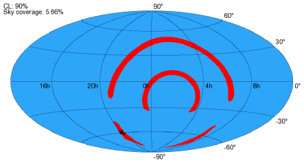
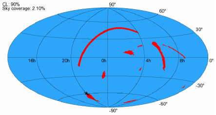
Figure 19: Example scintillator skymaps, for a two (top) and three (bottom) detectors setup, each with a 60,000 events signal per detector.

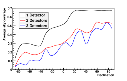
Figure 20: Average scintillator sky coverage vs declination for one, two and three detectors with 60,000 events each. For one detector 200,000 supernovae have been simulated, for two detectors the number is 3,500 and for three detectors it is 1,256.

III.2.3 Incorporating Relative Timing Information

We consider briefly now the possibility of incorporating relative timing information between detectors to break degeneracies in the allowed region(s). A detailed study of the triangulation capabilities for specific neutrino signal and detector models is beyond the scope of this work. We instead do some back-of-the-envelope estimates based on those in reference Beacom and Vogel (1999). For a signal registered in two detectors, the supernova direction can be constrained to a ring on the sky at angle $\theta$ with respect to the line between the detectors, with $\cos\theta=\Delta t/d$ and width $\delta(\cos\theta)\sim\frac{\delta(\Delta t)}{d}$, where $d$ is the distance between the detectors and $\delta(\Delta t)$ is the time shift uncertainty between the pulses. We assume $\delta(\Delta t)\sim 30{\rm\leavevmode\nobreak\ ms}/\sqrt{N_{1}}$, where $N_{1}$ is $\sim$1% of the total signal. A sharp feature in the signal timing could reduce $\delta(\Delta t)$.

Fig. 21 shows an example for two detectors (located in Finland and Hawaii), with the time-triangulated allowed region superimposed: the intersection clearly narrows down the allowed directions.

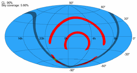
Figure 21: Example two scintillator detector skymap, with estimate of allowed region based on relative timing information superimposed (dark band).

We can imagine also that another, non-scintillator, neutrino detector (or even a gravitational wave detector, e.g. Pagliaroli et al. (2009)) could provide relative timing information as well. For example, IceCube at the South Pole could yield few ms timing Halzen and Raffelt (2009). Fig. 22 shows an example of the intersection of the estimated IceCube plus single scintillator detector time-triangulation allowed region (assuming $\delta(\Delta t)\sim 1\leavevmode\nobreak\$ms) with the single scintillator oscillation pattern region.

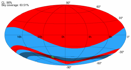
Figure 22: Example single scintillator detector skymap, with estimated allowed region determined from relative timing with the IceCube signal (dark band).

IV Discussion

We have assumed in these idealized scenarios perfect knowledge of oscillation parameters. In practice, imperfect knowledge of the oscillation parameters will create some uncertainties. In particular, the power spectrum peak position is sensitive to the value of $\Delta m^{2}_{12}$; the peak height is sensitive to both $\Delta m^{2}_{12}$ and $\theta_{12}$; $\theta_{13}$ also has an effect on both $k_{\rm peak}$ and $h$. (The oscillation pattern is quite insensitive to the 23 mixing parameters.) Figs. 23 and 24 show the effect on $k_{\rm peak}$ and $h$ values of varying the oscillation parameters within currently allowed ranges Abe et al. (2008).

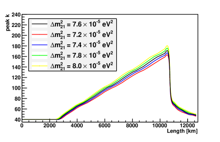
Figure 23: Effect of varying $\Delta m^{2}_{12}$ on the peak position as a function of $L$; in each case other oscillation parameters are held at their nominal values.

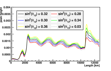
Figure 24: Effect of varying $\theta_{12}$ and $\theta_{13}$ on the peak height as a function of $L$; in each case the other oscillation parameters are held at their nominal values.

From these plots one can infer that $\mathrel{\hbox to0.0pt{\raisebox{1.29167pt}{$<$}\hss}\raisebox{-2.58334pt}{$\sim$}}$1% knowledge of the mixing parameters is desirable. However, one can be quite optimistic that such precision will have been attained by the time a core collapse supernova happens when a large scintillator detector is running.

Another uncertainty that will affect the quality of pointing is that of the density of matter in the Earth. We found only small differences in $k_{peak}$ and $h$ from varying the mantle density by $\pm 3\%$, or from varying the overall density by $\pm 5\%$, but observed some changes in peak pattern for the case of neutrinos passing through the core when varying the core density by $\pm 10\%$.

Many other effects may degrade the quality of direction information that can be obtained using this technique. There may be real spectral features (e.g. “splits”) which introduce additional Fourier components that could mask the peak, and detector imperfections may do the same. We acknowledge also that there may be practical difficulties with the rapid exchange of information between experimenters required for prompt extraction of directional information from multiple detectors. Nevertheless this technique represents an interesting possibility– even half the sky is better than no directional information. The oscillation pattern gives information about direction with even a single detector, and enhances any multiple-detector time-triangulation information. Even if information from only a single detector is available, or if there are significant ambiguities, one can imagine also looking at the intersection of the allowed region with the Galactic plane regions for which supernovae are most likely to occur (Mirizzi et al. (2006)) (perhaps using the known probability distribution as a Bayesian prior) to improve the chances of finding the supernova: see Fig. 25.

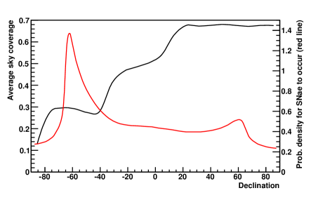
Figure 25: Average scintillator sky coverage vs declination for a single detector in Finland, with the expected probability for supernova occurrence superimposed from reference Mirizzi et al. (2006).

We note that these estimates of pointing quality have been done using a fairly simple technique based on only two parameters characterizing the power spectra. One can imagine employing more sophisticated algorithms, e.g. making use of secondary peaks or matching to a template, and possibly incorporating knowledge of specific detector properties or neutrino flux spectral features. So although real conditions may degrade quality, with this simplified study we have not fully exploited all potentially available information.

As a final note: the technique could in principle work to determine directional information for neutrino signals from other astrophysical sources, such as black hole-neutron star mergers Caballero et al. (2009), assuming sufficient statistics.

V Summary

We have explored a technique by which experiments with good energy resolution can determine information about the direction of a supernova via measurement of the matter oscillation pattern. This method will only work for favorable (but currently allowed) oscillation parameters; it requires large statistics, good energy resolution, and well-known oscillation parameters, and it works best for relatively long neutrino pathlengths through the Earth. The method is especially promising for scintillator detectors. The criteria will be fulfilled in optimistic but not inconceivable scenarios. Combining information from multiple detectors, and possibly incorporating relative timing information, may provide significant improvement. The method is inferior to that using elastic scattering in imaging Cherenkov (or argon time projection chamber) detectors; elastic scattering remains the best bet for pointing to the supernova. However it is possible that a supernova will occur when no such detector is running, in which case one should use whatever directional information can be extracted from the observed signals.