CPHT-092.0909

Heterotic Resolved Conifolds with Torsion,

from Supergravity to CFT

L. Carlevaro^⋄ and D. Israël^♠

^⋄Centre de Physique Théorique, Ecole Polytechnique, 91128 Palaiseau, France

^♠Institut d’Astrophysique de Paris, 98bis Bd Arago, 75014 Paris, France

Abstract

We obtain a family of heterotic supergravity backgrounds describing non-Kähler warped conifolds with three-form flux and an Abelian gauge bundle, preserving $\mathcal{N}=1$ supersymmetry in four dimensions. At large distance from the singularity the usual Ricci-flat conifold is recovered. By performing a $\mathbb{Z}_{2}$ orbifold of the $T^{1,1}$ base, the conifold singularity can be blown-up to a four-cycle, leading to a completely smooth geometry. Remarkably, the throat regions of the solutions, which can be isolated from the asymptotic Ricci-flat geometry using a double-scaling limit, possess a worldsheet cft description in terms of heterotic cosets whose target space is the warped resolved orbifoldized conifold. Thus this construction provides exact solutions of the modified Bianchi identity. By solving algebraically these cfts we compute the exact tree-level heterotic string spectrum and describe worldsheet non-perturbative effects. The holographic dual of these solutions, in particular their confining behavior, and the embedding of these fluxed singularities into heterotic compactifications with torsion are also discussed.

1 Introduction

Heterotic compactifications to four dimensions have acquired over the years a cardinal interest for phenomenological applications, as their geometrical data combined with the specification of a holomorphic gauge bundle have played a major role in recovering close relatives to the mssm or intermediate guts. However, as their type ii counterparts, heterotic Calabi-Yau compactifications are generally plagued with the presence of unwanted scalar degrees of freedom at low-energies.

A fruitful strategy to confront this issue has proven to be the inclusion of fluxes through well-chosen cycles in the compactification manifold. Considerable effort has been successfully invested in engineering such constructions in type ii supergravity scenarii (see [1] for a review and references therein). However, if one is eventually to uncover the quantum theory underlying these backgrounds, warranting their consistency as string theory vacua, or to evade the large-volume limit where supergravity is valid, one has to face the presence of rr fluxes intrinsic to these type ii backgrounds, for which a worldsheet analysis is still lacking.

In this respect, heterotic geometries with nsns three-form and gauge fluxes are more likely to allow for such a description ; the dilaton not being stabilized perturbatively the worldsheet theory should be amenable to standard cft techniques. The generic absence of large-volume limit in heterotic flux compactifications makes even this appealing possibility a necessity. An attempt in uncovering an underlying worldsheet theory for heterotic flux vacua has been made in [2, 3] by resorting to linear sigma-model techniques. This approach however yields a fully tractable description only in the uv, while the interacting cft obtained in the ir is not known explicitly.

A consistent smooth heterotic compactification requires determining a gauge bundle that satisfies a list of consistency conditions. This sheds yet another light on the appearance of non-trivial Kalb-Ramond fluxes, now understood as the departure, triggered by the choice of an alternative gauge bundle, from the standard embedding of the spin connection into the gauge connection that characterizes Calabi-Yau compactifications. This eventually leads to geometries with torsion. Now, heterotic flux compactifications, although known for a long time (see e.g. [4, 5, 6, 7, 8, 9, 10, 11, 12, 13]) are usually far less understood that their type iib counterparts.

In particular having a non-trivial $\mathcal{H}$-flux threading the geometry results in the metric loosing Kählerity (see [15] for the analysis of $T^{2}$ fibrations over $K3$) and being conformally balanced instead of Calabi-Yau [16, 17, 18]. This proves as a major drawback for the analysis of such backgrounds, as theorems of Kähler geometry (such as Yau’s theorem) do not hold anymore, making the existence of solutions to the tree-level supergravity equations dubious, let alone their extension to exact string vacua. An additional and general complication for heterotic solutions comes from anomaly cancellation, which requires satisfying the Bianchi identity in the presence of torsion. This usually proves notoriously arduous as this differential constraint is highly non-linear. A proof of the existence of a family of smooth solutions to the leading-order Bianchi identity has only appeared recently [19] (see also [15] for an earlier discussion of $T^{2}\times K3$ fibrations, as well as [20, 21, 22] for developments).

Moduli spaces of heterotic compactifications have singularities, that arise whenever the gauge bundle degenerates to ’point-like instantons’, either at regular points or at singular points of the compactification manifold. In the case of $\mathcal{N}=1$ compactifications in six dimensions, the situation is well understood. Point-like instantons at regular points of $K3$ signals the appearance of non-perturbative $Sp(k)$ gauge groups in the case of $Spin(32)/\mathbb{Z}_{2}$ [23], while for $E_{8}\times E_{8}$ one gets tensionless bps strings [24], leading to interacting scfts. In both cases, the near-core ’throat’ geometry of small instantons is given by the heterotic solitons of Callan, Harvey and Strominger [25] (called thereafter chs), that become heterotic five-branes in the point-like limit. In the case of four-dimensional $\mathcal{N}=1$ cy₃ compactifications, let alone torsional vacua, the situation is less understood. For a particular class of cy₃ which are $K3$ fibrations, one can resort to the knowledge of the six-dimensional models mentioned above – advocating an ’adiabatic’ argument – in order to understand the physics in the vicinity of such singularities [26, 27].

Recently, a study of heterotic flux backgrounds, supporting an Abelian line bundle, has been initiated [28]. In a specific double-scaling limit of these torsional vacua, the corresponding worldsheet non-linear sigma model has been shown to admit a solvable cft description, belonging to a particular class of gauged wzw models, whose partition function and low-energy spectrum could be established. In the double-scaling limit where this cft description emerges, one obtains non-compact torsional manifolds, that can be viewed as local models of heterotic flux compactifications, in the neighborhood of singularities supporting Kalb-Ramond and magnetic fluxes. In analogy with the Klebanov–Strassler (ks) solution [29], which plays a central role in understanding type iib flux backgrounds [30], these local models give a good handle on degrees of freedom localized in the ’throat’ geometries.

The solutions we are considering correspond to the near-core geometry of ’small’ gauge instantons sitting on geometrical singularities, and their resolution. Generically, the torsional nature of the geometry can come solely from the local backreaction of the gauge instanton (as for the chs solution that corresponds to a gauge instanton on a $K3$ manifold that is globally torsionless), or thought of being part of a globally torsional compactification. From the point of view of the effective four- or six-dimensional theory, these solutions describe (holographically) the physics taking place at non-perturbative transitions of the sort discussed above, or in their neighborhood in moduli space.

In the present work we concentrate on heterotic flux backgrounds preserving $\mathcal{N}=1$ supersymmetry in four dimensions. More specifically we consider codimension four conifold singularities [31], supplemented by a non-standard gauge bundle which induces non-trivial torsion in the $SU(3)$ structure connection. For definiteness we opt for $Spin(32)/\mathbb{Z}_{2}$ heterotic string theory. The Bianchi identity is satisfied for an appropriate Abelian bundle, which solves the differential constraint in the large charge limit, where the curvature correction to the identity becomes sub-dominant. Subsequently, numerical solutions to the $\mathcal{N}=1$ supersymmetry equations [4] can be found, which feature non-Kähler spaces corresponding to warped torsional conifold geometries with a non-trivial dilaton. At large distance from the singularity, their geometry reproduces the usual Ricci-flat conifold, while in the bulk we observe a squashing of the $T^{1,1}$ base, as the radius of its $S^{1}$ fiber is varying.

The topology of this class of torsional spaces allows to resolve the conifold singularity by a blown-up $\mathbb{C}P^{1}\times\mathbb{C}P^{1}$ four-cycle, provided we consider a $\mathbb{Z}_{2}$ orbifold of the original conifold space, that avoids the potential bolt singularity. In contrast, in the absence of the orbifold only small resolution by a blown-up two-cycle or deformation to a three-cycle remain as possible resolutions of the singularity. The specific de-singularisation we are considering here is particularly amenable to heterotic or type I constructions, as it leads to a normalizable harmonic two-form which can support an extra magnetic gauge flux (type iib conifolds with blown-up four-cycles and D3-branes were discussed in [32, 33, 34]). The numerical supergravity solutions found in this case are perfectly smooth everywhere, and the string coupling can be chosen everywhere small, while in the blow-down limit the geometrical singularity is also a strong coupling singularity.

In the regime where the blow-up parameter $a$ is significantly smaller (in string units) than the norm of the vectors of magnetic charges, one can define a sort of ’near-horizon’ geometry of this family of solutions, where the warp factor acquires a power-like behavior. This region can be decoupled from the asymptotic Ricci-flat region by defining a double scaling limit [28] which sends the asymptotic string coupling $g_{s}$ to zero, while keeping the ratio $g_{s}/a^{2}$ fixed in string units.

In this limit we are able to find an analytical solution (that naturally gives an accurate approximation of the asymptotically Ricci-flat solution in the near-horizon region of the latter), where the dilaton becomes asymptotically linear, while the effective string coupling, defined at the bolt, can be set to any value by the double-scaling parameter.

Remarkably, the double-scaling limit of this family of torsional heterotic backgrounds admits a solvable worldsheet cft description, which we construct explicitly in terms of an asymmetric gauged wzw model, which is parametrised by the two vectors $\vec{p}$ and $\vec{q}$ (dubbed hereafter ’shift vectors’) giving the embedding of the two magnetic fields in the Cartan subalgebra of $\mathfrak{so}(32)$. We establish this correspondence by showing that, integrating out classically the worldsheet gauge fields, one obtains a non-linear sigma-model whose background fields reproduce the warped resolved orbifoldized conifold with flux. This result generalizes the cft description for heterotic gauge bundles over Eguchi-Hanson (eh) space or eh$\times T^{2}$ we achieved in a previous work [28].

The existence of a worldsheet cft for this class of smooth conifold solutions first implies that these backgrounds are exact heterotic string vacua to all orders in $\alpha^{\prime}$, once included the worldsheet quantum corrections to the defining gauged wzw models. This can be carried out by using the method developed in [36, 37, 38] and usually amounts to a finite correction to the metric. Furthermore, this also entails that the Bianchi identity is exactly satisfied even when the magnetic charges are not large, at least in the near-horizon regime.

Then, by resorting to the algebraic description of coset cfts, we establish the full tree-level string spectrum for these heterotic flux vacua, with special care taken in treating both discrete and continuous representations corresponding respectively to states whose wave-functions are localized near the singularity, and to states whose wave-functions are delta-function normalizable.

Dealing with arbitrary shift vectors $\vec{p}$ and $\vec{q}$ in full generality turns out to be technically cumbersome, as the arithmetical properties of their components play a role in the construction. We therefore choose to work out the complete solution of the theory for a simple class of shift vectors that satisfy all the constraints. We compute the one-loop partition function in this case (which vanishes thanks to space-time supersymmetry), and study in detail the spectrum of localized massless states.

In addition, the cft construction given here provides information about worldsheet instanton corrections. These worldsheet non-perturbative effects are captured by Liouville-like interactions correcting the sigma-model action, that are expected to correspond to worldsheet instantons wrapping one of the $\mathbb{C}P^{1}$s of the four-cycle. We subsequently analyze under which conditions the Liouville potentials dictated by the consistency of the cft under scrutiny are compatible with the whole construction (in particular with the orbifold and gso projections). This allows to understand known constraints in heterotic supergravity vacua (such as the constraint on the first Chern class of the gauge bundle) from a worldsheet perspective.

Finally, considering that in the double-scaling limit we mentioned above these heterotic torsional vacua feature an asymptotically linear dilaton, we argue that they should admit a holographic description [39]. The dual theory should be a novel kind of little string theory, specified by the shift vector $\vec{p}$ in the uv, flowing at low energies to a four-dimensional $\mathcal{N}=1$ field theory. This theory sits on a particular branch in its moduli space, corresponding to the choice of second shift vector $\vec{q}$, and parametrized by the blow-up mode. We use the worldsheet cft description of the gravitational dual in order to study the chiral operators of this four-dimensional theory, thereby obtaining the R-charges and representations under the global symmetries for a particular class of them. From the properties of the heterotic supergravity solution, we argue that the $Spin(32)/\mathbb{Z}_{2}$ blown-up backgrounds seem to be confining, while for the $E_{8}\times E_{8}$ theory the blow-down limit gives an interacting superconformal field theory.

This work is organized as follows. Section 2 contains a short review of supersymmetric heterotic flux compactifications. In section 3 we obtain the heterotic supergravity backgrounds of interest, featuring torsional smooth conifold solutions. We provide the numerical solutions for the full asymptotically Ricci-flat vacua together with the analytical solution in the double-scaling limit. In addition we study the torsion classes of these solutions and their (non-)Kählerity. In section 4 we discuss the corresponding worldsheet cft by identifying the relevant heterotic gauged wzw model. In section 5 we explicitly construct the complete one-loop partition function and analyze worldsheet non-perturbative effects. Finally in section 6 we summarize our results and discuss two important aspects: the holographic duality and the embedding of these non-compact torsional backgrounds in heterotic compactifications. In addition, some details about the gauged wzw models at hand and general properties of superconformal characters are given in two appendices.

2 $\mathcal{N}$=1 Heterotic vacua with Torsion

In this section we review some known facts about heterotic supergravity and compactifications to four dimensions preserving $\mathcal{N}=1$ supersymmetry. This will in particular fix the various conventions that we use in the rest of this work.

2.1 Heterotic supergravity

The bosonic part of the ten-dimensional heterotic supergravity action reads (in string frame):

$$S=\frac{1}{\alpha^{\prime 4}}\int\mathrm{d}^{10}x\sqrt{-G}e^{-2\Phi}\,\Big{[}R+4|\partial\Phi|^{2}-\frac{1}{2}|\mathcal{H}|^{2}+\frac{\alpha^{\prime}}{4}\big{(}\mbox{Tr}_{\text{V}}|\mathcal{F}|^{2}+\text{tr}|\mathcal{R}_{+}|^{2}\big{)}\Big{]}\,.$$ (2.1)

with the norm of a $p$-form field strength $\mathcal{G}_{[p]}$ defined as $|\mathcal{G}|^{2}=\nicefrac{{1}}{{p!}}\,\mathcal{G}_{M_{1}..M_{p}}\mathcal{G}^{M_{1}..M_{p}}$. The trace of the Yang-Mills kinetic term is taken in the vector representation of $SO(32)$ or $E_{8}\times E_{8}$.

To be in keep with the modified Bianchi identity below (2.3), we have included in (2.1) the leading string correction to the supergravity Lagrangian. It involves the generalized curvature two-form $\mathcal{R}(\Omega_{+})^{A}_{\phantom{A}B}$ built out of a Lorentz spin connexion $\Omega_{+}$ that incorporates torsion, generated by the presence of a non-trivial nsns three-form flux:

$$\Omega^{\phantom{\pm}A}_{\pm\,\phantom{A}B}=\omega^{A}_{\phantom{A}B}\pm\tfrac{1}{2}\mathcal{H}^{A}_{\phantom{A}B}\,.$$ (2.2)

In addition to minimizing the action (2.1), a heterotic vacuum has to fulfil the generalized Bianchi identity:

$$\mathrm{d}\mathcal{H}_{[3]}=8\alpha^{\prime}\pi^{2}\Big{[}\text{ch}_{2}\big{(}V\big{)}-p_{1}\big{(}\mathcal{R}(\Omega_{+})\big{)}\Big{]}\,,$$ (2.3)

here written in terms of the first Pontryagin class of the tangent bundle and the second Chern character of the gauge bundle $V$. The second topological term on the right hand side is the leading string correction to the Bianchi identity required by anomaly cancellation [40], and mirrors the one-loop correction on the lhs of (2.1).

By considering gauge and Lorentz Chern-Simons couplings, one can now construct an nsns three-form which exactly solves the modified Bianchi identity (2.3):

$$\mathcal{H}_{[3]}=\mathrm{d}\mathcal{B}_{[2]}+\alpha^{\prime}\big{(}\omega_{[3]}^{L}(\Omega_{+})-\omega_{[3]}^{\textsc{ym}}(\mathcal{A})\big{)}\,,$$ (2.4)

thus naturally including tree-level and one-loop corrections, given by:

$$\omega_{[3]}^{\textsc{ym}}(\mathcal{A})=\text{Tr}_{\textsc{v}}\left[\mathcal{A}\wedge\mathrm{d}\mathcal{A}+\tfrac{2}{3}\,\mathcal{A}\wedge\mathcal{A}\wedge\mathcal{A}\right]\,,\qquad\omega_{[3]}^{L}(\Omega_{+})=\text{tr}\left[\Omega_{+}\wedge\mathrm{d}\Omega_{+}+\tfrac{2}{3}\,\Omega_{+}\wedge\Omega_{+}\wedge\Omega_{+}\right]\,.$$ (2.5)

2.2 $\mathcal{N}$=1 supersymmetry and SU(3) structure

In the absence of fermionic background, a given heterotic vacuum can preserve a portion of supersymmetry if there exists at least one Majorana-Weyl spinor $\eta$ of $Spin(1,9)$ satisfying

$$\nabla^{-}_{M}\eta\equiv\big{(}\partial_{M}+\tfrac{1}{4}\,\Omega_{-\phantom{AB}M}^{\phantom{-}AB}\,\Gamma_{AB}\big{)}\,\eta=0\,.$$ (2.6)

i.e. covariantly constant with respect to the connection with torsion $\Omega_{-}$ (note that the Bianchi identity is expressed using $\Omega_{+}$). This constraint induces the vanishing of the supersymmetry variation of the graviton, so that in the presence of a non-trivial dilaton and gauge field strength extra conditions have to be met, as we will see below.

In the presence of flux, the conditions on this globally invariant spinor are related to the possibility for the manifold in question to possess a reduced structure group, or $G$-structure, which becomes the $G$ holonomy of $\nabla^{-}$ when the fluxes vanish (see [42, 43, 44] for details and review). The requirements for a manifold $\mathcal{M}_{d}$ to be endowed with a $G$-structure is tied to its frame bundle admitting a sub-bundle with fiber group $G$. This in turn implies the existence of a set of globally defined $G$-invariant tensors, or alternatively, spinors on $\mathcal{M}_{d}$. As will be exposed more at length in section 3.7, the $G$-structure is specified by the intrinsic torsion of the manifold, which measures the failure of the $G$-structure to become a $G$ holonomy of $\nabla^{-}$. By decomposing the intrinsic torsion into irreducible $G$-modules, or torsion classes, we can thus consider classifying and determining the properties of different flux compactifications admitting the same $G$-structure.

Manifolds with SU(3) structure

In the present paper, we will restrict to six-dimensional Riemannian spaces $\mathcal{M}_{6}$, whose reduced structure group is a subgroup of $SO(6)$, and focus on compactifications preserving minimal ($\mathcal{N}=1$) supersymmetry in four dimensions, which calls for an $SU(3)$ structure group.

The structure is completely determined by a real two-form $J$ and a complex three-form $\Omega$, which are globally defined and satisfy the relations:

$$\Omega\wedge\bar{\Omega}=-\frac{4i}{3}\,J\wedge J\wedge J\,,\qquad\qquad J\wedge\Omega=0\,.$$ (2.7)

The last condition is related to the absence of $SU(3)$-invariant vectors or, equivalently, five-forms.

The 3-form $\Omega$ suffices to determine an almost complex structure $\mathcal{J}_{m}^{\ n}$, satisfying $\mathcal{J}^{2}=-\mathbb{I}$, such that $\Omega$ is $(3,0)$ and $J$ is $(1,1)$. The metric on $\mathcal{M}_{6}$ is then given by $g_{mn}=\mathcal{J}_{m}^{\phantom{m}l}J_{ln}$, and the orientation of $\mathcal{M}_{6}$ is implicit in the choice of volume-form $\text{Vol}(\mathcal{M}_{6})=(J\wedge J\wedge J)/6$.

For a background including nsns three-form flux $\mathcal{H}$, the structure $J$ and $\Omega$ is generically not closed anymore, so that $\mathcal{M}_{6}$ now departs from the usual Ricci-flat cy₃ background and $SU(3)$ holonomy is lost.

Supersymmetry conditions

We consider a heterotic background in six dimensions specified by a metric $g$, a dilaton $\Phi$, a three-form $\mathcal{H}$ and a gauge field strength $\mathcal{F}$.

Leaving aside the gauge bundle for the moment, it can be shown that preserving $\mathcal{N}=1$ supersymmetry in six dimensions is strictly equivalent to solving the differential system for the $SU(3)$ structure:

$$\mathrm{d}(e^{-2\Phi}\,\Omega) =0\,,$$ (2.8a)

$$\mathrm{d}(e^{-2\Phi}\,J\wedge J) =0\,,$$ (2.8b)

with the nsns flux related to the structure as follows [45]:

$$e^{2\Phi}\,\mathrm{d}(e^{-2\Phi}\,J)=\star_{6}\mathcal{H}\,.$$ (2.9)

Let us pause awhile before tackling the supersymmetry constraint on the gauge fields and dwell on the signification of this latter expression. It has been observed that the condition (2.9) reproduces a generalized Kähler calibration equation for $\mathcal{H}$ [46, 47], since it is defined by the $SU(3)$-invariant $J$. If we adopt a brane interpretation of a background with nsns flux, this equation acquires significance as a minimizing condition for the energy functional of five-branes wrapping Kähler two-cycles in $\mathcal{M}_{6}$. As noted in [44], this analysis in term of calibration is still valid even when considering the full back-reaction of the brane configuration on the geometry.

2.3 Constraints on the gauge bundle

We will now turn to the conditions the gauge field strength has to meet in order to preserve $\mathcal{N}=1$ supersymmetry and to ensure the absence of global worldsheet anomalies.

Unbroken supersymmetry requires the vanishing of the gaugino variation:

$$\delta\chi=\frac{1}{4}\,\mathcal{F}_{MN}\,\Gamma^{MN}\epsilon=0\,.$$ (2.10)

We see that since the covariantly constant spinor $\eta$ is a singlet of the connection $\nabla^{-}$, taking $\mathcal{F}$ in the adjoint of the structure group $SU(3)$ will not break any extra supersymmetry, thus automatically satisfying (2.10). This is tantamount to requiring $\mathcal{F}$ to be an instanton of $SU(3)$:

$$\mathcal{F}_{mn}=-\frac{1}{4}\,\big{(}J\wedge J\big{)}_{mn}^{\phantom{mn}kl}\,\mathcal{F}_{kl}\qquad\Longleftrightarrow\qquad\star_{6}\mathcal{F}=-\mathcal{F}\wedge J\,.$$ (2.11)

As pointed out in [4], this condition is equivalent to require the gauge bundle $V$ to satisfy the zero-slope limit of the Hermitian Yang-Mills equation:

$$\mathcal{F}^{(2,0)}=\mathcal{F}^{(0,2)} =0\,,$$ (2.12a)

$$\mathcal{F}^{a\bar{b}}J_{a\bar{b}} =0\,.$$ (2.12b)

The first equation entails that the gauge bundle has to be a holomorphic gauge bundle while the second is the tree-level Donaldson-Uhlenbeck-Yau (duy) condition which is satisfied for $\mu$-stable bundles.

In addition, a line bundle is subject to a condition ensuring the absence of global anomalies in the heterotic worldsheet sigma-model [48, 49]. This condition (also known as K-theory constraint in type I) amounts to a Dirac quantization condition for the $Spin(32)$ spinorial representation of positive chirality, that appears in the massive spectrum of the heterotic string. It forces the first Chern class of the gauge bundle $V$ over $\mathcal{M}_{6}$ to be in the second even integral cohomology group. In this work we consider only Abelian gauge backgrounds, hence the bundle needs to satisfy the condition:

$$c_{1}(V)\in H^{2}(\mathcal{M},2\mathbb{Z})\,\Longrightarrow\,\sum_{i=1}^{16}\int_{\Sigma_{I}}\frac{\mathcal{F}^{i}}{2\pi}\equiv 0\mbox{ mod }2\,,\quad I=1,..,h_{1,1}\,.$$ (2.13)

3 Resolved Heterotic Conifolds with Abelian Gauge Bundles

The supergravity solutions we are interested in are given as a non-warped product of four-dimensional Minkowski space with a six-dimensional non-compact manifold supporting nsns flux and an Abelian gauge bundle. They preserve minimal supersymmetry ($\mathcal{N}=1$) in four dimensions and can be viewed as local models of flux compactifications. For definiteness we choose $Spin(32)/\mathbb{Z}_{2}$ heterotic strings.

More specifically we take as metric ansatz a warped conifold geometry [31]. The singularity is resolved by a Kähler deformation corresponding to blowing up a $\mathbb{C}P^{1}\times\mathbb{C}P^{1}$ four-cycle on the conifold base. This is topologically possible only for a $\mathbb{Z}_{2}$ orbifold of the conifold, see below. The procedure is similar to that used in [32, 34] to construct a smooth Ricci-flat orbifoldized conifold by a desingularization à la Eguchi-Hanson. In our case however we have in addition non-trivial flux back-reacting on the geometry and deforming it away from Ricci-flatness by generating torsion in the background.

The geometry is conformal to a six-dimensional smoothed cone over a $T^{1,1}$ space. It has therefore an $SU(2)\times SU(2)\times U(1)$ group of continuous isometries. Considering $T^{1,1}$ as an $S^{1}$ fibration over a $\mathbb{C}P^{1}\times\mathbb{C}P^{1}$ base, the metric component in front of the fiber will be dependent on the radial coordinate of the cone, hence squashing $T^{1,1}$ away from the Einstein metric.

The metric and nsns three-form ansätze of the heterotic supergravity solution are chosen of the following form:

$$\mathrm{d}s^{2} =\eta_{\mu\nu}\mathrm{d}x^{\mu}\mathrm{d}x^{\nu}+\tfrac{3}{2}\,H(r)\,\biggl{[}\frac{\mathrm{d}r^{2}}{f^{2}(r)}+\frac{r^{2}}{6}\big{(}\mathrm{d}\theta_{1}^{2}+\sin^{2}\theta_{1}\,\mathrm{d}\phi_{1}^{2}+\mathrm{d}\theta_{2}^{2}+\sin^{2}\theta_{2}\,\mathrm{d}\phi_{2}^{2}\big{)}$$

$$\hskip 56.9055pt+\,\frac{r^{2}}{9}f(r)^{2}\big{(}\mathrm{d}\psi+\cos\theta_{1}\,\mathrm{d}\phi_{1}+\cos\theta_{2}\,\mathrm{d}\phi_{2}\big{)}^{2}\biggr{]}\,,$$ (3.1a)

$$\mathcal{H}_{[3]} =\frac{\alpha^{\prime}k}{6}\,g_{1}(r)^{2}\,\big{(}\Omega_{1}+\Omega_{2}\big{)}\wedge\tilde{\omega}_{[1]}\,,$$ (3.1b)

with the volume forms of the two $S^{2}$s and the connection one-form $\tilde{\omega}_{[1]}$ defined by

$$\Omega_{i} =\sin\theta_{i}\,\mathrm{d}\theta_{i}\wedge\mathrm{d}\phi_{i}\,,\quad\text{for }i=1,2\,,\qquad\tilde{\omega}_{[1]}=\mathrm{d}\psi+\cos\theta_{1}\,\mathrm{d}\phi_{1}+\cos\theta_{2}\,\mathrm{d}\phi_{2}\,.$$ (3.2a)

In addition, non-zero nsns flux induces a nontrivial dilaton $\Phi(r)$, while satisfying the Bianchi identity requires an Abelian gauge bundle, which will be discussed below.

The resolved conifold geometry in (3.1a), denoted thereafter by $\tilde{\mathcal{C}}_{6}$, is topologically equivalent to the total space of the line bundle $\mathcal{O}(-K)\rightarrow\mathbb{C}P^{1}\times\mathbb{C}P^{1}$. The resolution of the singularity is governed by the function $f(r)$ responsible for the squashing of $T^{1,1}$. Indeed the zero locus of this function defines the blowup mode $a$ of the conifold, related to the product of the volumes of the two $\mathbb{C}P^{1}$’s.

Asymptotically in $r$, the numerical solutions that will be found below are such that both $f$ and $H$ tend to constant values, according to $\text{lim}_{r\rightarrow\infty}f=1$ and $\text{lim}_{r\rightarrow\infty}H=H_{\infty}$, hence the known Ricci-flat conifold metric is restored at infinity (however without the standard embedding of the spin connexion in the gauge connexion (see below).

To determine the background explicitly, we impose the supersymmetry conditions (2.8) and the Bianchi identity (2.3) on the the ansatz (3.1), which implies [50, 51] solving the equations of motion for the Lagrangian (2.1). In addition, one has to implement the condition (2.13), thereby constraining the magnetic charges specifying the Abelian gauge bundle.

3.1 The supersymmetry equations

To make use of the supersymmetry equations (2.8) and the calibration condition for the flux (2.9), we choose the following complexification of the vielbein:

$$E^{1}=e^{2}+ie^{3}\,,\qquad E^{2}=e^{4}+ie^{5}\,,\qquad E^{3}=e^{1}+ie^{6}\,.$$ (3.3)

written in terms of the left-invariant one-forms on $T^{1,1}$:

$$\begin{array}[]{ll}e^{1}=\sqrt{\frac{3H}{2}}\frac{1}{f}\,\mathrm{d}r&\quad e^{6}=\frac{r\sqrt{H}f}{\sqrt{6}}\,\tilde{\omega}\\[5.0pt] e^{2}=\frac{r\sqrt{H}}{2}\,\big{(}\sin\frac{\psi}{2}\,\mathrm{d}\theta_{1}-\cos\frac{\psi}{2}\sin\theta_{1}\,\mathrm{d}\phi_{1}\big{)}\,,&\quad e^{3}=-\frac{r\sqrt{H}}{2}\,\big{(}\cos\frac{\psi}{2}\,\mathrm{d}\theta_{1}+\sin\frac{\psi}{2}\sin\theta_{1}\,\mathrm{d}\phi_{1}\big{)}\,,\\[5.0pt] e^{4}=\frac{r\sqrt{H}}{2}\,\big{(}\sin\frac{\psi}{2}\,\mathrm{d}\theta_{2}-\cos\frac{\psi}{2}\sin\theta_{2}\,\mathrm{d}\phi_{2}\big{)}\,,&\quad e^{5}=-\frac{r\sqrt{H}}{2}\,\big{(}\cos\frac{\psi}{2}\,\mathrm{d}\theta_{2}+\sin\frac{\psi}{2}\sin\theta_{2}\,\mathrm{d}\phi_{2}\big{)}\,.\end{array}$$ (3.4)

The corresponding $SU(3)$ structure then reads:

$$\Omega_{[3,0]} =E^{1}\wedge E^{2}\wedge E^{3}\equiv e^{124}-e^{135}-e^{256}-e^{346}+i\big{(}e^{125}+e^{134}+e^{246}-e^{356}\big{)}\,,$$ (3.5a)

$$J_{[1,1]} =\frac{i}{2}\sum_{a=1}^{3}E^{a}\wedge\bar{E}^{a}\equiv e^{16}+e^{23}+e^{45}\,.$$ (3.5b)

Imposing the supersymmetry conditions (2.8) leads the following system of first order differential equations:

$$f^{2}H^{\prime}=f^{2}H\,\Phi^{\prime}=-\frac{2\alpha^{\prime}k\,g_{1}^{2}}{r^{3}}\,,$$ (3.6a)

$$r^{3}Hff^{\prime}+3r^{2}H\,(f^{2}-1)+\alpha^{\prime}k\,g_{1}^{2}=0\,.$$ (3.6b)

3.2 The Abelian gauge bundle

To solve the Bianchi identity (2.3), at least in the large charge limit, one can consider an Abelian gauge bundle, supported both on the four-cycle $\mathbb{C}P^{1}\times\mathbb{C}P^{1}$ and on the $S^{1}$ fiber of the squashed $T^{1,1}/\mathbb{Z}_{2}$:

$$\mathcal{A}_{[1]}=\tfrac{1}{4}\Big{(}\left(\cos\theta_{1}\,\mathrm{d}\phi_{1}-\cos\theta_{2}\,\mathrm{d}\phi_{2}\right)\vec{p}+g_{2}(r)\,\tilde{\omega}\,\vec{q}\Big{)}\cdot\vec{H}\,.$$ (3.7)

where $\vec{H}$ spans the 16-dimensional Cartan subalgebra of $\mathfrak{so}(32)$ and the $H^{i}$, $i=1,..,16$ are chosen anti-Hermitean, with Killing form $K(H^{i},H^{j})=-2\delta_{ij}$. The solution is characterized by two shift vectors $\vec{p}$ and $\vec{q}$ that specify the Abelian gauge bundle and are required to satisfy $\vec{p}\cdot\vec{q}=0$. The function $g_{2}(r)$ will be determined by the duy equations.

The choice (3.7) is the most general ansatz of line bundle over the manifold (3.1a) satisfying the holomorphicity condition (2.12a). Then, to fulfil the remaining supersymmetry condition, we rewrite:

$$\begin{array}[]{rcl}\mathcal{F}_{[2]}&=&{\displaystyle-\tfrac{1}{4}\Big{[}\big{(}\Omega_{1}-\Omega_{2}\big{)}\,\vec{p}+\big{(}g_{2}(r)(\Omega_{1}+\Omega_{2})-g_{2}^{\prime}(r)\,\mathrm{d}r\wedge\tilde{\omega}\big{)}\,\vec{q}\,\Big{]}\cdot\vec{H}}\\[7.0pt] &=&-{\displaystyle\frac{i}{r^{2}H}\Big{[}\big{(}E^{1}\wedge\bar{E}^{1}-E^{2}\wedge\bar{E}^{2}\big{)}\,\vec{p}+\big{(}g_{2}\,(E^{1}\wedge\bar{E}^{1}+E^{2}\wedge\bar{E}^{2})+\tfrac{1}{2}rg_{2}^{\prime}\,E^{3}\wedge\bar{E}^{3}\big{)}\vec{q}\,\Big{]}\cdot\vec{H}}\end{array}$$ (3.8)

so that imposing (2.12b) fixes:

$$g_{2}(r)=\left(\frac{a}{r}\right)^{4}\,.$$ (3.9)

In defining this function we have introduced a scale $a$ which is so far a free real parameter of the solution. It will become clear later on that $a$ is the blow-up mode related to the unwarped volume of the four-cycle.

The function (3.9) can also be determined in an alternative fashion by observing that the standard singular Ricci-flat conifold possesses two harmonic two-forms, which are also shared by the resolved geometry $\tilde{\mathcal{C}}_{6}$ (see [33] for a similar discussion about the Ricci-flat orbifoldized conifold), where they can be written locally as:

$$\varpi_{1}=\frac{1}{4\pi}\,\mathrm{d}\big{(}\cos\theta_{1}\,\mathrm{d}\phi_{1}-\cos\theta_{2}\,\mathrm{d}\phi_{2}\big{)}\,,\qquad\varpi_{2}=\frac{a^{4}}{4\pi}\,\mathrm{d}\left(\frac{\tilde{\omega}}{r^{4}}\right)\,,$$ (3.10)

and form a base of two-forms that completely span the gauge field strength:

$$\mathcal{F}=\pi\big{(}\varpi_{1}\,\vec{p}+\varpi_{2}\,\vec{q}\,\big{)}\cdot\vec{H}$$ (3.11)

Note in particular that $\varpi_{2}$ is normalizable on the warped resolved conifold, while $\varpi_{1}$ is not, since we have

$$(4\pi)^{2}\varpi_{m}\wedge\star_{6}\varpi_{m}=h_{m}(r)\,\mathrm{d}r\wedge\Omega_{1}\wedge\Omega_{2}\wedge\mathrm{d}\psi$$ (3.12)

characterized by the functions

$$h_{1}(r)=rH(r)\,,\qquad h_{2}(r)=\frac{3a^{8}H(r)}{r^{7}}\,$$ (3.13)

and the conformal factor $H$ is monotonously decreasing with no pole at $r=a$ and asymptotically constant. Thus, contrary to the four-dimensional heterotic solution with a line bundle over warped Eguchi-Hanson space [28], the fact that the $\varpi_{1}$ component of the gauge field is non-normalizable implies that $\mathcal{F}$ has non vanishing charge at infinity, due to $\int_{\infty}\varpi_{1}\neq 0$.

Constraints on the first Chern class of the bundle

The magnetic fields arising from the gauge background (3.8) lead to Dirac-type quantization conditions associated with the compact two-cycles of the geometry. We first observe that the second homology $H_{2}(\tilde{\mathcal{C}}_{6},\mathbb{R})$ of the resolved conifold is spanned by two representative two-cycles related to the two blown-up $\mathbb{C}P^{1}$s pinned at the bolt of $\tilde{\mathcal{C}}_{6}$:

$$\Sigma_{i}=\{r=a,\theta_{i}=\text{const},\phi_{i}=\text{const},\psi=0\}\,,\quad i=1,2\,.$$ (3.14)

One then constructs a dual basis of two-forms, by taking the appropriate combinations of the harmonic two-forms (3.10):

$$L_{1}=\tfrac{1}{2}\big{(}\varpi_{2}-\varpi_{1}\big{)}\,,\qquad L_{2}=\tfrac{1}{2}\big{(}\varpi_{1}+\varpi_{2}\big{)}\,,$$ (3.15)

which span the second cohomology $H^{2}(\tilde{\mathcal{C}}_{6},\mathbb{R})=\mathbb{R}\oplus\mathbb{R}$. If we now develop the gauge field-strength (3.11) on the cohomology base (3.15), one gets that

$$\int_{\Sigma_{1}}\frac{\mathcal{F}}{2\pi}=\frac{1}{2}(\vec{q}-\vec{p})\cdot\vec{H}\quad,\qquad\int_{\Sigma_{2}}\frac{\mathcal{F}}{2\pi}=\frac{1}{2}(\vec{q}+\vec{p})\cdot\vec{H}\,.$$ (3.16)

Imposing a Dirac quantization condition for the adjoint (two-index) representation leads to the possibilities

$$q_{\ell}\pm p_{\ell}\equiv 0\mod 2\qquad\forall\ell=1,\ldots,16\qquad\text{or}$$

$$q_{\ell}\pm p_{\ell}\equiv 1\mod 2\qquad\forall\ell=1,\ldots,16\,,$$ (3.17a)

$i.e.$ the vectors $(\vec{p}\pm\vec{q})/2$ have either all entries integer or all entries half-integer. The former corresponds to bundles ’with vector structure’ and the latter to bundles ’without vector structure’ [53]. The distinction between these types of bundles is given by the generalized Stiefel-Whitney class $\tilde{w}_{2}(V)$, measuring the obstruction to associate the bundle $V$ with an $SO(32)$ bundle.

The vectors $\vec{p}$ and $\vec{q}$ being orthogonal, we choose them to be of the form $\vec{p}=(p_{\ell},0^{n})$ with $\ell=0,\ldots,16-n$ and $\vec{q}=(0^{16-n},q_{\ell})$ with $\ell=16-n+1,\ldots,16$. This gives the separate conditions

$$\left\{\begin{array}[]{lr}q_{\ell}\equiv 0\mod 2\ ,\ \ p_{\ell}\equiv 0\mod 2\,,&\quad\text{for}\quad\tilde{w}_{2}(V)=0\,,\\[4.0pt] q_{\ell}\equiv 1\mod 2\ ,\ \ p_{\ell}\equiv 1\mod 2\,,&\quad\text{for}\quad\tilde{w}_{2}(V)\neq 0\,,\end{array}\right.\qquad\forall\ell\,.$$ (3.18)

In addition, as the heterotic string spectrum contains massive states transforming in the spinorial representation of $Spin(32)$ of, say, positive chirality, the shift vectors $\vec{p}$ and $\vec{q}$ specifying the gauge field bundle (3.8) have to satisfy the extra constraint (2.13). It yields two conditions:

$$\sum_{\ell=1}^{16}\,(p_{\ell}\pm q_{\ell})\equiv 0\text{ mod }4\,,$$ (3.19)

which are in fact equivalent for bundles with vector structure. In section 5.5, these specific constraints will be re-derived from non-perturbative corrections to the worldsheet theory.

3.3 The Bianchi identity at leading order

To determine the radial profile of the three-form $\mathcal{H}$, $i.e.$ the function $g_{2}(r)$ in the ansatz (3.1), we need to solve the Bianchi identity (2.3); this is generally a difficult task. In the large charges limit $\vec{p}^{\,2}\gg 1$ (corresponding in the blow-down limit to considering the back-reaction of a large number of wrapped heterotic five-branes, see latter), the tree-level contribution to the rhs of the Bianchi identity is dominant and the higher derivative (curvature) term can be neglected. Using the gauge field strength ansatz (3.8), equation (2.3) becomes:

$$\frac{1}{\alpha^{\prime}}\,\mathrm{d}\mathcal{H}_{[3]}={\displaystyle\frac{1}{4}\Big{(}\big{[}\vec{q}^{\,2}g_{2}^{2}-\vec{p}^{\,2}\big{]}\,\Omega_{1}\wedge\Omega_{2}-\vec{q}^{\,2}\,g_{2}\,g_{2}^{\prime}\,\mathrm{d}r\wedge\big{(}\Omega_{1}+\Omega_{2}\big{)}\wedge\tilde{\omega}\Big{)}+\mathcal{O}\left(1\right)}\,.$$ (3.20)

Then, using the solution of the duy equations (3.9), we obtain:

$$g_{1}^{2}(r)=\tfrac{3}{4}\big{[}1-g_{2}^{2}(r)\big{]}=\tfrac{3}{4}\Big{[}1-\left(\frac{a}{r}\right)^{8}\Big{]}$$ (3.21)

and the norm of the shift vectors are constrainted to satisfy:

$$\vec{p}^{\,2}=\,\vec{q}^{\,2}=k\,,$$ (3.22)

such that the tree-level $F^{2}$ term on the rhs of the Bianchi identity (3.20) is indeed the leading contribution. The relevance of one-loop corrections to $\mathcal{H}$ coming from generalized Lorentz Chern-Simons couplings (2.5) will be discussed below.

Finally, one can define a quantized five-brane charge as asymptotically the geometry is given by a cone over $T^{1,1}/\mathbb{Z}_{2}\sim\mathbb{R}P_{3}\times S^{2}$:

$$Q_{5}=\frac{1}{2\pi^{2}\alpha^{\prime}}\int_{\mathbb{R}P_{3},\,\infty}\!\!\!\!\!\!\mathcal{H}_{[3]}\,=\frac{k}{2}\,.$$ (3.23)

The orbifold of the conifold

Having determined the functions $g_{1}(r)$ and $g_{2}(r)$ governing the $r$ dependence of the torsion three-form and of the gauge bundle respectively, one can already make some important observation. Since function $g_{1}(r)$ (3.21) vanishes for $r=a$, assuming that the conformal factor $H(r)$ and its derivative do not vanish there (this will be confirmed by the subsequent numerical analysis), eq. (3.6a) implies that the squashing function $f^{2}(r)$ also vanishes for $r=a$. Therefore the manifold exhibits a $\mathbb{C}P^{1}\times\mathbb{C}P^{1}$ bolt, with possibly a conical singularity.

Then evaluating the second supersymmetry condition (3.6b) at the bolt (where both $f^{2}$ and $g_{1}$ vanishes) we find that $(f^{2})^{\prime}|_{r\to a_{+}}=\nicefrac{{6}}{{a}}$. With this precise first order expansion of $f^{2}$ near the bolt, the conical singularity can be removed by restricting the periodicity of the $S^{1}$ fiber in $T^{1,1}$, as $\psi\sim\psi+2\pi$ instead of the original $\psi\in[0,4\pi[$. In other words we need to consider a $\mathbb{Z}_{2}$ orbifold of the conifold, as studied e.g. in [54] in the Ricci-flat torsionless case. Following the same argument as in [55], the deformation parameter $a$ can be related to the volume of the blown-up four-cycle $\mathbb{C}P^{1}\times\mathbb{C}P^{1}$, and thus represents a local Kähler deformation.

One may wonder whether this analysis can be spoiled by the higher-order $\alpha^{\prime}$ corrections (as we solved only the Bianchi identity at leading order). However we will prove in the following that the $\mathbb{Z}_{2}$ orbifold is also necessary in the full-fledged heterotic worldsheet theory.

3.4 Numerical solution

Having analytical expressions for the functions $g_{1}$ and $g_{2}$, we can consider solving the first order system (3.6) for the remaining functions $f$ and $H$ that arises from the supersymmetry conditions. If we ask the conformal factor $H$ to be asymptotically constant, as expected from a brane-type solution in supergravity, the system (3.6) can only be solved numerically.

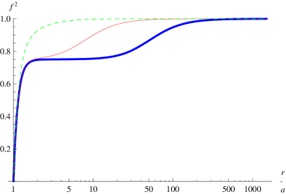
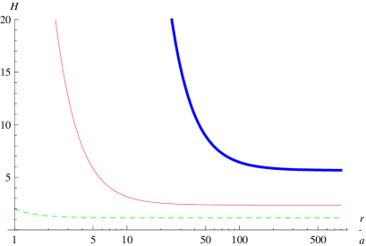
Figure 1: Numerical solution for $f^{2}(r)$ and $H(r)$, with the choice of parameters $k=10000$ and $a^{2}/\alpha^{\prime}k=\{0.0001,0.01,1\}$, respectively thick, thin and dashed lines.

In figure 1, we represent a family of such solutions with conformal factor having the asymptotics:

$$H(r)\stackrel{{\scriptstyle r\to a^{+}}}{{\sim}}1+\frac{\alpha^{\prime}k}{r^{2}}\,,\qquad\lim_{r\rightarrow\infty}H(r)=H_{\infty}\,,$$ (3.24)

and a function $f^{2}$ possessing a bolt singularity at $r=a$ (where the blow-up parameter $a$ has been set previously in defining the gauge bundle). The dilaton is then determined by the conformal factor, up to a constant, by integrating eq.(3.6a):

$$e^{2\Phi(r)}=e^{2\Phi_{0}}H(r)^{2}\,.$$ (3.25)

We observe in particular that since $\lim_{r\to\infty}f^{2}=1$, the solution interpolates between the squashed resolved conifold at finite $r$ and the usual cone over the Einstein space $T^{1,1}/\mathbb{Z}_{2}$ at infinity, thus restoring a Ricci-flat background asymptotically. In figure 1 we also note that in the regime where $a^{2}$ is small compared to $\alpha^{\prime}k$, the function $f^{2}$ develops a saddle point that disappears when their ratio tends to one.

As expected from this type of torsional backgrounds, in the blow-down limit the gauge bundle associated with $\vec{q}$ becomes a kind of point-like instanton, leading to a five-brane-like solution. The appearance of five-branes manifests itself by a singularity in the conformal factor $H$ in the $r\to 0$ limit, hence of the dilaton. In this limit the solution behaves as the backreaction of heterotic five-branes wrapping some supersymmetric vanishing two-cycle, together with a gauge bundle turned on. As we will see later on this singularity is not smoothed out by the $\mathcal{R}^{2}$ curvature correction to the Bianchi identity.

3.5 Analytical solution in the double-scaling limit

The regime $a^{2}/\alpha^{\prime}k\ll 1$ in parameter space allows for a limit where the system (3.6) admits an analytical solution, which corresponds to a sort of ’near-bolt’ or throat geometry of the family of torsional backgrounds seen above. This solution is valid in the coordinate range:

$$a^{2}\leqslant r^{2}\ll\alpha^{\prime}k\,.$$ (3.26)

Note that this is not a ’near-singularity’ regime as the location $a$ of the bolt is chosen hierarchically smaller than the scale $\sqrt{\alpha^{\prime}k}$ at which one enters the throat region.

This geometry can be extended to a full solution of heterotic supergravity by means of a double scaling limit, defined as

$$g_{s}\to 0\,,\qquad\qquad\mu=\frac{g_{s}\alpha^{\prime}}{a^{2}}\quad\text{fixed}\,,$$ (3.27)

and given in terms of the asymptotic string coupling $g_{s}=e^{\Phi_{0}}H_{\infty}$ set by the $r\to\infty$ limit of expression (3.25). This isolates the dynamics near the four-cycle of the resolved singularity, without going to the blow-down limit, i.e. keeping the transverse space to be conformal to the non-singular resolved conifold.

One obtains an interacting theory whose effective string coupling constant is set by the double-scaling parameter $\mu$. The metric is determined by solving (3.6) in this limit, yielding the analytic expressions:

$$H(r)=\frac{\alpha^{\prime}k}{r^{2}}\,,\qquad f^{2}(r)=g_{1}^{2}(r)=\tfrac{3}{4}\Big{[}1-\left(\frac{a}{r}\right)^{8}\Big{]}\,.$$ (3.28)

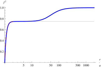
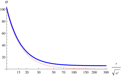
Figure 2: Comparison of the profiles of $f(r)$ and $H(r)$ for the asymptotically flat supergravity solution (thick line) and its double scaling limit (thin line), for $k=10000$ and $a^{2}/\alpha^{\prime}k=0.0001$.

To be more precise in defining the double-scaling limit one requests to stay at fixed distance from the bolt. We use then the rescaled dimensionless radial coordinate $R=r/a$, in terms of which one obtains the double scaling limit of the background (3.1,3.7,3.25):

$$\mathrm{d}s^{2} =\eta_{\mu\nu}\mathrm{d}x^{\mu}\mathrm{d}x^{\nu}+\frac{2\alpha^{\prime}k}{R^{2}}\,\biggl{[}\tfrac{\mathrm{d}R^{2}}{1-\tfrac{1}{R^{8}}}+\frac{R^{2}}{8}\,\Big{(}\mathrm{d}\theta_{2}^{2}+\sin^{2}\theta_{1}\,\mathrm{d}\phi_{1}^{2}+\mathrm{d}\theta_{2}^{2}+\sin^{2}\theta_{2}\,\mathrm{d}\phi_{2}^{2}\Big{)}$$

$$\hskip 128.0374pt+\,\frac{R^{2}}{16}(1-\tfrac{1}{R^{8}})\big{(}\mathrm{d}\psi+\cos\theta_{1}\,\mathrm{d}\phi_{1}+\cos\theta_{2}\,\mathrm{d}\phi_{2}\big{)}^{2}\biggr{]}\,,$$ (3.29a)

$$\mathcal{H}_{[3]} =\frac{\alpha^{\prime}k}{8}\,\Big{(}1-\tfrac{1}{R^{8}}\Big{)}\,\big{(}\Omega_{1}+\Omega_{2}\big{)}\wedge\tilde{\omega}\,,$$ (3.29b)

$$e^{\Phi(r)} =\frac{\mu}{H_{\infty}}\left(\frac{k}{R^{2}}\right)\,,$$ (3.29c)

$$\mathcal{A}_{[1]} =\tfrac{1}{4}\Big{[}\big{(}\cos\theta_{1}\,\mathrm{d}\phi_{1}-\cos\theta_{2}\,\mathrm{d}\phi_{2}\big{)}\,\vec{p}+\tfrac{1}{R^{4}}\,\tilde{\omega}\,\vec{q}\,\Big{]}\cdot\vec{H}\,,$$ (3.29d)

The warped geometry is a six-dimensional torsional analogue of Eguchi-Hanson space, as anticipated before in subsection 3.3. We observe that (as for the double-scaling limit of the warped Eguchi-Hanson space studied in [28]) the blow-up parameter $a$ disappears from the metric, being absorbed in the double-scaling parameter $\mu$, hence in the dilaton zero-mode that fixes the effective string coupling.

As can be read off from the asymptotic form of the metric (3.29), the metric of its $T^{1,1}$ base is non-Einstein even at infinity, so that the space is not asymptotically Ricci-flat, contrary to the full supergravity solution corresponding figure 1. But as expected, in the regime where $a^{2}\ll\alpha^{\prime}Q_{5}$ both the supergravity and the the near-horizon background agree perfectly in the vicinity of the bolt, as shown in figure 2.

Finally we notice that taking the near-brane limit of blown-down geometry (which amounts to replace $f^{2}$ by one in the metric (3.29a), and turning off the gauge bundle associated with $\vec{q}$) the six-dimensional metric factorizes into a linear dilaton direction and a non-Einstein $T^{1,1}/\mathbb{Z}_{2}$ space.

3.6 One-loop contribution to the Bianchi identity

The supergravity solution (3.1) is valid in the large charges regime $k\gg 1$, where higher derivative (one-loop) corrections to the Bianchi identity (2.3) are negligible. Given the general behaviour of the function $f^{2}$ and $H$ as plotted in figure 1, we must still verify that the curvature contribution $\text{tr}\,\mathcal{R}_{+}\wedge\mathcal{R}_{+}$ remains finite for large $k$ and arbitrary value of $a$, for any $r\geqslant a$, with coefficients of order one, so that the truncation performed on the Bianchi identity is consistent and the solution obtained is reliable.

We can give an ’on-shell’ expression of the one-loop contribution in (2.3) by using the supersymmetry equations (3.6) to re-express all first and second derivatives of $f$ and $H$ in terms of the functions $g_{1}$, $f$ and $H$ themselves. We obtain:

$$\begin{array}[]{l}{\displaystyle\mbox{tr}\,\mathcal{R}(\Omega_{+})\wedge\mathcal{R}(\Omega_{+})\,=}\\[6.0pt] {\displaystyle\qquad-4\Big{(}1-\frac{4f^{2}}{3}\big{(}2-f^{2}\big{)}-\frac{2g_{1}^{2}(1-f^{2})}{3}\Big{[}\frac{\alpha^{\prime}k}{r^{2}H}\Big{]}+\frac{2g_{1}^{4}}{3f^{2}}\Big{[}\frac{\alpha^{\prime}k}{r^{2}H}\Big{]}^{2}+\frac{2g_{1}^{6}}{9f^{2}}\Big{[}\frac{\alpha^{\prime}k}{r^{2}H}\Big{]}^{3}\Big{)}\,\Omega_{1}\wedge\Omega_{2}}\\[10.0pt] {\displaystyle\qquad\quad-8\Big{(}4(1-f^{2})^{2}+(1-f^{2})(1-4g_{1}^{2})\Big{[}\frac{\alpha^{\prime}k}{r^{2}H}\Big{]}+\frac{g_{1}^{2}\big{(}-6f^{2}+g_{1}^{2}(3+2f^{4}+6f^{2})}{3f^{4}}\Big{[}\frac{\alpha^{\prime}k}{r^{2}H}\Big{]}^{2}}\\[8.0pt] {\displaystyle\qquad\qquad+\frac{g_{1}^{4}\big{(}-3f^{2}+2g_{1}^{2}(1+2f^{2})\big{)}}{3f^{4}}\Big{[}\frac{\alpha^{\prime}k}{r^{2}H}\Big{]}^{3}+\frac{2g_{1}^{8}}{9f^{4}}\Big{[}\frac{\alpha^{\prime}k}{r^{2}H}\Big{]}^{4}\Big{)}\frac{\mathrm{d}r}{r}\wedge\big{(}\Omega_{1}+\Omega_{2}\big{)}\wedge\tilde{\omega}\,.}\end{array}$$ (3.30)

We observe from the numerical analysis of the previous subsection that $f\in[0,1]$ while $H$ is monotonously decreasing from $H_{\text{max}}=H(a)$ finite to $H_{\infty}>0$. So expression (3.30) remains finite at $r\rightarrow\infty$, since all overt $r$ contributions come in powers of $\alpha^{\prime}k/(r^{2}H)$, which vanishes at infinity.

Now, since $f$ and $g_{1}$ both vanish at $r=a$, there might also arise a potential divergences in (3.30) in the vicinity of the bolt. However:

• At $r=a$, all the potentially divergent terms appear as ratios: $g_{1}^{2n}\,f^{-2m}$, with $n\geq m$, and are thus zero or at most finite, since $g_{1}$ and $f$ are equal at the bolt.

• The other contributions all remain finite at the bolt, since they are all expressed as powers of $\alpha^{\prime}k/(r^{2}H)$, which is maximal at $r=a$, with:

  $$\text{Max}\Big{[}\frac{\alpha^{\prime}k}{r^{2}H}\Big{]}=\left(1+\frac{a^{2}}{\alpha^{\prime}k}\right)^{-1}\leq 1\,.$$

Taking the double-scaling limit, the expression (3.30) simplifies to:

$$\mbox{tr}\,\mathcal{R}(\Omega_{+})\wedge\mathcal{R}(\Omega_{+})=-\big{(}4-8g^{2}+5g^{4}\big{)}\,\Omega_{1}\wedge\Omega_{2}-2\big{(}16-34g^{2}+23g^{4}\big{)}\,\frac{\mathrm{d}r}{r}\wedge\big{(}\Omega_{1}+\Omega_{2}\big{)}\wedge\tilde{\omega}\,,$$ (3.31)

where $g_{1}$ has been rescaled to $g(r)=\sqrt{1-(a/r)^{8}}$ for simplicity. We see that this expression does not depend on $k$, because of the particular profile of $H$ in this limit (3.28), and is clearly finite of $\mathcal{O}(1)$ for $r\in[a,\infty[$.

Bianchi identity at the bolt

By using the explicit form for $\text{tr}\,\mathcal{R}_{+}\wedge\mathcal{R}_{+}$ determined above, we can evaluate the full Bianchi identity (2.3) at the bolt. At $r=a$, the nsns flux $\mathcal{H}$ vanishes, and the tree-level and one-loop contributions are both on the same footing. The Bianchi identity can be satisfied at the form level for (3.30):

$$0=\text{Tr}\,\mathcal{F}\wedge\mathcal{F}-\text{tr}\,\mathcal{R}(\Omega_{+})\wedge\mathcal{R}(\Omega_{+})=\big{(}\vec{p}^{\,2}-\vec{q}^{\,2}+4\big{)}\,\Omega_{1}\wedge\Omega_{2}\,$$ (3.32)

provided:

$$\vec{p}^{\,2}=\vec{q}^{\,2}-4\,.$$ (3.33)

As we will see in section 4.1 when deriving the worldsheet theory for the background (3.29), this result will be precisely reproduced in the cft by the worldsheet normally cancellation condition. It suggests that the $\alpha^{\prime}$ corrections to the supergravity solution vanish at the bolt, as the worldsheet result is exact.

Tadpole condition at infinity

In order to view the solution (3.1) as part of a compactification manifold, it is useful to consider the tadpole condition associated to it, as it has non-vanishing charges at infinity.

One requests at least to cancel the leading term in the asymptotic expansion of the modified Bianchi identity at infinity, where the metric becomes Ricci-flat, and the five-brane charge can thus in principle be set to zero (not however that the gauge bundle $V$ is different from the standard embedding). In this limit, only the first gauge bundle specified by the shift vector $\vec{p}$ contributes, so that (2.3) yields the constraint:

$$6Q_{5}=3\vec{p}^{\,2}-4\,.$$ (3.34)

Since $\vec{p}\in\mathbb{Z}^{16}$, we can never set the five-brane charge to zero and fulfil this condition. Furthermore, switching on the five-brane charge could only balance the instanton number of the gauge bundle, but never the curvature contribution, for elementary numerological reasons. Again, eq. (3.34) can only be satisfied in the large charge regime, where the one-loop contribution is subleading.

In the warped Eguchi-Hanson solution tackled in [28], the background was locally torsional but for some appropriate choice of Abelian line bundle the five-brane charge could consistently be set to zero; here no such thing occurs. This amounts to say that in the present case torsion is always present to counterbalance tree-level effects, while the only way to incorporate higher order contributions is to compute explicitly the one-loop correction to the background (3.1) from the Bianchi identity, as in [21]. In the double-scaling limit (3.29), this could in principle be carried out by the worldsheet techniques developed in [36, 37, 38], using the gauged wzw model description we discuss in the next section.

3.7 Torsion classes and effective superpotential

In this section we will delve deeper into the $SU(3)$ structure of the background as a way of characterizing the geometry and the flux background we are dealing with. We will briefly go through some elements of the classification of $SU(3)$-structure that we will need in the following (for a more detailled and general presentation, cf. [42, 44, 1]). On general grounds, as soon as it departs from Ricci-flatness, a given space acquires intrinsic torsion, which classifies the $G$-structure it is endowed with. According to its index structure, the intrinsic torsion $T^{i}_{\phantom{i}jk}$ takes value in $\Lambda^{1}\otimes\mathfrak{g}^{\perp}$, where $\Lambda^{1}$ is the space of one-forms, and $\mathfrak{g}\oplus\mathfrak{g}^{\perp}=\mathfrak{spin}(d)$, with $d$ the dimension of the manifold, and it therefore decomposes into irreducible $G$-modules $\mathcal{W}_{i}$.

Torsion classes of SU(3)-structure manifolds

The six-dimensional manifold of interest has $SU(3)$-structure, and can therefore be classified in terms of the following decomposition of $T$ into of irreducible representations of $SU(3)$:

$$\begin{array}[]{rcl}T\in\Lambda^{1}\otimes\mathfrak{su}(3)^{\perp}&=&\mathcal{W}_{1}\oplus\mathcal{W}_{2}\oplus\mathcal{W}_{3}\oplus\mathcal{W}_{4}\oplus\mathcal{W}_{5}\\[4.0pt] (\boldsymbol{3}+\bar{\boldsymbol{3}})\times(\boldsymbol{1}+\boldsymbol{3}+\bar{\boldsymbol{3}})&=&(\boldsymbol{1}+\boldsymbol{1})+(\boldsymbol{8}+\boldsymbol{8})+(\boldsymbol{6}+\bar{\boldsymbol{6}})+(\boldsymbol{3}+\bar{\boldsymbol{3}})+(\boldsymbol{3}+\bar{\boldsymbol{3}})\,.\end{array}$$ (3.35)

This induces a specific decomposition of the exterior derivatives of the $SU(3)$ structure $J$ and $\Omega$ onto the components of the intrinsic torsion $W_{i}\in\mathcal{W}_{i}$:

$$\mathrm{d}J =-\tfrac{3}{2}\,\text{Im}(W_{1}^{(1)}\,\bar{\Omega})+W_{4}^{(3+\bar{3})}\wedge J+W_{3}^{(6+\bar{6})}\,,$$ (3.36a)

$$\mathrm{d}\Omega =W_{1}^{(1)}\,J\wedge J+W_{2}^{(8)}\wedge J+W_{5}^{(\bar{3})}\wedge\Omega\,,$$ (3.36b)

which measures the departure from the Calabi-Yau condition $\mathrm{d}J=0$ and $\mathrm{d}\Omega=0$ ensuring Ricci-flatness.

We have in particular $W_{1}$ a complex $0$-form, $W_{2}$ a complex $(1,1)$-form and $W_{3}$ a real primitive $[(1,2)+(2,1)]$-form. $W_{4}$ is a real vector and $W_{5}^{(\bar{3})}$ is the anti-holomorphic part of the real one-form $W_{5}^{(3+\bar{3})}$, whose holomorphic piece is projected out in expression (3.36b). In addition $W_{2}$ and $W_{3}$ are primitives, i.e. they obey $J\lrcorner W_{i}=0$, with the generalized inner product of a $p$-form $\alpha_{[p]}$ and $q$-form $\beta_{[q]}$ for $p\leq q$ given by $\alpha\lrcorner\beta=\tfrac{1}{p!}\alpha_{m_{1}..m_{p}}\beta^{m_{1}..m_{p}}_{\phantom{m_{1}..m_{p}}m_{p+1}..m_{q}}$.

The torsion classes can be determined by exploiting the primitivity of $W_{2}$ and $W_{3}$ and the defining relations (2.7) of the $SU(3)$ structure. Thus, we can recover $W_{1}$ from both equations (3.36). In our conventions, we have then

$$W_{1}^{(1)}=\tfrac{1}{12}\,J^{2}\lrcorner\mathrm{d}\Omega\equiv\tfrac{1}{36}\,J^{3}\lrcorner(\mathrm{d}J\wedge\Omega)\,.$$ (3.37)

Likewise, one can compute $W_{4}$ and $W_{5}$, by using in addition the relations $J\lrcorner\Omega=J\lrcorner\bar{\Omega}=0$:

$$W_{4}^{(3+\bar{3})}=\frac{1}{2}\,J\lrcorner\mathrm{d}J\,,\qquad\bar{W}_{5}^{(3+\bar{3})}=-\tfrac{1}{8}\big{(}\bar{\Omega}\lrcorner\mathrm{d}\Omega+\bar{\Omega}\lrcorner\mathrm{d}\Omega\big{)}\,.$$ (3.38)

This in particular establishes $W_{4}$ as what is known as the Lee form of $J$, while, by rewriting $\bar{W}_{5}$ as $\bar{W}_{5}=-\tfrac{1}{2}\text{Re}\Omega\lrcorner\mathrm{d}\text{Re}\Omega=-\tfrac{1}{2}\text{Im}\Omega\lrcorner\mathrm{d}\text{Im}\Omega$, we observe that $W_{5}$ is the Lee form of $\text{Re}\Omega$ or $\text{Im}\Omega$, indiscriminately [44]. This alternative formulation in terms of the Lee form is characteristic of the classification of almost Hermitian manifolds.

The torsion class $W_{3}^{(6+\bar{6})}=W_{3}^{(6)}+W_{3}^{(\bar{6})}$ is a bit more involved to compute, but may be determined in components by contracting with the totally antisymmetric holomorphic and anti-holomorphic tensors of $SU(3)$, which projects to the $\boldsymbol{6}$ or $\bar{\boldsymbol{6}}$ of $SU(3)$:

$$(\star_{3}W_{3}^{(6)})_{\bar{a}\bar{b}}=\,(W_{3})^{\bar{c}\bar{d}}_{\phantom{cd}[\bar{a}}\,\bar{\Omega}_{\bar{b}]\bar{c}\bar{d}}\,,\qquad(\star_{\bar{3}}W_{3}^{(\bar{6})})_{ab}=(W_{3})^{cd}_{\phantom{cd}[a}\,\Omega_{b]cd}\,,$$ (3.39)

with the metric $\eta_{ab}=2\delta_{a}^{\phantom{a}\bar{b}}$ and the ”Hodge star products” in three dimensions given by $\star_{3}E^{\bar{a}\bar{b}}=\epsilon^{\bar{a}\bar{b}}_{\phantom{ab}c}\,E^{c}$, and $\star_{\bar{3}}(\bullet)$ applying to the complex conjugate of the former expression.

The nsns flux also decomposes into $SU(3)$ representations:

$$\mathcal{H}=-\tfrac{3}{2}\,\text{Im}(H^{(1)}\,\bar{\Omega})+H^{(3+\bar{3})}\wedge J+H^{(6+\bar{6})}\,.$$ (3.40)

As a general principle, since torsion is generated by flux, supersymmetry requires that the torsion classes (3.36) be supported by flux classes in the same representation of $SU(3)$. Thus, we observe in particular that there is no component of $\mathcal{H}$ in the $(\boldsymbol{8}+\boldsymbol{8})$, which implies that $W_{2}=0$, for our type of backgrounds.

The torsion classes of the warped resolved conifold

After this general introduction we hereafter give the torsion classes for the warped six-dimensional background (3.1) studied in this work. They can be extracted from the following differential conditions, which have been established using the supersymmetry equations (3.6) and the relation (3.21):

$$\mathrm{d}\Omega =2\mu(r)\,\big{(}e^{1256}+e^{1346}+i(e^{1356}-e^{1246})\big{)}\,,$$ (3.41a)

$$\mathrm{d}J =-\mu(r)\,\big{(}e^{123}+e^{145}\big{)}\,,$$ (3.41b)

$$\mathcal{H} =\mu(r)\,(e^{236}+e^{456})\,,$$ (3.41c)

with the function:

$$\mu(r)=\sqrt{\frac{2}{3}}\,\frac{2\alpha^{\prime}kg_{1}^{2}}{r^{3}H^{3/2}f}=-\sqrt{\frac{2}{3}}\frac{f}{\sqrt{H}}\,\Phi^{\prime}\,.$$ (3.42)

Since relations (3.41) imply satisfying the first supersymmetry condition (3.6a), this induces automatically $W_{1}=W_{2}=0$ (this can be checked explicitly in (3.41)), which in turn entails that the manifold (3.1a) is complex, since the complex structure is now integrable.

Then, using relations (3.38) and (3.39), one determines the remaining torsion classes:

$$W_{1}=W_{2}=W_{3}=0\,,$$ (3.43)

and

$$W_{4}^{(3+\bar{3})}=\tfrac{1}{2}\,W_{5}^{(3+\bar{3})}=-\mu(r)\,\text{Re}E^{3}\,.$$ (3.44)

They are supported by the flux:

$$H^{(3+\bar{3})}=-\mu(r)\,\text{Im}E^{3}\,.$$ (3.45)

Two remarks are in order. First, combining (3.36a) and (2.8b) leads to the generic relation $W_{4}=\mathrm{d}\Phi$, which is indeed satisfied by the Lee form (3.44) by taking into account expression (3.42). Secondly, the relation $W_{5}=2W_{4}$ in (3.44) is a particular case of the formula $W_{5}=(-1)^{n+1}2^{n-2}W_{4}$ [18, 44] which holds for a manifold with $SU(n)$ structure.

Effective superpotential

The effective superpotential of four-dimensional $\mathcal{N}=1$ supergravity for this particular solution, viewing the throat solution we consider as part of some heterotic flux compactification. It can be derived from a generalization of the Gukov-Vafa-Witten superpotential [56], which includes the full contribution from torsion and $\mathcal{H}$-flux [57], or alternatively using generalized calibration methods [58]. The general expression reads:

$$\mathcal{W}=\tfrac{1}{4}\int_{\mathcal{M}_{6}}\Omega\wedge(H+i\mathrm{d}J)\,.$$ (3.46)

We evaluate this expression on the solution (3.1) by using the results obtained in (3.43-3.45). This leads to the ’on-shell’ complexified Kähler structure

$$\mathcal{H}+i\,\mathrm{d}J=iW_{5}^{(\bar{3})}\wedge J=-i\mu(r)\,\bar{E}_{3}\wedge J\,,$$ (3.47)

which together with the first relation in (2.7) entails

$$\mathcal{W}=0$$ (3.48)

identically.

In Vafa’s setup of ref. [59], corresponding to D5-branes wrapping the two-cycle of the resolved conifold, this leads to an $\mathcal{N}=1$ Veneziano-Yankielowicz superpotential (where the resolution parameter is identified with the glueball superfield of the four dimensional super Yang-Mills theory), showing that the background is holographically dual to a confining theory, with a gaugino condensate. In our case having a vanishing superpotential means that the blow-up parameter $a$ corresponds to a modulus of the holographically dual $\mathcal{N}=1$ four-dimensional theory. More aspects of the holographic duality are discussed in subsection 6.1.

A Kähler potential for the non-Ricci-flat conifold

In the following, we will show that the manifold corresponding to the metric (3.1a) is conformally Kähler. This can be readily established by means of the differential conditions (3.36), as the characteristics of a given space are related to the vanishing of certain torsion classes or specific constraint relating them (see [1] for a general overlook).

For this purpose, we now have to determine the torsion classes for the resolved conifold space conformal to the geometry (3.1a):

$$\mathrm{d}s^{2}_{\tilde{\mathcal{C}}_{6}}=\frac{\mathrm{d}r^{2}}{f^{2}}+\frac{r^{2}}{6}\big{(}\mathrm{d}\Omega_{1}^{2}+\mathrm{d}\Omega_{2}^{2}\big{)}+\frac{r^{2}f^{2}}{9}\tilde{\omega}^{2}\,.$$ (3.49)

Again, these can be read from the differential conditions:

$$\mathrm{d}\tilde{\Omega} =\tfrac{3}{2}\,\tilde{\mu}(r)\,\big{(}\tilde{e}^{1256}+\tilde{e}^{1346}+i(\tilde{e}^{1356}-\tilde{e}^{1246})\big{)}\,$$ (3.50a)

$$\mathrm{d}\tilde{J} =0\,,$$ (3.50b)

with now

$$\tilde{\mu}(r)=\frac{\alpha^{\prime}k\left(1-\left(\frac{a}{r}\right)^{8}\right)}{r^{3}f(r)}\,.$$ (3.51)

and the new set of vielbeins given by:

$$\tilde{e}^{i}=\sqrt{\frac{2}{3H}}\,e^{i}\,,\qquad\forall i=1,..,6\,.$$ (3.52)

Repeating the analysis carried out earlier, the torsion classes are easily established:

$$W_{1}=W_{2}=W_{3}=W_{4}=0\,,$$ (3.53)

$$W_{5}^{(3+\bar{3})}=-2\tilde{\mu}(r)\,\text{Re}E^{3}\,,$$ (3.54)

The first relation (3.53) tells us that the manifold is complex, since $W_{1}=W_{2}=0$, and symplectic, since the Kähler form $\tilde{J}$ is closed. Fulfilling both these conditions gives precisely a Kähler manifold, and the Levi Civita connection is in this case endowed with $U(3)$ holonomy.

The Kähler potential

The Kähler potential for the conifold metric (3.49) is most easily computed by starting from the generic definition of the (singular) conifold as a quadratic on $\mathbb{C}^{4}$, whose base is determined by the intersection of this quadratic with a three-sphere of radius $\varrho$. These two conditions are summarized in [31]:

$$\mathcal{C}_{6}\stackrel{{\scriptstyle\mbox{def}}}{{=}}\sum_{A=1}^{4}(w_{A})^{2}=0\,\qquad\sum_{A=1}^{4}|w_{A}|^{2}=\varrho^{2}\,.$$ (3.55)

One can rephrase these two conditions in terms of a $2\times 2$ matrix $W$ parametrizing the $T^{1,1}$ base of the conifold, viewed as the coset $(SU(2)\times SU(2))/U(1)$, as $W=\tfrac{1}{\sqrt{2}}\sum_{A}w^{A}\sigma_{A}$. In this language, the defining equations (3.55) take the form:

$$\text{det}\,W=0\,,\qquad\text{tr}\,W^{\dagger}W=\varrho^{2}\,.$$ (3.56)

For the Kähler potential $\mathcal{K}$ to generate the metric (3.49), it has to be invariant under the action of the rotation group $SO(4)\simeq SU(2)\times SU(2)$ of (3.55) and can thus only depend on $\varrho^{2}$. In terms of $\mathcal{K}$ and $W$, the metric on the conifold reads:

$$\mathrm{d}s^{2}=\dot{\mathcal{K}}\,\text{tr}\,\mathrm{d}W^{\dagger}\mathrm{d}W+\ddot{\mathcal{K}}\,|\text{tr}\,W^{\dagger}\mathrm{d}W|^{2}\,,$$ (3.57)

where the derivative is $\dot{(\bullet)}\equiv\frac{\partial}{\partial\rho^{2}}(\bullet)$. By defining the function $\gamma(\varrho)=\varrho^{2}\,\dot{\mathcal{K}}$, the metric (3.57) can be recast into the form:

$$\mathrm{d}s^{2}=\dot{\gamma}\,\mathrm{d}\varrho^{2}+\frac{\gamma}{4}\big{(}\mathrm{d}\Omega_{1}^{2}+\mathrm{d}\Omega_{2}^{2}\big{)}+\frac{\varrho^{2}\dot{\gamma}}{4}\,\tilde{\omega}^{2}\,.$$ (3.58)

Identifying this expression with the metric (3.49) yields two independent first order differential equations, one of them giving the expression of the radius of the $S^{3}$ in (3.55) in terms of the radial coordinate in (3.49):

$$\varrho=\varrho_{0}\,e^{{\displaystyle\tfrac{3}{2}\int\frac{\mathrm{d}r}{rf^{2}}}}\,,\qquad\gamma(r)=\tfrac{2}{3}\,r^{2}\,.$$ (3.59)

From these relations, one derives the Kähler potential as a function of $r$:

$$\mathcal{K}(r)=\mathcal{K}_{0}+\int\frac{\mathrm{d}(r^{2})}{f^{2}}\,.$$ (3.60)

In particular, we can work out $\mathcal{K}$ explicitly in the near horizon limit (3.27):

$$\mathcal{K}(r)=\mathcal{K}_{0}+\frac{4a^{2}}{3}\,\left[\left(\frac{r}{a}\right)^{2}-\frac{1}{2}\text{arctan}\left(\frac{r}{a}\right)^{2}+\frac{1}{4}\log\left(\frac{r^{2}-a^{2}}{r^{2}+a^{2}}\right)\right]\,.$$ (3.61)

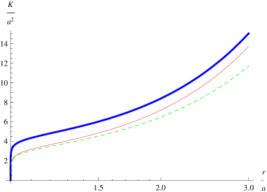
Figure 3: The Kähler potential for the asymptotically flat supergravity solution with $k=10000$ and $a^{2}/\alpha^{\prime}k=\{0.0001,0.01,1\}$.

Choosing $\varrho_{0}=1$, we have $\varrho=\sqrt[4]{r^{8}-a^{8}}$, which varies over $[0,\infty[$, as expected. With an exact Kähler potential at our disposal, we can make an independent check that the near horizon geometry (3.29) is never conformally Ricci flat. Indeed, by establishing the Ricci tensor $R_{i\bar{\jmath}}=\partial_{i}\partial_{\bar{\jmath}}\ln\sqrt{|g|}$ for the Kähler manifold (3.57), we observe that the condition for Ricci flatness imposes the relation $\partial_{\varrho^{2}}[(\varrho^{2}\dot{\mathcal{K}})^{3}]=2\varrho^{2}$ [32], which is never satisfied by the potential (3.61).

In figure 3 we plot the Kähler potential (3.60) for the asymptotically Ricci-flat supergravity backgrounds given in figure 1. We represent $\mathcal{K}$ only for small values of $r$, since for large $r$ it universally behaves like $r^{2}$. One also verifies that, for small $r$, the analytic expression (3.61) determined in the double-scaling limit fits perfectly the numerical result.

4 Gauged WZW model for the Warped Resolved Orbifoldized Conifold

The heterotic supergravity background obtained in the first section has been shown to admit a double scaling limit, isolating the throat region where an analytical solution can be found. The manifold is conformal to a cone over a non-Einstein $T^{1,1}/\mathbb{Z}_{2}$ base with a blown-up four-cycle, and features an asymptotically linear dilaton. The solution is parametrized by two ’shift vectors’ $\vec{p}$ and $\vec{q}$ which determine the Abelian gauge bundle, and are orthogonal to each other. They are related to the nsns flux number $k$ as $k=\vec{p}^{\,2}=\vec{q}^{\,2}$. These conditions, as well as the whole solution (3.29), are valid in the large charge limit $\vec{p}^{\,2}\gg 1$.

The presence of an asymptotic linear dilaton is a hint that an exact worldsheet cft description may exist. We will show in this section that it is indeed the case; for any consistent choice of line bundle, a gauged wzw model, whose background fields are the same as the supergravity solution (3.29), exists. Before dealing with the details let us stress important points of the worldsheet construction:

1. In the blow-down limit $a\to 0$, the dependence of the metric on the radial coordinate simplifies, factorizing the space into the (non-Einstein) $T^{1,1}$ base times the linear dilaton direction $r$.

2. The $T^{1,1}$ space is obtained as an asymmetrically gauged $SU(2)_{k}\times SU(2)_{k}$ wzw-model involving the right-moving current algebra of the heterotic string.

3. In order to find the blown-up solution the linear dilaton needs to be replaced by an auxiliary $SL(2,\mathbb{R})_{k/2}$ wzw-model. It is gauged together with the $SU(2)\times SU(2)$ factor, also in an asymmetric way.

4. The ’shift vectors’ $\vec{p}$ and $\vec{q}$ define the embedding of the both gaugings in the $Spin(32)/\mathbb{Z}_{2}$ lattice

5. These two worldsheet gaugings are anomaly-free if $k=\vec{p}^{\,2}=\vec{q}^{\,2}-4$ and $\vec{p}\cdot\vec{q}=0$. These relations are exact in $\alpha^{\prime}$.

A detailed study of a related model, based on a warped Eguchi-Hanson space, is given in ref. [28]. We refer the reader to this work for more details on the techniques used hereafter.

4.1 Parameters of the gauging

We consider an $\mathcal{N}=(1,0)$ wzw model for the group $SU(2)\times SU(2)\times SL(2,\mathbb{R})$, whose element we denote by $(g_{1},g_{2},h)$. The associated levels of the $\mathcal{N}=1$ affine simple algebras are respectively chosen to be $k$, $k$ and $k^{\prime}$. The left-moving central charge reads

$$c=9-\frac{12}{k}+\frac{6}{k^{\prime}}\,,$$ (4.1)

therefore the choice $k^{\prime}=k/2$ ensures that the central charge has the requested value $c=9$ for any $k$, allowing to take a small curvature supergravity limit $k\to\infty$.

The first gauging, yielding a $T^{1,1}$ coset space with a non-Einstein metric, acts on $SU(2)\times SU(2)$ as

$$\Big{(}g_{1}(z,\bar{z}),g_{2}(z,\bar{z})\Big{)}\longrightarrow\Big{(}e^{i\sigma_{3}\alpha(z,\bar{z})}g_{1}(z,\bar{z}),e^{-i\sigma_{3}\alpha(z,\bar{z})}g_{2}(z,\bar{z})\Big{)}\,.$$ (4.2)

This gauging is highly asymmetric, acting only by left multiplication. It has to preserve $\mathcal{N}=(1,0)$ superconformal symmetry on the worldsheet, hence the worldsheet gauge fields are minimally coupled to the left-moving worldsheet fermions of the super-wzw model.

In addition, the classical anomaly from this gauging can be cancelled by minimally coupling some of the 32 right-moving worldsheet fermions of the heterotic worldsheet theory. We introduce a sixteen-dimensional vector $\vec{p}$ that gives the embedding of the gauging in the $\mathfrak{so}(32)$ Cartan sub-algebra. The anomaly cancellation condition gives the constraint

$$k+k=2\vec{p}^{\,2}\implies k=\vec{p}^{\,2}\,.$$ (4.3)

On the left-hand side, the two factors correspond to the gauging in both $SU(2)_{k}$ models. We denote the components of the worldsheet gauge field as $(A,\bar{A})$.

The second gauging, leading to the resolved conifold, also acts on the $SL(2,\mathbb{R})_{k^{\prime}}$ factor, along the elliptic Cartan sub-algebra (which is time-like). Its action is given as follows:

$$\Big{(}g_{1}(z,\bar{z}),g_{2}(z,\bar{z}),h(z,\bar{z})\Big{)}\\ \longrightarrow\ \Big{(}e^{i\sigma_{3}\beta_{1}(z,\bar{z})}g_{1}(z,\bar{z}),e^{i\sigma_{3}\beta_{1}(z,\bar{z})}g_{2}(z,\bar{z}),e^{2i\sigma_{3}\beta_{1}(z,\bar{z})}h(z,\bar{z})e^{2i\sigma_{3}\,\beta_{2}(z,\bar{z})}\Big{)}\,,$$ (4.4)

and requires a pair of worldsheet gauge fields $\mathbf{B}=(B_{1},B_{2})$. The left gauging, corresponding to the gauge field $B_{1}$, is anomaly-free (without the need of right-moving fermions) for

$$2k=4k^{\prime}\,,$$ (4.5)

which is satisfied by the choice $k^{\prime}=k/2$ that was assumed above. The other gauging, corresponding to the gauge field $B_{2}$, acts only on $SL(2,\mathbb{R})$, by right multiplication. This time the coupling to the worldsheet gauge field need not be supersymmetric, as we are dealing with a $\mathcal{N}=(1,0)$ (heterotic) worldsheet.

The anomaly is again cancelled by minimally coupling worldsheet fermions from the gauge sector. Denoting the corresponding shift vector $\vec{q}$ one gets the condition

$$4\left(\frac{k}{2}+2\right)=2\vec{q}^{\,2}\implies k=\vec{q}^{\,2}-4\,,$$ (4.6)

which involves the bosonic level of $SL(2,\mathbb{R})$, as explained above; the constant term on the rhs corresponds to the renormalization of the background fields by $\alpha^{\prime}$ corrections, exact to all orders. In order to avoid the appearance of mixed anomalies in the full gauged wzw model, one chooses the vectors defining the two gaugings to be orthogonal to each other

$$\vec{p}\cdot\vec{q}=0\,.$$ (4.7)

4.2 Worldsheet action for the gauged WZW model

The total action for the gauged wzw model defined above is given as follows:

$$S_{\textsc{wzw}}(A,{\bf B})=S_{SL(2,\mathbb{R})_{k/2+2}}+S_{SU(2)_{k-2},\,1}+S_{SU(2)_{k-2},\,2}+S_{\text{gauge}}(A,{\bf B})+S_{\text{Fer}}(A,{\bf B})\,,$$ (4.8)

where the first three factors correspond to bosonic wzw actions, the fourth one to the bosonic terms involving the gauge fields and the last one to the action of the minimally coupled fermions. As it proves quite involved, technically speaking, to tackle the general case for generic values of the shift vectors $\vec{p}$ and $\vec{q}$, we restrict, for simplicity, to the ’minimal’ solution of the constraints (4.6,4.7) given by

$$\vec{p}=(2\ell,0^{15})\ ,\quad\vec{q}=(0,2\ell,2,0^{13})\qquad\text{with}\quad\ell>2\,,$$ (4.9)

implying in particular $k=4\ell^{2}$. This choice ensures that $k$ is even, which will later on show to be necessary when considering the orbifold. The coset theory constructed with these shift vectors involves overall six Majorana-Weyl right-moving fermions from the sixteen participating in the fermionic representation of the $Spin(32)/\mathbb{Z}_{2}$ lattice.

We parametrize the group-valued worldsheet scalars $(g_{1},g_{2},h)\in SU(2)\times SU(2)\times SL(2,\mathbb{R})$ in terms of Euler angles as follows:

$$g_{\ell} =e^{\frac{i}{2}\sigma_{3}\psi_{\ell}}e^{\frac{1}{2}\sigma_{1}\theta_{\ell}}e^{\frac{i}{2}\sigma_{3}\phi_{\ell}}\ ,\quad\ell=1,2$$ (4.10a)

$$h =e^{\frac{i}{2}\sigma_{3}\phi_{L}}e^{\frac{1}{2}\sigma_{1}\rho}e^{\frac{i}{2}\sigma_{3}\phi_{R}}\,,\quad$$ (4.10b)

where $\sigma_{i}$, $i=1,..,3$, are the usual Pauli matrices.

The action for the worldsheet gauge fields, including the couplings to the bosonic affine currents of the wzw models, is given by:

$$S_{\text{gauge}}(A,{\bf B})=\frac{1}{8\pi}\int\mathrm{d}^{2}z\,\Big{[}2i\big{(}j^{3}_{1}-j^{3}_{2}\big{)}\bar{A}\,+\,2(k-2)A\bar{A}\,+\,2B_{1}i\bar{k}^{3}+2i\big{(}j^{3}_{1}+j^{3}_{2}+2k^{3}\big{)}\bar{B}_{2}\\ +\,2(k-2)B_{2}\bar{B}_{2}\,-\,\left(\tfrac{k}{2}+2\right)\big{(}B_{1}\bar{B}_{1}+4B_{2}\bar{B}_{2}+4\cosh\rho\,B_{1}\bar{B}_{2}\big{)}\Big{]}\,.$$ (4.11)

The action for the worldsheet fermions comprises the left-moving Majorana-Weyl fermions coming from the $SU(2)\times SU(2)\times SL(2,\mathbb{R})$ $\mathcal{N}=(1,0)$ super-wzw action, respectively ($\zeta^{1},\zeta^{2})$, ($\zeta^{3},\zeta^{4})$ and ($\zeta^{5},\zeta^{6})$, supplemented by six right-moving Majorana-Weyl fermions coming from the $Spin(32)_{1}/\mathbb{Z}_{2}$ sector, that we denote $\bar{\xi}^{a}$, $a=1,..,6$:

$$S_{\text{Fer}}(A,{\bf B})=\frac{1}{4\pi}\int\mathrm{d}^{2}z\,\Big{[}\sum_{i=1}^{6}\zeta^{i}\bar{\partial}\zeta^{i}-2\big{(}\zeta^{1}\zeta^{2}-\zeta^{3}\zeta^{4}\big{)}\bar{A}\\ -2\big{(}\zeta^{1}\zeta^{2}+\zeta^{3}\zeta^{4}+2\zeta^{5}\zeta^{6}\big{)}\bar{B}_{2}+\sum_{a=1}^{6}\bar{\xi}^{a}\partial\bar{\xi}^{a}-2\ell A\,\bar{\xi}^{1}\bar{\xi}^{2}-2\bar{B}_{1}\big{(}\bar{\xi}^{3}\bar{\xi}^{4}+\ell\bar{\xi}^{5}\bar{\xi}^{6}\big{)}\Big{]}\,.$$ (4.12)

Note in particular that both actions (4.11) and (4.12) are in keep with the normalization of the gauge fields required by the peculiar form of the second (asymmetric) gauging (4.4).

4.3 Background fields at lowest order in $\alpha^{\prime}$

Finding the background fields corresponding to a heterotic coset theory is in general more tricky than for the usual bosonic or type ii cosets, because of the worldsheet anomalies generated by the various pieces of the asymmetrically gauged wzw model. In our analysis, we will closely follow the methods used in [62, 38]. A convenient way of computing the metric, Kalb-Ramond and gauge field background from a heterotic gauged wzw model consists in bosonizing the fermions before integrating out the gauge field.

One will eventually need to refermionize the appropriate scalars to recover a heterotic sigma-model in the standard form, i.e. (see [63, 64]):

$$S=\frac{1}{4\pi}\int\!\!\mathrm{d}^{2}z\,\Big{[}\tfrac{2}{\alpha^{\prime}}(g_{ij}+\mathcal{B}_{ij})\partial X^{i}\bar{\partial}X^{j}+g_{ij}\zeta^{i}\bar{\nabla}(\Omega_{+})\zeta^{j}+\bar{\xi}^{A}\nabla(\mathcal{A})_{AB}\bar{\xi}^{B}+\tfrac{1}{4}\mathcal{F}^{AB}_{ij}\bar{\xi}_{A}\bar{\xi}_{B}\zeta^{i}\zeta^{j}\Big{]}$$ (4.13)

where the worldsheet derivative $\bar{\nabla}(\Omega_{+})$ is defined with respect to the spin connexion $\Omega_{+}$ with torsion and the derivative $\nabla(\mathcal{A})$ with respect to the space-time gauge connexion $\mathcal{A}$.

The details of this bosonization-refermionization procedure for the coset under scrutiny are given in appendix A. At leading order in $\alpha^{\prime}$ (or more precisely at leading order in a $1/k$ expansion) we thus obtain, after integrating out classically the gauge fields, the bosonic part of the total action as follows:

$$S_{\textsc{b}}=\frac{k}{8\pi}\int\mathrm{d}^{2}z\,\left[\frac{1}{2}\partial\rho\bar{\partial}\rho+\partial\theta_{1}\bar{\partial}\theta_{1}+\partial\theta_{2}\bar{\partial}\theta_{2}+\sin^{2}\theta_{1}\,\partial\phi_{1}\bar{\partial}\phi_{1}+\sin^{2}\theta_{2}\,\partial\phi_{2}\bar{\partial}\phi_{2}\right.\\ +\tfrac{1}{2}\tanh^{2}\rho\,(\partial\psi+\cos\theta_{1}\,\partial\phi_{1}+\cos\theta_{2}\,\partial\phi_{2})(\bar{\partial}\psi+\cos\theta_{1}\,\bar{\partial}\phi_{1}+\cos\theta_{2}\,\bar{\partial}\phi_{2})\\ \left.+\frac{1}{2}\big{(}\cos\theta_{1}\,\partial\phi_{1}+\cos\theta_{2}\,\partial\phi_{2}\big{)}\bar{\partial}\psi-\frac{1}{2}\partial\psi\big{(}\cos\theta_{1}\,\bar{\partial}\phi_{1}+\cos\theta_{2}\,\bar{\partial}\phi_{2}\big{)}\right]\,,$$ (4.14)

while the fermionic part of the action is given by

$$S_{\textsc{f}}=\frac{k}{4\pi}\int\mathrm{d}^{2}z\,\Big{[}\sum_{i=1}^{6}\zeta^{i}\bar{\partial}\zeta^{i}+(\bar{\zeta}^{1},\bar{\zeta}^{2})\big{[}{\rm 1\kern-2.79999ptI}_{2}\,\partial+(\cos\theta_{1}\,\partial\phi_{1}-\cos\theta_{2}\,\partial\phi_{2})\,i\sigma^{2}\big{]}\left(\begin{matrix}\bar{\xi}^{1}\\ \bar{\xi}^{2}\end{matrix}\right)\\ +\bar{\Xi}^{\top}\left[{\rm 1\kern-2.79999ptI}_{4}\,\partial+\frac{\ell}{\cosh\rho}\big{(}\partial\psi+\cos\theta_{1}\,\partial\phi_{1}+\cos\theta_{2}\,\partial\phi_{2}\big{)}\,i\sigma^{2}\otimes\left(\begin{matrix}1&0\\ 0&\ell\end{matrix}\right)\right]\bar{\Xi}\\ -\tfrac{1}{\ell}\,\bar{\xi}^{1}\bar{\xi}^{2}\,\big{(}\zeta^{1}\zeta^{2}-\zeta^{3}\zeta^{4}\big{)}+\frac{1}{\ell^{2}\cosh\rho}\,\big{(}\bar{\xi}^{3}\bar{\xi}^{4}+\ell\bar{\xi}^{5}\bar{\xi}^{6}\big{)}\big{(}\zeta^{1}\zeta^{2}+\zeta^{3}\zeta^{4}+2\zeta^{5}\zeta^{6}\big{)}\Big{]}\,,$$ (4.15)

with $\bar{\Xi}^{\top}=(\bar{\xi}^{3},\bar{\xi}^{4},\bar{\xi}^{5},\bar{\xi}^{6})$. In addition, a non-trivial dilaton is produced by the integration of the worldsheet gauge fields

$$\Phi=\Phi_{0}-\tfrac{1}{2}\ln\cosh\rho\,.$$ (4.16)

The background fields obtained above exactly correspond to the double-scaling limit of the supergravity solution (3.29) for a particular choice of vectors $\vec{p}$ and $\vec{q}$, after the change of coordinate

$$\cosh\rho=(r/a)^{4}=R^{4}\,.$$ (4.17)

As noticed in section 3.5, the blow-up parameter, which is not part of the definition of the coset cft, is absorbed in the dilaton zero-mode. It is straightforward – but cumbersome – to extend the computation to a more generic choice of bundle. This would lead to the background fields reproducing the generic supergravity solution (3.29).

In this section we left aside the discussion of the necessary presence of a $\mathbb{Z}_{2}$ orbifold acting on the $T^{1,1}$ base of the conifold. Its important consequences will be tackled below.

5 Worldsheet Conformal Field Theory Analysis

In this section we provide the algebraic construction of the worldsheet cft corresponding to the $\mathcal{N}=(1,0)$ gauged wzw model defined in section 4. We have shown previously that the non-linear sigma model with the warped deformed orbifoldized conifold as target space is given by the asymmetric coset:

$$\frac{SL(2,\mathbb{R})_{k/2}\times\,\left(\text{\small\raisebox{-2.84526pt}{$U(1)_{\textsc{l}}$}\! $\backslash$ \!\!\raisebox{2.84526pt}{$SU(2)_{k}\times SU(2)_{k}$}}\right)}{U(1)_{\textsc{l}}\times U(1)_{\textsc{r}}}\,,$$ (5.1)

which combines a left gauging of $SU(2)\times SU(2)$ with a pair of chiral gaugings which also involve the $SL(2,\mathbb{R})$ wzw model. In addition, the full worldsheet cft comprises a flat $\mathbb{R}^{3,1}$ piece, the right-moving heterotic affine algebra and an $\mathcal{N}=(1,0)$ superghost system. We will see later on that the coset (5.1) has an enhanced worldsheet $\mathcal{N}=(2,0)$ superconformal symmetry, which allows to achieve $\mathcal{N}=1$ target-space supersymmetry.

In the following, we will segment our algebraic analysis of the worldsheet cft for clarity’s sake, and deal separately with the singular conifold case, before moving on to treat the resolved geometry. This was somehow prompted by fact that the singular construction appears as a non-trivial building block of the ’resolved’ cft, as we shall see below.

5.1 A cft for the $T^{1,1}$ coset space

For this purpose, we begin by restricting our discussion to the cft underlying the non-Einstein $T^{1,1}$ base of the conifold, which is captured by the coset space $[SU(2)\times SU(2)]/U(1)$. In addition, this space supports a gauge bundle specified by the vector of magnetic charges $\vec{p}$. Then, the full quantum theory describing the throat region of heterotic strings on the torsional singular conifold, can be constructed by tensoring this cft with $\mathbb{R}^{3,1}$, the heterotic current algebra and a linear dilaton $\mathbb{R}_{\mathcal{Q}}$ with background charge

$$\mathcal{Q}=\sqrt{\frac{4}{k}}\,.$$ (5.2)

Focusing now on the $T^{1,1}$ space, we recall the action (4.2) of the first gauging on the group element $(g_{1},g_{2})\in SU(2)\times SU(2)$, supplemented with an action on the left-moving fermions dictated by $\mathcal{N}=1$ worldsheet supersymmetry. As seen in section 4, the anomaly following from this gauging is compensated by a minimal coupling to the worldsheet fermions of the gauge sector of the heterotic string, specified by the shift vector $\vec{p}$.

By algebraically solving the coset cft associated with this gauged wzw model, we are led to the following constraints on the zero-modes of the affine currents $J^{3}_{1.2}$ of the $SU(2)\times SU(2)$ Cartan subalgebra:

$$(J^{3}_{1})_{0}-(J^{3}_{2})_{0}=\vec{p}\cdot\vec{Q}_{\textsc{f}}\,,$$ (5.3)

where $\vec{Q}_{\textsc{f}}$ denotes the $\mathfrak{so}(32)$ weight of a given state. The affine currents of the $\widehat{\mathfrak{so}(32)}$ algebra can be alternatively written in the fermionic or bosonic representation as

$$\bar{\jmath}^{i}(\bar{z})=\bar{\xi}^{2i-1}\bar{\xi}^{2i}(\bar{z})=\sqrt{\frac{2}{\alpha^{\prime}}}\,\bar{\partial}X^{i}(\bar{z})\quad,\qquad i=1,\ldots 16\,,$$ (5.4)

and the components of $\vec{Q}_{\textsc{f}}$ can be identified with the corresponding fermion number (mod 2).

In order to explicitly solve the zero-mode constraint (5.3) at the level of the one-loop partition function, it is first convenient to split the left-moving supersymmetric $SU(2)$ characters in terms of the characters of an $SU(2)/U(1)$ super-coset:

$$\chi^{j}\vartheta{a\atopwithdelims[ ]b}=\sum_{m\in\mathbb{Z}_{2k}}C^{j}_{m}{a\atopwithdelims[ ]b}\Theta_{m,k}\,.$$ (5.5)

Next, to isolate the linear combination of Cartan generators appearing in (5.3), one can combine the two theta-functions at level $k$ corresponding to the Cartan generators of the two $\widehat{\mathfrak{su}(2)}_{k}$ algebras by using the product formula:

$$\Theta_{m_{1},k}\Theta_{m_{2},k}=\sum_{s\in\mathbb{Z}_{2}}\Theta_{m_{1}-m_{2}+2ks,2k}\Theta_{m_{1}+m_{2}+2ks,2k}\,.$$ (5.6)

Thus, the gauging yielding the $T^{1,1}$ base will effectively ’remove’ the $U(1)$ corresponding to the first theta-function. For simplicity, we again limit ourselves to the same minimal choice of shift vectors as in (4.9), namely $\vec{p}=(2\ell,0^{15})$, $\ell\in\mathbb{Z}$, which implies by (4.3)

$$k=4\ell^{2}\,.$$ (5.7)

Then the gauging will involve only a single right-moving Weyl fermion. Its contribution to the partition function is given by a standard fermionic theta-function:

$$\vartheta{u\atopwithdelims[ ]v}(\tau)=\sum_{N\in\mathbb{Z}}q^{\frac{1}{2}(N+\frac{u}{2})^{2}}e^{i\pi v(N+\frac{u}{2})}\,,$$ (5.8)

where ${u\atopwithdelims[ ]v}$ denote the spin structure on the torus. The solutions of the zero-mode constraint (5.3) can be obtained from the expressions (5.6) and (5.8). It gives (see [65, 66] for simpler cosets of the same type):

$$m_{1}-m_{2}=2\ell(2M+u)\quad,\qquad M\in\mathbb{Z}_{2\ell}\,.$$ (5.9)

We are then left, for given $SU(2)$ spins $j_{1}$ and $j_{2}$, with contributions to the coset partition function of the form

$$\sum_{m_{1}\in\mathbb{Z}_{8\ell^{2}}}C^{j_{1}}_{m_{1}}{a\atopwithdelims[ ]b}\,\bar{\chi}^{j_{1}}\,\sum_{M\in\mathbb{Z}_{2\ell}}e^{i\pi v(M+\tfrac{u}{2})}C^{j_{2}}_{m_{1}-2\ell(2M+u)}{a\atopwithdelims[ ]b}\,\bar{\chi}^{j_{2}}\,\sum_{s\in\mathbb{Z}_{2}}\Theta_{2m_{1}-2\ell(2M+u)+8\ell^{2}s,8\ell^{2}}\,.$$ (5.10)

One can in addition simplify this expression using the identity

$$\sum_{s\in\mathbb{Z}_{2}}\Theta_{2m_{1}-2\ell(2M+u)+8\ell^{2}s,8\ell^{2}}=\Theta_{m_{1}-\ell(2M+u),2\ell^{2}}\,.$$ (5.11)

Note that the coset partition function by itself cannot be modular invariant, since fermions from the gauge sector of the heterotic string were used in the coset construction.

5.2 Heterotic strings on the singular conifold

The full modular-invariant partition function for the singular torsional conifold case can now be established by adding (in the light-cone gauge) the $\mathbb{R}^{2}\times\mathbb{R}_{\mathcal{Q}}$ contribution, together with the remaining gauge fermions. Using the coset defined above, one then obtains the following one-loop amplitude:

$$Z(\tau,\bar{\tau})=\frac{1}{(4\pi\tau_{2}\alpha^{\prime})^{5/2}}\frac{1}{\eta^{3}\bar{\eta}^{3}}\,\frac{1}{2}\sum_{a,b}(-)^{a+b}\frac{\vartheta{a\atopwithdelims[ ]b}^{2}}{\eta^{2}}\sum_{m_{1}\in\mathbb{Z}_{2k}}\sum_{M\in\mathbb{Z}_{2\ell}}\,\frac{1}{2}\sum_{u,v\in\mathbb{Z}_{2}}\frac{\Theta_{m_{1}-2\ell(M+u/2),2\ell^{2}}}{\eta}\,\times\\[4.0pt] \times\,\sum_{2j_{1},2j_{2}=0}^{k-2}C^{j_{1}}_{m_{1}}{a\atopwithdelims[ ]b}C^{j_{2}}_{m_{1}-2\ell(2M+u)}{a\atopwithdelims[ ]b}e^{i\pi v(M+\tfrac{u}{2})}\bar{\chi}^{j_{1}}\bar{\chi}^{j_{2}}\,\frac{\bar{\vartheta}{u\atopwithdelims[ ]v}^{15}}{\bar{\eta}^{15}}\,.$$ (5.12)

The terms on the second line correspond to the contribution of the $\mathbb{R}^{2}\times\mathbb{R}_{\mathcal{Q}}\times U(1)$ piece with the associated left-moving worldsheet fermions. Their spin structure is given by ${a\atopwithdelims[ ]b}$, with $a=0$ (resp. $a=1$) corresponding to the ns (resp. r) sector. Again, the spin structure of the right-moving heterotic fermions for the $Spin(32)/\mathbb{Z}_{2}$ lattice is denoted by ${u\atopwithdelims[ ]v}$ (see the last term in this partition function). One may as well consider the $E_{8}\times E_{8}$ heterotic string theory, by changing the spin structure accordingly.

We notice that the full right-moving $SU(2)\times SU(2)$ affine symmetry, corresponding to the isometries of the $S^{2}\times S^{2}$ part of the geometry, is preserved, while the surviving left-moving $U(1)$ current represents translations along the $S^{1}$ fiber. In the partition function (5.12), the $U(1)$ charges are given by the argument of the theta-function at level $2\ell^{2}$. Later on, we will realize this $U(1)$ in terms of the canonically normalized free chiral boson $X_{\textsc{l}}(z)$.

Space-time supersymmetry

The left-moving part of the cft constructed above, omitting the flat space piece, can be described as an orbifold of the superconformal theories:

$$\left[\mathbb{R}_{1/\ell}\times U(1)_{2\ell^{2}}\right]\times\frac{SU(2)_{k}}{U(1)}\times\frac{SU(2)_{k}}{U(1)}\,.$$ (5.13)

The term between the brackets corresponds to a linear dilaton $\rho$ with background charge $\mathcal{Q}=\tfrac{1}{\ell}$, together with a $U(1)$ at level $2\ell^{2}$ (associated with the bosonic field $X_{\textsc{l}}$) and a Weyl fermion. This system has $\mathcal{N}=(2,0)$ supersymmetry, as it can be viewed as the holomorphic part of $\mathcal{N}=2$ Liouville theory at zero coupling. The last two factors are $SU(2)/U(1)$ super-cosets which are $\mathcal{N}=2$ minimal models. One then concludes that the left-moving part of the cft has an $\mathcal{N}=2$ superconformal symmetry. The associated R-current reads :

$$J_{R}(z)=i\psi^{\rho}\psi^{\textsc{x}}+\sqrt{\frac{2}{\alpha^{\prime}}}\frac{i\partial X_{\textsc{l}}}{\ell}+i\zeta^{1}\zeta^{2}-\frac{J^{3}_{1}}{2\ell^{2}}+i\zeta^{3}\zeta^{4}-\frac{J^{3}_{2}}{2\ell^{2}}\,.$$ (5.14)

One observes from the partition function (5.12) that the $U(1)$ charge under the holomorphic current $i\sqrt{2/\alpha^{\prime}}\partial X_{\textsc{l}}/\ell$, given by the argument of the theta-function at level $2\ell^{2}$, is always such that the total R-charge is an integer of definite parity. Therefore, with the usual fermionic gso projection, this theory preserves $\mathcal{N}=1$ supersymmetry in four dimensions à la Gepner [67].

5.3 Orbifold of the conifold

The worldsheet cft discussed in sections 5.1 and 5.2, as it stands, defines a singular heterotic string background, at least at large $\rho$ where the string coupling constant is small. In addition, it is licit to take an orbifold of the $T^{1,1}$ base in a way that preserves $\mathcal{N}=1$ supersymmetry. If one resolves the singularity with a four-cycle, a $\mathbb{Z}_{2}$ orbifold is actually needed. From the supergravity point of view, this removes the conical singularity at the bolt, while from the cft perspective, the presence of the orbifold is related to worldsheet non-perturbative effects, as will be discussed below.

Among the possible supersymmetric orbifolds of the conifold, we consider here a half-period shift along the $S^{1}$ fiber of $T^{1,1}$ base :

$$\mathcal{T}\,:\ \psi\sim\psi+2\pi\,,$$ (5.15)

which amounts to a shift orbifold in the lattice of the chiral $U(1)$ at level $||\vec{p}^{\,2}||/2$. As the coordinate $\psi$ on the fiber is identified with corresponding coordinates on the Hopf fibers of the two three-spheres, $i.e.$ $\psi/2=\psi_{1}=\psi_{2}$, the modular-invariant action of the orbifold can be conveniently derived by orbifoldizing on the left one of the two $SU(2)$ wzw models along the Hopf fiber (which gives the $\mathcal{N}=(1,0)$ worldsheet cft for a Lens space), before performing the gauging (4.2). This orbifold is consistent provided $k$ is even, which is clearly satisfied for the choice $\vec{p}=(2\ell,0^{15})$ we have made so far. Then, the coset cft constructed from this orbifold theory will automatically yield a modular-invariant orbifold of the $T^{1,1}$ cft.

The partition function for the singular orbifoldized conifold is derived as follows. We should first make in the partition function (5.12) the following substitution

$$C^{j_{2}}_{m_{1}-2\ell(2M+u)}{a\atopwithdelims[ ]b}\ \to\ \frac{1}{2}\sum_{\gamma,\delta\in\mathbb{Z}_{2}}e^{i\pi\delta(m_{1}+2\ell^{2}\gamma)}\,C^{j_{2}}_{m_{1}+4\ell^{2}\gamma-2\ell(2M+u)}{a\atopwithdelims[ ]b}\,,$$ (5.16)

which takes into account the geometrical action of the orbifold. As expected, the orbifold projection, given by the sum over $\delta$, constrains the momentum along the fiber to be even, both in the untwisted sector ($\gamma=0$) and in the twisted sector ($\gamma=1$). Using the reflexion symmetry (B.11), this expression is equivalent to

$$\frac{1}{2}\sum_{\gamma,\delta\in\mathbb{Z}_{2}}e^{i\pi\delta(2j_{2}+(2\ell^{2}-1)\gamma)}\,C^{j_{2}+\gamma(k/2-2j_{2}-1)}_{m_{1}-2\ell(2M+u)}{a\atopwithdelims[ ]b}\,(-)^{\delta a+\gamma b+\gamma\delta}\,.$$ (5.17)

The phase factor $(-)^{\delta a+\gamma b+\gamma\delta}$ gives the action of a $(-)^{F_{\textsc{l}}}$ orbifold, $F_{\textsc{l}}$ denoting the left-moving space-time fermion number. Therefore the orbifold by itself is not supersymmetric, as space-time supercharges are constructed out of $SU(2)/U(1)$ primaries with $j_{1}=j_{2}=0$ in the r sector ($a=1$). In order to obtain a supersymmetric orbifold one then needs to supplement this identification with a $(-)^{F_{\textsc{l}}}$ action in order to offset this projection. Then, we will instead quotient by $\mathcal{T}(-)^{F_{\textsc{l}}}$, which preserves space-time supersymmetry.

The last point to consider is the possible action of the orbifold on the $Spin(32)/\mathbb{Z}_{2}$ lattice. In this case, there is a specific constraint to be satisfied that will guide us in the selection of the right involution among all the possible ones. From the form of the orbifold projection in expression (5.17) one notices that in the twisted sector ($\gamma=1$) the $SU(2)$ spin $j_{2}$ needs to be half-integer. As we will discuss below, if we consider the worldsheet cft for the resolved conifold, this leads to an inconsistency due to worldsheet non-perturbative effects. Note that this problem is only due to the particular choice of shift vectors $\vec{p}$ of the form (4.9) satisfying $\vec{p}^{\,2}\equiv 0\mod 4$, rather than $\vec{p}^{2}\equiv 2\mod 4$ which is more natural in supergravity.

However, as one would guess, the situation is not hopeless. In this example, as in other models with $\vec{p}^{\,2}\equiv 0\mod 4$, one way to obtain the correct projection in the twisted sector is to supplement the $\mathbb{Z}_{2}$ geometrical action with a $(-)^{\bar{S}}$ projection in the $Spin(32)/\mathbb{Z}_{2}$ lattice, defined such that spinorial representations of $Spin(32)$ are odd. This has the effect of adding an extra monodromy for the gauge bundle, around the orbifold singularity. Overall one mods out the conifold cft by the $\mathbb{Z}_{2}$ symmetry

$$\mathcal{R}=\mathcal{T}(-)^{F_{\textsc{l}}+\bar{S}}\,.$$ (5.18)

Combining the space-time orbifold as described in eq. (5.17) with the $(-)^{\bar{S}}$ action, one obtains a cft for orbifoldized conifold, which is such that states in the left ns sector have integer $SU(2)\times SU(2)$ spin in the orbifold twisted sector. The full partition function of this theory reads:

$$Z(\tau,\bar{\tau})=\frac{1}{(4\pi\tau_{2}\alpha^{\prime})^{5/2}}\frac{1}{\eta^{3}\bar{\eta}^{3}}\,\frac{1}{2}\sum_{a,b}(-)^{a+b}\frac{\vartheta{a\atopwithdelims[ ]b}^{2}}{\eta^{2}}\sum_{2j_{1},2j_{2}=0}^{k-2}\sum_{m_{1}\in\mathbb{Z}_{2k}}C^{j_{1}}_{m_{1}}{a\atopwithdelims[ ]b}\,\frac{1}{2}\sum_{u,v\in\mathbb{Z}_{2}}\frac{\bar{\vartheta}{u\atopwithdelims[ ]v}^{15}}{\bar{\eta}^{15}}\,\times\\[4.0pt] \times\,\frac{1}{2}\sum_{\gamma,\delta\in\mathbb{Z}_{2}}(-)^{\delta(2j_{2}+2\ell^{2}\gamma+u)+v\gamma}\sum_{M\in\mathbb{Z}_{2\ell}}C^{j_{2}+\gamma(k/2-2j_{2}-1)}_{m_{1}-2\ell(2M+u)}{a\atopwithdelims[ ]b}e^{i\pi v(M+\tfrac{u}{2})}\frac{\Theta_{m_{1}-2\ell(M+u/2),2\ell^{2}}}{\eta}\,\bar{\chi}^{j_{1}}\bar{\chi}^{j_{2}}\,.$$ (5.19)

To conclude, we insist that if one chooses a gauge bundle with $\vec{p}^{\,2}\equiv 2\mod 4$, no orbifold action on the gauge bundle is needed in order to obtain a consistent worldsheet cft for the resolved orbifoldized conifold.

5.4 Worldsheet CFT for the Resolved Orbifoldized Conifold

In this section, we move on to construct the worldsheet cft underlying the resolved orbifoldized conifold with torsion (3.29), which possesses a non-vanishing four-cycle at the tip of the cone. As a reminder, this theory is defined by both gaugings (4.2,4.4), where the second one now also involves an $SL(2,\mathbb{R})$ $\mathcal{N}=(1,0)$ wzw model at level $k/2$ and comprises an action on the $Spin(32)/\mathbb{Z}_{2}$ lattice parametrized by the vector $\vec{q}$.

Denoting by $K^{3}$ the left-moving total affine current corresponding to the elliptic Cartan of $\mathfrak{sl}(2,\mathbb{R})$ and by $\bar{k}^{3}$ the right-moving purely bosonic one, the gauging leads to two constraints on their zero modes :

$$K^{3}_{0}=\frac{\sqrt{\alpha^{\prime}k^{\prime}}}{2}p_{\textsc{x}}\,,\qquad\qquad 2\bar{k}^{3}_{0}=-\vec{q}\cdot\vec{Q}_{\textsc{f}}\,,$$ (5.20)

where $p_{\textsc{x}}$ is the momentum of the chiral boson $X_{\textsc{l}}$. As for the first gauging, these constraints can be solved by decomposing the $SL(2,\mathbb{R})$ characters in terms of the (parafermionic) characters of the coset $SL(2,\mathbb{R})/U(1)$ and of the time-like $U(1)$ which is gauged.

We consider from now on the model obtained for the choice of shift vectors $\vec{p}$ and $\vec{q}$ given by eq. (4.9), minimally solving the anomaly cancellation conditions (4.6,4.7). This choice implies also that the $SL(2,\mathbb{R})$ part of the gauged wzw model will be the same as for an $\mathcal{N}=(1,1)$ model (as the third entry of $\vec{q}$ corresponds to the worldsheet-supersymmetric coupling of fermions to the gauged wzw model). The supersymmetric level of $SL(2,\mathbb{R})$ in this example is $k^{\prime}=2\ell^{2}$. Conveniently one can then use the characters of the super-coset both for the left- and right-movers. Then, the third entry of the shift vector $\vec{q}$ (4.9) corresponds to the minimal coupling of the gauge field to an extra right-moving Weyl fermion of charge $\ell$.

Solving for the constraints (5.20), one obtains the partition function for $Spin(32)/\mathbb{Z}_{2}$ heterotic strings on the resolved orbifoldized conifold with torsion. The first contribution comes from continuous representations, of $SL(2,\mathbb{R})$ spin $J=\tfrac{1}{2}+iP$, whose wave-function is delta-function normalizable. It reads

$$Z_{c}(\tau,\bar{\tau})=\,\frac{1}{(4\pi\tau_{2}\alpha^{\prime})^{2}}\frac{1}{\eta^{2}\bar{\eta}^{2}}\frac{1}{2}\sum_{a,b}(-)^{a+b}\frac{\vartheta{a\atopwithdelims[ ]b}}{\eta}\sum_{2j_{1},2j_{2}=0}^{4\ell^{2}-2}\,\sum_{m_{1}\in\mathbb{Z}_{8\ell^{2}}}\,C^{j_{1}}_{m_{1}}{a\atopwithdelims[ ]b}\,\\ \times\frac{1}{2}\!\!\sum_{u,v\in\mathbb{Z}_{2}}\frac{1}{2}\!\sum_{\gamma,\delta\in\mathbb{Z}_{2}}(-)^{\delta(2j_{2}+2\ell^{2}\gamma+u)+v\gamma}\!\!\!\sum_{M,N\in\mathbb{Z}_{2\ell}}\!\!\!(-)^{v(M+N+u)}C^{j_{2}+\gamma(k/2-2j_{2}-1)}_{m_{1}-2\ell(2M+u)}{a\atopwithdelims[ ]b}\bar{\chi}^{j_{1}}\bar{\chi}^{j_{2}}\frac{\bar{\vartheta}{u\atopwithdelims[ ]v}^{13}}{\bar{\eta}^{13}}\\[4.0pt] \times\frac{4}{\sqrt{\alpha^{\prime}k}}\int_{0}^{\infty}\!\mathrm{d}P\,Ch_{c}{a\atopwithdelims[ ]b}\left(\tfrac{1}{2}+iP,\tfrac{m_{1}}{2}-\ell(M+\tfrac{u}{2});\,\tau\right)\,Ch_{c}{u\atopwithdelims[ ]v}\left(\tfrac{1}{2}+iP,\ell(N+\tfrac{u}{2});\,\bar{\tau}\right)\,.$$ (5.21)

By using the explicit expression for the characters $Ch_{c}{a\atopwithdelims[ ]b}(\tfrac{1}{2}+iP,n)$ of the continuous representations of $SL(2,\mathbb{R})$ (see eq. (B.17)), one can show that this contribution to partition function is actually identical to the partition function (5.19) for the orbifoldized singular conifold. This is not suprising, as the one-loop amplitude (5.21) captures the modes that are not localized close to the singularity and hence are not sensitive to its resolution.

More interestingly, we have discrete representations appearing in the spectrum, labelled by their $SL(2,\mathbb{R})$ spin $J>0$. They correspond to states whose wave-function is localized near the resolved singularity, $i.e.$ for $r\sim a$. Their contribution to the partition function is as follows

$$Z_{d}(\tau,\bar{\tau})=\,\frac{1}{(4\pi\tau_{2}\alpha^{\prime})^{2}}\frac{1}{\eta^{2}\bar{\eta}^{2}}\frac{1}{2}\sum_{a,b}(-)^{a+b}\frac{\vartheta{a\atopwithdelims[ ]b}}{\eta}\sum_{2j_{1},2j_{2}=0}^{4\ell^{2}-2}\,\sum_{m_{1}\in\mathbb{Z}_{8\ell^{2}}}\,C^{j_{1}}_{m_{1}}{a\atopwithdelims[ ]b}\,\\ \times\frac{1}{2}\!\sum_{u,v\in\mathbb{Z}_{2}}\frac{1}{2}\!\sum_{\gamma,\delta\in\mathbb{Z}_{2}}(-)^{\delta(2j_{2}+2\ell^{2}\gamma+u)+v\gamma}\!\!\!\sum_{M,N\in\mathbb{Z}_{2\ell}}\!\!(-)^{v(M+N+u)}C^{j_{2}+\gamma(k/2-2j_{2}-1)}_{m_{1}-2\ell(2M+u)}{a\atopwithdelims[ ]b}\bar{\chi}^{j_{1}}\bar{\chi}^{j_{2}}\frac{\bar{\vartheta}{u\atopwithdelims[ ]v}^{13}}{\bar{\eta}^{13}}\\ \times\sum_{2J=2}^{2\ell^{2}+2}Ch_{d}{a\atopwithdelims[ ]b}\left(J,\tfrac{m_{1}}{2}-\ell(M+\tfrac{u}{2})-J-\tfrac{a}{2};\,\tau\right)\,Ch_{d}{u\atopwithdelims[ ]v}\left(J,\ell(N+\tfrac{u}{2})-J-\tfrac{u}{2};\,\bar{\tau}\right)\\ \times\ \delta^{[2]}_{m_{1}-\ell(2M+u)-a,2J}\ \delta^{[2]}_{\ell(2N+u)-u,2J}\,,$$ (5.22)

where the mod-two Kronecker symbols ensure that relation (B.13) holds. These discrete states break part of the gauge symmetry which was left unbroken by the first gauging.

As can be checked from the partition function (5.22), the resolution of the singularity preserves $\mathcal{N}=1$ space-time supersymmetry. Indeed, the left-moving part of the one-loop amplitude consists in a tensor product of $\mathcal{N}=2$ superconformal theories (the $SL(2,\mathbb{R})/U(1)$ and two copies of $SU(2)/U(1)$ super-cosets) whose worldsheet R-charges add up to integer values of definite parity.

Getting the explicit partition function for generic shift vectors $\vec{p}$ and $\vec{q}$ is not conceptually more difficult, but technically more involved. One needs to introduce the string functions associated with the coset cft $[Spin(32)/\mathbb{Z}_{2}]/[U(1)\times U(1)]$, where the embedding of the two gauged affine $U(1)$ factors are specified by $\vec{p}$ and $\vec{q}$. In the fermionic representation, this amounts to repeatedly use product formulas for theta-functions. The actual form of the results will clearly depend on the arithmetical properties of the shift vectors’ entries.

5.5 Worldsheet non-perturbative effects

The existence of a worldsheet cft description for the heterotic resolved conifold background gives us in addition a handle on worldsheet instantons effects. As for the warped Eguchi-Hanson background analyzed in [28], at least part of these effects are captured by worldsheet non-perturbative corrections to the $SL(2,\mathbb{R})/U(1)$ super-coset part of the cft. In the present context, these corrections should correspond to string worldsheets wrapping the $\mathbb{C}P^{1}$’s of the blown-up four-cycle.

It is actually known [70, 71, 72] that the $SL(2,\mathbb{R})/U(1)$ coset receives non-perturbative corrections in the form of a sine-Liouville potential (or an $\mathcal{N}=2$ Liouville potential in the supersymmetric case). Thus, to ensure that the worldsheet cft is non-perturbatively consistent, one needs to check whether the operator corresponding to this potential, in its appropriate form, is part of the physical spectrum of the theory. Whenever this is not the case, the resolution of the conifold singularity with a four-cycle is not possible.

The marginal deformation corresponding to this Liouville potential can be written in an asymptotic free-field description, valid in the large $\rho$ region far from the bolt. There, $\rho$ can be viewed as a linear dilaton theory, as for the singular conifold theory. Let us begin with the specific choice of gauge bundle corresponding to the model (5.21). The appropriate Liouville-type interaction reads in this case (using the bosonic representation of the Cartan generators in (5.4)):

$$\delta S=\mu_{\textsc{l}}\int\mathrm{d}^{2}z\,(\psi^{\rho}+i\psi^{\textsc{x}})(\bar{\xi}^{5}+i\bar{\xi}^{6})e^{-\ell(\rho+iX_{\textsc{l}}+iY^{2}_{\textsc{r}})}+c.c.\,.$$ (5.23)

Note that the contribution of the $SU(2)/U(1)$ coset is trivial. One now requires the operator appearing in the deformation (5.23) to be part of the physical spectrum, at super-ghost number zero. If so, it can be used to de-singularize the background.

We proceed to determine the quantum numbers of this operator to be able to identify its contribution in the partition function (5.19). Let us begin by looking at the holomorphic part. We denote by $p_{\textsc{x}}=-\ell$ the momentum of the compact boson $X_{\textsc{l}}$. Looking at the partition function for the singular conifold (5.19), a state with such momentum for $X_{\textsc{l}}$ obeys the condition

$$m_{1}-\ell(2M+u)\equiv-2\ell^{2}\mod 4\ell^{2}\,.$$ (5.24)

For this operator to be in the right-moving ns sector we require $u=0$. Secondly we want the contributions of both $SU(2)/U(1)$ super-cosets to be isomorphic to the identity. The solution to these constraints is given by

$$m_{1}=0\quad,\qquad M=\ell$$ (5.25)

In order to obtain the identity operator, one selects the representations $j_{1}=0$ and $j_{2}=0$ respectively. The reflexion symmetry (B.11) maps the contribution of the second $SU(2)/U(1)$ super-coset – which belongs to the twisted sector of the $\mathbb{Z}_{2}$ orbifold (5.18) – to the identity. This property also ensures that the Liouville potential in (5.23) is even under the left-moving gso projection.

On the right-moving side, one first needs to choose the momentum of $Y_{\textsc{r}}^{2}$ to be $\bar{p}_{\textsc{y}}=-\ell$. This implies that the state under consideration has $N=-\ell$ in the partition function (5.19). Secondly, having $j_{1}=j_{2}=0$ ensures that the right $SU(2)_{k}\times SU(2)_{k}$ contribution is trivial. This would not have be possible without the $\mathbb{Z}_{2}$ orbifold. This shows that, as in [28], the presence of the orbifold is dictated by the non-perturbative consistency of the worldsheet cft. This illustrates in a remarkable way how the condition in supergravity guaranteeing the absence of a conical singularity at the bolt manifests itself in a fully stringy description.

A last possible obstruction to the presence of the Liouville potential (5.23) in the spectrum comes from the right-moving gso projection, defined in the fermionic representation of the $Spin(32)/\mathbb{Z}_{2}$ lattice, given in (5.19) by the sum over $v$. Now, the right worldsheet fermion number of the Liouville potential (5.23) is given by

$$\bar{F}=\ell+1\mod 2\,,$$ (5.26)

and, in addition, the right-moving gso projection receives a contribution related to the momentum $p_{X}$, which can be traced back to the coset producing the $T^{1,1}$ base of the conifold (see the phase $(-)^{vM}$ in the partition function (5.19) of our model).

As we are in the twisted sector of the $\mathbb{Z}_{2}$ orbifold, the heterotic gso projection is reversed (because of the $(-)^{v\gamma}$ factor). Overall, the right gso parity of the Liouville operator (5.23) is then $2\ell\mod 2$. Therefore the Liouville potential (5.23) is part of the physical spectrum for any $\ell$.

In the cft for the resolved conifold, the operator corresponding to the Liouville potential belongs to the discrete representation of $SL(2,\mathbb{R})$ spin $J=\ell^{2}$. One can check from the partition function of the discrete states (5.22) that it is indeed physical. This operator is also chiral w.r.t. both the left and right $\mathcal{N}=2$ superconformal algebras of $SL(2,\mathbb{R})/U(1)\times SU(2)/U(1)\times SU(2)/U(1)$.

Non-perturbative corrections for generic bundles

This analysis can be extended to a generic Abelian gauge bundle over the resolved conifold, i.e. for an arbitrary shift vector $\vec{q}$ leading to a consistent gauged wzw model. One can write the necessary Liouville potential in a free-field description as

$$\delta S=\mu_{\textsc{l}}\int\mathrm{d}^{2}z(\psi^{\rho}+i\psi^{\textsc{x}})e^{-\frac{\sqrt{\vec{q}^{\,2}-4}}{2}(\rho+iX_{\textsc{l}})}\,e^{\frac{i}{2}\vec{q}\cdot\vec{Y}_{\textsc{r}}}+c.c.\,.$$ (5.27)

Again we require this operator to be part of the physical spectrum of the heterotic coset cft (5.1), taking into account the gso and orbifold projections.

We have to discuss two cases separately:

$\bullet$ Bundles with $c_{1}(V)\in H^{2}(\mathcal{M}_{6},2\mathbb{Z})$
Let us first start by looking at bundles with $\vec{p}^{\,2}\equiv 2\mod 4$, for which the orbifold allows the Liouville operator to be in the spectrum without any action in the $Spin(32)/\mathbb{Z}_{2}$ lattice (see the discussion in subsection 5.3). On top of the parity under the orbifold projection, on also needs to check that the right gso projection is satisfied. The right worldsheet fermion number of this operator is given by

$$\bar{F}=\frac{1}{2}\sum_{i=1}^{16}q_{i}\,.$$ (5.28)

As for the particular example above, the right gso projection also receives a contribution from the $X_{\textsc{l}}$ momentum. The generalization of the $(-)^{v\ell}$ phase found there to a generic Abelian bundle can be shown to be:

$$e^{\frac{i\pi}{2}v\sum\limits_{i=1}^{16}p_{i}}\,.$$ (5.29)

Therefore, one concludes that the gauge bundle associated with the resolution of the conifold needs to satisfy the constraint

$$\frac{1}{2}\sum_{i=1}^{16}(q_{i}-p_{i})\equiv 0\mod 2\,.$$ (5.30)

We observe (as for the warped Eguchi-Hanson heterotic cft, see [28]) that this condition is similar to one of the two conditions given by eq. (3.19). Considering only bundles with vector structure, the constraints (5.30) and (3.19) are just the same. If we choose instead a bundle without vector structure, the entries of $\vec{q}$ are all odd integers, see (3.18). Therefore the condition of right gso invariance of the complex conjugate Liouville operator actually reproduces the second constraint of eq. (3.19).

To make a long story short, this means that, in all cases, requiring the existence of a Liouville operator invariant under the right gso projection in the physical spectrum is equivalent to the condition (2.13) on the first Chern class of the gauge bundle, i.e. that $c_{1}(V)\in H^{2}(\mathcal{M}_{6},2\mathbb{Z})$. This remarkable relation between topological properties of the gauge bundle and the gso parity of worldsheet instanton corrections may originate from modular invariance, that relates the existence of spinorial representations of the gauge group to the projection with the right-moving worldsheet fermion number.

$\bullet$ Bundles with $c_{1}(V)\in H^{2}(\mathcal{M}_{6},2\mathbb{Z}+1)$
We now consider bundles with $\vec{p}^{\,2}\equiv 0\mod 4$, for which an orbifold action in the $Spin(32)/\mathbb{Z}_{2}$ lattice is necessary for the Liouville operator to be part of the physical spectrum. The $(-)^{\bar{S}}$ action in the orbifold has the effect of reversing the gso projection in the twisted sector. Hence we obtain the condition

$$\frac{1}{2}\sum_{i=1}^{16}(q_{i}-p_{i})\equiv 1\mod 2\,,$$ (5.31)

which now entails $c_{1}(V)\in H^{2}(\mathcal{M}_{6},2\mathbb{Z}+1)$. This condition on the first Chern class is the opposite (in evenness) to the standard condition on $c_{1}(V)$ appearing in the previous case (5.30); this fact can be traced back to the extra monodromy of the gauge bundle around the resolved orbifold singularity.

5.6 Massless spectrum

In this section, we study in detail the massless spectrum of the resolved heterotic conifold with torsion. As in [28], the gauge bosons corresponding to the unbroken gauge symmetry are non-normalizable, hence do not have support near the resolved singularity. In contrast, the spectrum of normalizable, massless states consists in chiral multiplets of $\mathcal{N}=1$ supersymmetry in four dimensions.

As all the states in the right Ramond sector are massive, we restrict ourselves to the ns sector ($u=0$). In this case the orbifold projection enforces $j_{2}\in\mathbb{Z}$. One first looks for chiral operators w.r.t. the left-moving $\mathcal{N}=2$ superconformal algebra of the coset (5.1) of worldsheet R-charge $Q_{R}=\pm 1$. Then, one must pair them with a right-moving part of conformal dimension $\bar{\Delta}=1$. In the special case studied here, which also comprises a right $\mathcal{N}=2$ superconformal algebra for the $SL(2,\mathbb{R})/U(1)$ factor, one can start with right chiral primaries of $SL(2,\mathbb{R})/U(1)$, tensored with conformal primaries of the bosonic $SU(2)_{k-2}\times SU(2)_{k-2}$, which overall yields a state of dimension $\bar{\Delta}=1/2$. A physical state of dimension one can then be constructed either by:

• adding a fermionic oscillator $\bar{\xi}^{a}_{-1/2}$ from the free $SO(26)_{1}$ gauge sector. This gives a state in the fundamental representation of $SO(26)$.

• taking the right superconformal descendant of the $(1/2,1/2)$ state using the global right-moving superconformal algebra of the $SL(2,\mathbb{R})/U(1)$ coset (i.e. acting with $\bar{G}_{-1/2}$). This leads to a singlet of $SO(26)$.

In both cases, one needs to check, using the discrete part of the partition function (5.22), that such physical states actually exist.

The $U(1)$ symmetry corresponding to translations along the $S^{1}$ fiber of $T^{1,1}$ (of coordinate $\psi$) corresponds to an R-symmetry in space-time (of four-dimensional $\mathcal{N}=1$ supersymmetry). In the worldsheet cft for the singular conifold, the associated affine $U(1)$ symmetry is realized in terms of the chiral boson $X_{\textsc{l}}$. Therefore the R-charge $R$ in space-time is given by the argument of the theta-function at level $\vec{p}^{\,2}/2$ (see the partition function (5.19). In the resolved geometry it is broken to a $\mathbb{Z}_{\vec{q}^{2}/2-2}$ discrete subgroup by the Liouville potential (5.27).

Untwisted sector

Let us begin by discussing the untwisted sector. On the left-moving side, one can first consider states of the $(a,a,a)$ type, $i.e.$ antichiral w.r.t. the $\mathcal{N}=2$ superconformal algebras of the $SL(2,\mathbb{R})/U(1)$ and the two $SU(2)/U(1)$ super-cosets. For properties of these chiral primaries we refer the reader to appendix B. States of this type have conformal dimension one-half provided the $SL(2,\mathbb{R})$ spin obeys

$$J=1+\frac{j_{1}+j_{2}}{2}\,.$$ (5.32)

The condition relating the R-charges of the three coset theories, as can be read from the partition function (5.22), imply that:

$$\left\{\begin{array}[]{lcl}m_{1}-2\ell M&=&2(J-1)\,=\,j_{1}+j_{2}\\[4.0pt] m_{1}&=&2j_{1}\\[4.0pt] m_{1}-4\ell M&=&2j_{2}\end{array}\right.\implies j_{1}-j_{2}\,=\,2\ell M\,.$$ (5.33)

Then, one can first tensor states of this kind with right chiral primaries of $SL(2,\mathbb{R})/U(1)$ (denoted $\bar{c}$). The conformal dimension of the conformal primary obtained by adding the $SU(2)_{k-2}\times SU(2)_{k-2}$ contribution has the requested dimension $\bar{\Delta}=1/2$, provided that

$$(j_{1}+1)^{2}+(j_{2}+1)^{2}=2\ell^{2}\,,$$ (5.34)

and the R-charge of $SL(2,\mathbb{R})/U(1)$ is such that $j_{1}+j_{2}+2=2\ell N$.

There exists a single solution to all these constraints for $N=1$ and $M=0$, leading to a $(a,a,a)_{\textsc{u}}\otimes\bar{c}$ state with $J=\ell$ and $j_{1}=j_{2}=\ell-1$. Starting instead with a right anti-chiral primary of $SL(2,\mathbb{R})/U(1)$ (denoted $\bar{a}$), we arrives at the two constraints

$$\left\{\begin{array}[]{lcl}j_{1}^{2}+j_{2}^{2}&=&0\\[4.0pt] j_{1}+j_{2}&=&2\ell N\end{array}\right.\,,$$ (5.35)

which can simultaneously be solved by setting $J=1$ and $j_{1}=j_{2}=0$.

One can attempt to obtain other massless states in the untwisted sector of the theory by considering left chiral primaries of the $(c,c,a)$ or $(c,a,c)$ type. In those cases, however, one finds that there are no solutions to the corresponding system of constraints, and so no corresponding physical states.

To summarize, the untwisted sector spectrum contains only the following states, that are all even under the left and right gso projections :

• Two chiral multiplets in space-time from $(a,a,a)_{\textsc{u}}\otimes\bar{c}$ worldsheet chiral primaries with spins $j_{1}=j_{2}=\ell-1$, one in the singlet and the other one in the fundamental of $SO(26)$. These states both have space-time R-charge $R=2(\ell-1)$.

• Two chiral multiplets from $(a,a,a)_{\textsc{u}}\otimes\bar{a}$ primaries with spins $j_{1}=j_{2}=0$, one in the singlet and the other one in the fundamental of $SO(26)$. These states both have vanishing space-time R-charge.

Twisted sector

The analysis of the twisted sector is along the same lines, except that the spin of the second $SU(2)/U(1)$ is different, and that the right gso projection is reversed. One can first consider states of the $(a,a,a)_{\textsc{t}}$ type. The $SL(2,\mathbb{R})$ spin takes the values

$$J=\ell^{2}+\frac{1}{2}+\frac{j_{1}-j_{2}}{2}\,.$$ (5.36)

Then, the relation between the left R-charges entails that

$$\left\{\begin{array}[]{lcl}m_{1}-2\ell M&=&2(J-1)\,=\,2\ell^{2}-1+j_{1}-j_{2}\\[4.0pt] m_{1}&=&2j_{1}\\[4.0pt] m_{1}-4\ell M&=&4\ell^{2}-2j_{2}-2\end{array}\right.\implies j_{1}+j_{2}+1\,=\,2\ell(M+\ell)\,.$$ (5.37)

Now, tensoring the states under consideration with a right chiral primary of $SL(2,\mathbb{R})/U(1)$ does not give any solution. Instead, tensoring with a right anti-chiral primary of the same leads to the two constraints:

$$\left\{\begin{array}[]{lcl}j_{1}^{2}+(j_{2}+1)^{2}&=&2\ell^{2}\\[4.0pt] j_{1}-j_{2}-1+2\ell^{2}&=&2\ell N\end{array}\right.\,,$$ (5.38)

which are simultaneously solved by $N=\ell$ and $M=1-\ell$. This corresponds to a state with spins $j_{1}=\ell$, $j_{2}=\ell-1$ and $J=\ell^{2}+1$.

A second kind of physical states is obtained by starting from a left $(c,a,c)_{\textsc{t}}$ chiral primary, with $SL(2,\mathbb{R})$ spin obeying

$$J=\ell^{2}-\frac{j_{1}+j_{2}}{2}\,.$$ (5.39)

Repeating the previous analysis, the relation between the R-charges dictates

$$\left\{\begin{array}[]{lcl}m_{1}-2\ell M&=&2J=2\ell^{2}-j_{1}-j_{2}\\[4.0pt] m_{1}&=&2j_{1}\\[4.0pt] m_{1}-4\ell M&=&4\ell^{2}-2j_{2}\end{array}\right.\implies\left\{\begin{array}[]{lcl}j_{1}&=&0\\[4.0pt] j_{2}&=&2\ell(\ell+M)\end{array}\right.\,.$$ (5.40)

Then for a right chiral primary $\bar{c}$ of $SL(2,\mathbb{R})/U(1)$, this leads to the conditions:

$$\left\{\begin{array}[]{lcl}4\ell^{2}(M+\ell)^{2}&=&0\\[4.0pt] \ell(M+N)&=&0\end{array}\right.\,,$$ (5.41)

with a single solution for $M=-\ell$ and $N=\ell$. This implies $j_{1}=0$, $j_{2}=0$ and $J=\ell^{2}$. One can check that no other combinations of left and right chiral primaries leads to any new massless physical state.

To summarize, we have found that the twisted sector spectrum only contains the following states:

• Two chiral multiplets in space-time from $(a,a,a)_{\textsc{t}}\otimes\bar{a}$ worldsheet chiral primaries with spins $j_{1}=j_{2}+1=\ell$ and $J=\ell^{2}+1$, in the singlet and fundamental of $SO(26)$.

• Two chiral multiplets from $(c,a,c)_{\textsc{t}}\otimes\bar{c}$ primaries with spins $j_{1}=j_{2}=0$ and $J=\ell^{2}$, in the singlet and fundamental of $SO(26)$.

All these states have space-time R-charge $R=2\ell^{2}$. Note that the singlet $(c,a,c)_{\textsc{t}}\otimes\bar{c}$ state corresponds to the vertex operator that appears in the Liouville interaction (5.23).

	Worldsheet chirality	$SU(2)\times SU(2)$ spin	Spacetime R-charge
Untwisted sector	$(a,a,a)\otimes\bar{c}$	$j_{1}=j_{2}=\ell-1$	$R=2(\ell-1)$
	$(a,a,a)\otimes\bar{a}$	$j_{1}=j_{2}=0$	$R=0$
Twisted sector	$(a,a,a)\otimes\bar{a}$	$j_{1}=j_{2}+1=\ell$	$R=2\ell^{2}$
	$(c,a,c)\otimes\bar{c}$	$j_{1}=j_{2}=0$	$R=2\ell^{2}$

Table 1: Massless spectrum of chiral multiplets in space-time. For each entry of the table one has one singlet and one fundamental of $SO(26)$.

We have summarized the whole massless spectrum found in our particular example in table 1.

6 Conclusion and Discussion

In this work, we have constructed a new class of conifold backgrounds in heterotic string theory, which exhibit non-trivial torsion and support an Abelian gauge bundle. The supersymmetry equations and the Bianchi identity of heterotic supergravity also imply a non-trivial dilaton and a conformal factor for the conifold metric.

By implementing a $\mathbb{Z}_{2}$ orbifold on the $T^{1,1}$ base, one can consider resolving the conifold singularity (which is in the present case also a strong coupling singularity) by a four-cycle, leading to a smooth solution. This is a natural choice of resolution in the heterotic context, as the resolution is then naturally supported by a gauge flux proportional to the normalizable harmonic two-form implied by Hodge duality. It is of course perfectly possible that, in addition, a deformation of the conifold singularity is also allowed in the presence of torsion and of a line bundle. This would be an interesting follow-up of this work, having in mind heterotic conifold transitions.

Numerical solutions for the metric have been found in the large charge limit, such that at infinity one recovers the Ricci-flat, Kähler conifold, while at finite values of the radial coordinate the conifold is squashed and warped, and acquires intrinsic torsion, leading to a complex but non-Kähler space.

Remarkably, the region near the resolved conifold singularity, that can be cleanly isolated from the asymptotically Ricci-flat region by means of a double scaling limit, is found to admit a worldsheet cft description in terms of a gauged wzw model. This allows in principle to obtain the background fields to all orders in $\alpha^{\prime}$, providing by construction an exact solution to the Bianchi identity beyond the large charge limit. We did not explicitly calculate the expressions for the exact background fields, which is straightforward but technically involved.

Instead, we used the algebraic worldsheet cft to compute the full string spectrum of the theory, focusing on a particular class of shift vectors. We found a set of states localized near the resolved singularity, that give four-dimensional massless $\mathcal{N}=1$ chiral multiplets in space-time. We also emphasized the role of non-perturbative $\alpha^{\prime}$ effects, or worldsheet instantons, that manifest themselves as sine–Liouville-like interactions, for generic bundles. We showed in particular how the conditions necessary for the existence of the corresponding operator in the physical spectrum of the quantum theory are related to the $\mathbb{Z}_{2}$ orbifold in the geometry, and how the constraint on the first Chern class of the Abelian bundle can be exactly reproduced from worldsheet instanton effects.

There are other interesting aspects of this class of heterotic solutions that we did not develop in the previous sections. We would therefore like to comment here on their holographic interpretation and their embedding in heterotic flux compactifications.

6.1 Holography

In the blow-down limit $a\to 0$ of the solutions (3.1), the dilaton becomes linear in the whole throat region, hence a strong coupling singularity appears for $r\to 0$. As reviewed in the introduction, this breakdown of perturbation theory generically expresses itself in the appearance of heterotic five-branes, coming from the zero-size limit of some gauge instanton.

In the present context, where the transverse space geometry is the warped conifold, the heterotic five-branes should be wrapping the vanishing two-cycle on the $T^{1,1}$ base, to eventually give rise to a four-dimensional theory. The $\mathcal{H}$-flux is indeed supported by the three-cycle orthogonal to it, see (3.1b). In addition, we have a non-trivial magnetic gauge flux (characterized by the shift vector $\vec{p}$) threading the two-cycle, which is necessary to satisfy the Bianchi identity at leading order. Hence we can understand this brane configuration as the heterotic analogue of fractional D3-branes on the conifold (which are actually D5-branes wrapped on the vanishing two-cycle). However here the number of branes, or the flux number, is not enough to characterize the theory, as one should also specify the actual gauge bundle intervening in the construction.

Adding a $\mathbb{Z}_{2}$ orbifold to the $T^{1,1}$ base of the conifold, one can consider resolving the singularity by blowing up a $\mathbb{C}P^{1}\times\mathbb{C}P^{1}$, which, in the heterotic theory, requires turning on a second Abelian gauge bundle (with shift vector $\vec{q}$). This does not change the asymptotics of the solution, hence the dilaton is still asymptotically linear; however the solution is now smooth everywhere. As for the flat heterotic five-brane solution of chs [25], this amounts, from the supergravity perspective, to give a finite size to the gauge instanton.

From the perspective of the compactified four-dimensional heterotic string, one leaves the singularity in moduli space by moving along a perturbative branch of the compactification moduli space, changing the vacuum expectation value of the geometrical moduli field associated with the resolution of the conifold singularity.

Both in the blow-down and in the double-scaling limit, the dilaton is asymptotically linear, hence a holographic interpretation is expected [39]. The dual theory should be a four-dimensional $\mathcal{N}=1$ ’little string theory’ [73], living on the worldvolume of the wrapped five-branes. Unlike usual cases of type iia/iib holography, one does not have a good understanding of the dual theory at hand, from a weakly coupled brane construction. Therefore, one should guess its properties from the heterotic supergravity background. First, its global symmetries can be read from the isometries of the solution.

As for ordinary heterotic five-branes [74], the gauge symmetry of the heterotic supergravity becomes a global symmetry. In the present case, $SO(32)$ is actually broken to a subgroup. The breaking pattern is specified by the shift vector $\vec{p}$ which is in some sense defined at an intermediate uv scale of the theory, as the corresponding gauge flux in supergravity is not supported by a normalizable two-form.

Second, the isometries of the conifold itself become global symmetries of the gauge theory, as in ks theory [29]. The $SU(2)\times SU(2)$ isometries of $T^{1,1}$ are kept unbroken at the string level, since they correspond to the right-moving affine $\mathfrak{su}(2)$ algebras at level $\vec{p}^{\,2}-2$. As in ks theory, the latter should be a flavour symmetry.

More interestingly, the $U(1)$ isometry along the fiber of $T^{1,1}$ is expected to give an R-symmetry in the dual theory. When the singularity is resolved (in the orbifold theory) by a blown-up four-cycle, this symmetry is broken by the Liouville potential (5.27) to a discrete $\mathbb{Z}_{\vec{q}^{\,2}/2-2}$ subgroup. From the point of view of the dual four-dimensional theory, it means that one considers at the singular point a theory with an unbroken $U(1)_{\textsc{r}}$ symmetry. The supergravity background is then deformed by adding a normalizable gauge bundle, corresponding to $\vec{q}$, without breaking supersymmetry. By usual AdS/CFT arguments, this corresponds in the dual theory to giving a vacuum expectation value to some chiral operator, such that the $U(1)_{\textsc{r}}$ symmetry is broken to a discrete subgroup. Note that, unlike for instance in the string dual of $\mathcal{N}=1$ sym [75], this breaking of $U(1)_{R}$ to a $\mathbb{Z}_{k/2}$ subgroup does not mean that the R-symmetry is anomalous, because the breaking occurs in the infrared ($i.e.$ for $r\to a$) rather than in the ultraviolet ($r\to\infty$). One has instead a spontaneous breaking of this global symmetry, in a particular point of moduli space.

Holographic duality in the blow-down limit

From the supergravity and worldsheet data summarized above we will attempt to better characterize the four-dimensional $\mathcal{N}=1$ theory dual to the conifold solution under scrutiny. One actually has to deal with two issues: what is the theory dual to the singular conifold – or, in other words, which mechanism is responsible for the singularity – and what is the dual of the orbifoldized conifold resolved by a four-cycle. A good understanding of the former would of course help to specify the latter.

First, one expects the physics at the singularity to be different for the $Spin(32)/\mathbb{Z}_{2}$ and the $E_{8}\times E_{8}$ heterotic string theory. As recalled in the introduction, while one does not know what happens for generic four-dimensional $\mathcal{N}=1$ compactifications, the situation is well understood for small instantons in compactifications to six dimensions. The difference in behavior at the singularity can be understood by their different strong coupling limit. For $Spin(32)/\mathbb{Z}_{2}$ heterotic string theory, S-dualizing to type I leads to a weakly coupled description, corresponding to an ’ordinary’ field theory. On the contrary, in $E_{8}\times E_{8}$ heterotic string theory, lifting the system to M-theory on $S^{1}/\mathbb{Z}_{2}\times K3$ leads to a theory of M5-branes with self-dual tensors, which therefore has a strongly coupled low-energy limit. Descending to four dimensions, by fibering the $K3$ on a $\mathbb{C}P^{1}$ base, this leads to different four-dimensional physics at the singularity. It corresponds to strong coupling dynamics of asymptotically-free gauge groups in $Spin(32)/\mathbb{Z}_{2}$ [26] and to interacting fixed points connecting branches with different numbers of generations, in the $E_{8}\times E_{8}$ case [27].

In the present context, one can also S-dualize the $Spin(32)/\mathbb{Z}_{2}$ solution (3.1) to type I. There, in the blow-down limit, the string coupling constant vanishes in the infrared end of the geometry ($r\to 0$), hence one expects that the low-energy physics of the dual four-dimensional theory admits a free-field description. In terms of these variables, the theory is also not asymptotically free, since the coupling constant blows up in the uv. This theory is living on a stack of $k$ (up to order one corrections) type I D5-branes wrapping the vanishing two-cycle of the conifold. Such theories have $Sp(k)$ gauge groups, together with a flavor symmetry coming from the D9-brane gauge symmetry. However, as seen from the supergravity solution, one has to turn on worldvolume magnetic flux on the D9-branes in order to reproduce the theory of interest. The profile of the magnetic flux in the radial direction being non-normalizable, one expects this flux to correspond to some deformation in the Lagrangian of the four-dimensional dual theory, that breaks the $SO(32)$ flavor symmetry to a subgroup set by the choice of $\vec{p}$.

Let us consider now the $E_{8}\times E_{8}$ case. There, the singularity that appears in the blow-down limit needs to be lifted to M-theory, where the relevant objects are wrapped M5-branes. As there is no weakly coupled description of the ir physics, the dual theory should flow at low energies to an interacting theory, $i.e.$ to an $\mathcal{N}=1$ superconformal field theory. In this case one would expect naively expect an $AdS_{5}$-type geometry, which is not the case here. To understand this, first note that the little string theory decoupling limit is not a low-energy limit, hence the metric should not be asymptotically $AdS$. Second, the $AdS_{5}$ geometry that should appear in the ir seems to be ’hidden’ in the strong coupling region.

Looking for a confining string

The background obtained by resolution is completely smooth in the infrared, so one may wonder whether it is confining.

One first notices that standard symptoms of confinement seem not to be present in our models. There is no mass gap, the R-symmetry is broken spontaneously to $\mathbb{Z}_{\vec{q}^{\,2}/2-2}$ only (rather than having an anomalous $U(1)_{R}$ broken further to $\mathbb{Z}_{2}$ by a gaugino condensate) and the space-time superpotential for the blow-up mode – that is associated to the gluino bilinear in sym duals like [59] – vanishes identically, see (3.48). However none of these features are conclusive, as we are certainly dealing with theories having a complicated matter sector.

On general grounds, a confining behavior can be found in holographic backgrounds by constructing Nambu-Goto long string probes, attached to external quark sources in the uv, and showing that they lead to a linear potential [78]. A confining behavior occurs whenever the string frame metric component $g_{tt}(r)$ has a non-vanishing minimum at the ir end of the gravitational background (forcing it to be stretched along the bottom of the throat). A characteristic of our solution (which is probably generic in heterotic flux backgrounds) is that the $\mathbb{R}^{3,1}$ part of the string frame metric is not warped, see eq. (3.1a). Therefore the Nambu-Goto action for a fundamental heterotic string will give simply a straight long string, as in flat space.

In the case of $Spin(32)/\mathbb{Z}_{2}$ heterotic strings, one needs to S-dualize the solution to type I, in order to study the low-energy physics of the dual theory after blow-up. In fact, the resolution of the conifold singularity introduces a scale $1/a$, that should correspond to some mass scale in the holographically dual 4d theory. The ratio of this scale over the string mass scale $1/\sqrt{\alpha^{\prime}}$ is given by $\sqrt{\mu/g_{s}}$, where $\mu$ is the double-scaling parameter that gives the effective string coupling at the bolt. Taking the doubly-scaled heterotic background in the perturbative regime, this ratio is necessarily large, meaning that one does not decouple the field theory and string theory modes. Therefore, in order to reach the field-theory regime, one needs to be at strong heterotic string coupling near the bolt. This limit is accurately described in the type I dual, in the ir part of the geometry; however in the uv region $r\to\infty$ the type I solution is strongly coupled.

In type I the string frame metric of the solution reads:

$$\mathrm{d}s^{2}_{\textsc{i}}=H^{-1}(r)\,\eta_{\mu\nu}\mathrm{d}x^{\mu}\mathrm{d}x^{\nu}+\tfrac{3}{2}\mathrm{d}s^{2}(\tilde{\mathcal{C}}_{6})\,,$$ (6.1)

with $H(r)=\alpha^{\prime}k/r^{2}$ and $r\geqslant a$. Taking a D1-brane as a confining string candidate, one would obtain exactly the same answer as in the heterotic frame. One can consider instead a type I fundamental string, leading to the behavior expected for a confining string (as $H(r)$ has a maximum for $r=a$). A type I fundamental string is of course prone to breaking onto D9-branes, but this is the expected behavior for a gauge theory with flavor in the confining/Higgs phase, since the confining string can break as quark/antiquark pairs are created. More seriously, if one tries to ’connect’ this string to external sources at infinity ($i.e.$ in the uv of the dual theory), the heterotic description, which is appropriate for $r\to\infty$, does not describe at all the type I fundamental string.

What is the dual theory?

Let us now summarize our findings, concentrating on the $Spin(32)/\mathbb{Z}_{2}$ theory. Considering first the blow-down limit, the mysterious holographic dual to the supergravity background (3.1), in the heterotic variables, is asymptotically free – at least up to a scale where the little string theory description takes over – and flows to a strong coupling singularity. On the contrary, in the type I variables, the theory is IR-free but strongly coupled in the uv. A good field theory example of this would be $SU(N_{c})$ SQCD in the free electric phase, $i.e.$ with $N_{f}>3N_{c}$ flavors [79]. Then, if one identifies the electric theory with the type I description and the magnetic theory with the heterotic description one finds similar behaviors.

Pursuing this analogy, let us identify the resolution of the singularity in the supergravity solution with a (full) Higgsing of the magnetic theory. One knows that it gives a mass term to part of the electric quark multiplets, giving an electric theory with $N_{f}=N_{c}$ flavors remaining massless. Then, below this mass scale (that is set by the vev of the blow-up modulus) the electric theory confines.

In a holographic dual of such a field theory one would face a problem when trying to obtain a confining string solution. In fact, trying to connect the putative string with the boundary, one would cross the threshold $1/a$ above which the electric theory has $N_{f}>3N_{c}$ flavors, hence is strongly coupled at high energies and is not described in terms of free electric quarks.

Notice that we did not claim that the field theory scenario described above is dual to our heterotic supergravity background, rather that it is an example of a supersymmetric field theory that reproduces the features implied by holographic duality. The actual construction of the correct field theory dual remains as an open problem.

Chiral operators in the dual theory

A way of better characterizing the holographic duality consists in studying chiral operators in the dual four-dimensional theory, starting at the (singular) origin of its moduli space. Following [76, 77], the holographic duals of these operators can be found by looking at non-normalizable operators in the linear dilaton background of interest. In our case, one considers the singular conifold, whose cft is summarized in the partition function (5.12). This provides a definition of the dual theory at an intermediate uv scale, solely given in terms of the vector of magnetic charges $\vec{p}$.

More specifically we look at worldsheet vertex operators of the form :

$$\mathcal{O}=e^{-\varphi(z)}e^{ip_{\mu}X^{\mu}}e^{-QJ\rho}e^{ip_{x}X_{\textsc{l}}(z)}V_{j_{1}\,m_{1}}(z)V_{\tilde{\jmath}_{2}\,m_{2}}(z)\bar{V}_{j_{1}}(\bar{z})\bar{V}_{j_{2}}(\bar{z})\bar{V}_{\textsc{g}}(\bar{z})\,.$$ (6.2)

where $e^{-\varphi}$ denotes the left superghost vacuum in the $(-1)$ picture, $V_{j\,m}(z)$ are left-moving primaries of the $SU(2)/U(1)$ supercoset, $\bar{V}_{j}(\bar{z})$ are $SU(2)_{k-2}$ right-moving primaries and $\bar{V}_{\textsc{g}}(\bar{z})$ comes from the heterotic gauge sector. In order to obtain operators with the desired properties, one has to choose chiral or anti-chiral operators in the $SU(2)/U(1)$ super-cosets.

Physical non-normalizable operators in a linear dilaton theory have to obey the Seiberg bound, i.e. $J<1/2$ (see [76]). Furthermore, to obtain the correct gso projection on the left-moving side, one chooses either $(c,a)$ or $(a,c)$ operators of $SU(2)/U(1)\times SU(2)/U(1)$. For simplicity we make the same choice of shift vector for the non-normalizable gauge field as in the remainder of the paper, namely $\vec{p}=(2\ell,0^{15})$.

Let us for instance consider $(a,c)$ operators in the twisted sector. They are characterized by $m_{1}=2j_{1}$ and $m_{2}=4\ell^{2}-2j_{2}$, such that $j_{1}+j_{2}=2\ell(M+\ell)$. The left and right worldsheet conformal weights of this state read:

$$\Delta_{\textsc{ws}} =\frac{\alpha^{\prime}}{4}p_{\mu}p^{\mu}+\frac{-2J(J-1)+j_{1}+j_{2}}{4\ell^{2}}+\frac{(j_{1}-\ell M)^{2}}{2\ell^{2}}-\frac{1}{2}\,,$$ (6.3a)

$$\bar{\Delta}_{\textsc{ws}} =\frac{\alpha^{\prime}}{4}p_{\mu}p^{\mu}+\frac{-2J(J-1)+j_{1}(j_{1}+1)+j_{2}(j_{2}+1)}{4\ell^{2}}+\bar{\Delta}_{\textsc{g}}-1\,.$$ (6.3b)

Note that the state in the gauge sector, of right-moving conformal dimension $\bar{\Delta}_{\textsc{g}}$, belongs to the coset $SO(32)/SO(2)=SO(30)$ (as one Cartan has been gauged away). This leads to the condition

$$j_{1}=\bar{\Delta}_{\textsc{g}}+\frac{M^{2}}{2}+2\ell M+\ell^{2}-\frac{1}{2}\,,$$ (6.4)

and the space-time $U(1)_{R}$ charge reads:

$$R=2\bar{\Delta}_{\textsc{g}}+M^{2}+2\ell M+2\ell^{2}-1\,.$$ (6.5)

A subset of these operators transform in the singlet of the $SU(2)\times SU(2)$ ’flavor’ symmetry. They are characterized by $j_{1}=j_{2}=0$, hence have $M=-\ell$; their space-time R charge is $R=2\ell^{2}$. Such an operator can always be found for any solution of the equation

$$\bar{\Delta}_{\textsc{g}}=\frac{\ell^{2}+1}{2}\,,$$ (6.6)

provided the state of the gauge sector $(i)$ belongs to $SO(30)_{1}$ and $(ii)$ is gso-invariant. One can express its conformal dimension in terms of the modes of the 15 Weyl fermions as $\bar{\Delta}_{\textsc{g}}=\frac{1}{2}\sum_{i=2}^{16}(N_{i})^{2}$.

In order to express the solution of these constraints in a more familiar form, we introduce the sixteen-dimensional vector $\vec{q}=(0,N_{2},\ldots,N_{16})$. Then one finds one space-time chiral operator for each $\vec{q}$ such that $\vec{q}^{\,2}=\ell^{2}+1=\vec{p}^{\,2}/4+1$ and $\vec{p}\cdot\vec{q}=0$ and such that it obeys the condition (5.31), $i.e.$ $\sum_{i}q_{i}\equiv\ell+1\mod 2$.

In conclusion, the four-dimensional $\mathcal{N}=1$ theory which is dual to the warped singular conifold defined by the shift vector $\vec{p}=(2\ell,0^{15})$ contains a subset of chiral operators in the singlet of $SU(2)\times SU(2)$, characterized by their weight $\vec{q}$ in $\mathfrak{so}(30)$. One can give a vacuum expectation value to any of these operators without breaking supersymmetry in space-time. Following the general AdS/CFT logic, it corresponds on the gravity side to consider a normalizable deformation of the linear dilaton background, associated with the shift vector $\vec{q}$.

One describes this process on the worldsheet by adding a Liouville potential (5.27) corresponding to the chosen chiral operator and satisfying $J=\ell^{2}$; this operator breaks the space-time R-symmetry to $\mathbb{Z}_{2\ell^{2}}$. For each consistent choice of $\vec{q}$, the perturbed worldsheet cft is given by one of the coset theories (5.1) constructed in this work. Note that in addition to the chiral operators discussed above, many others can be found that are not singlets of $SU(2)\times SU(2)$. In principle, these operators can also be given a vacuum expectation value, in those cases however the worldsheet cft is as far as we know not solvable anymore.

As explained above we observe that, for the $E_{8}\times E_{8}$ heterotic string theory, the singularity seems to be associated with an interacting superconformal fixed point. In this case the conformal dimension of these operators in space time is given by

$$\Delta_{\textsc{st}}=\frac{3}{2}|R|\,=3\ell^{2}\,,$$ (6.7)

after using the $\mathcal{N}=1$ superconformal algebra.

Clearly it would be interesting to obtain a more detailed characterization of the dual theory, using for instance anomaly cancellation as a guideline. We leave this study for future work.

6.2 Relation to heterotic flux compactifications

The Klebanov–Strassler type iib background serves a dual purpose. On one side, it can be used to probe holographically non-trivial $\mathcal{N}=1$ quantum field theories. On another side, one can engineer type iib flux compactifications which are described locally, near a conifold singularity, by such a throat [30]; this allows in particular to generate large hierarchies of couplings. In this second context, the ks throat is glued smoothly to the compactification manifold, at some uv scale in the field theory dual where the string completion takes over. Typically the flux compactification and holographic interpretations complement each other. One should keep in mind however, that from the supergravity perspective, as the flux numbers are globally bounded from above in the orientifold compactification with flux, the curvature of the manifold is not small.

The resolved conifolds with flux constructed in this paper can also be considered from these two perspectives. We have highlighted above aspects of the holographic interpretation. Here we would like to discuss their embedding in heterotic compactifications. As outlined in the introduction, heterotic compactifications with torsion are not (in general) conformally Calabi-Yau, and thus correspond to non-Kähler manifolds. This makes the global study of such compactifications, without relying on explicit examples, problematic.

In the absence of a known heterotic compactification for which the geometry (3.1) could be viewed as a local model, one needs to understand how to ’glue’ this throat geometry to the bulk of a compactification. In addition the presence of a non-zero nsns charge at infinity makes it even more difficult to make sense of the integrated Bianchi identity, leading to the tadpole cancellation conditions.

Let us imagine anyway that some torsional compactification manifold contains a conifold singularity with nsns flux, leading to a non-zero five-brane charge. Heterotic compactifications with five-branes are non-perturbative, as the strong coupling singularity of the five-branes sets us out of the perturbative regime. However with the particular type of resolution of the singularity used here, corresponding to blowing-up the point-like instantons to finite-size, the effective string coupling in the throat can be chosen as small as desired. It corresponds, from the point of view of four-dimensional effective theory, to moving to another branch of moduli space which has a weakly coupled heterotic description.

There is an important difference between the fluxed Eguchi-Hanson solution that we studied in a previous article [28] and the torsional conifold backgrounds constructed in this work. In the former case, there existed a subset of line bundles such that the geometry was globally torsion-free, $i.e.$ such that the Bianchi identity integrated over the four-dimensional warped Eguchi-Hanson space did not require a Kalb-Ramond flux. In other words, there was no net five-brane charge associated with the throat. Then the torsion, dilaton and warp factor of the solution could be viewed as ’local’ corrections to this globally torsion-less solution near a gauge instanton, that arose because the Bianchi identity was not satisfied locally, $i.e.$ at the form level, as the gauge bundle departed from the standard embedding. In contrast, we have seen that the smooth conifold solutions considered here can never be made globally torsion-free, as the required shift vector $\vec{p}$ is not physically sensible in this case. Hence from the point of view of the full six-dimensional heterotic compactification there is always a net $\mathcal{H}$-flux associated with the conifold throat. This is not a problem in itself, but implies that the compactification is globally endowed with torsion.

In the regime where the string coupling in the ’bulk’ of the flux compactification manifold is very small, one expects that quantities involving only the degrees of freedom localized in the throat can be accurately computed in the double-scaling limit, where the conifold flux background admits a worldsheet cft description. This aspect clearly deserves further study.

Appendix A Bosonization of the heterotic gauged WZW model

In this appendix we give the explicit integration of the worldsheet gauge fields for the gauged wzw action defined in sec. 4, equations (4.11) and (4.12).

We start by bosonizing the worldsheet fermions as follows:

$$\left\{\begin{array}[]{l}\partial\Phi_{n}=\zeta^{2n-1}\zeta^{2n}\\ \bar{\partial}\Phi_{n}=\bar{\xi}^{2n-1}\bar{\xi}^{2n}\end{array}\right.\ ,\quad n=1,2,3\,.$$ (A.1)

Gauging the symmetry $\delta_{1}A=\partial\Lambda$, we may gauge fix $\psi_{1}-\psi_{2}=0$, renaming $\psi_{1}+\psi_{2}=\psi$. Then, by exploiting the remaining two gauge symmetries $\delta_{2}B_{1}=\partial M$ and $\delta_{3}\bar{B}_{2}=\bar{\partial}N$, we can set $\phi_{L}=0=\phi_{R}$.

Taking into account anomaly cancellation [62] (requiring in particular the absence of mixed anomalies) dictates the following bosonization of the action (4.12):

$$S_{\text{Fer}}(A,{\bf B})=\frac{1}{4\pi}\int\mathrm{d}^{2}z\,\Big{[}|\partial\Phi_{1}-(1+2\ell)A-B_{2}|^{2}+|\partial\Phi_{2}+A-B_{1}-B_{2}|^{2}+|\partial\Phi_{3}-2B_{2}-\ell B_{1}|^{2}\\ +\Phi_{1}\,\big{(}F_{2}+(1-2\ell)F\big{)}+\Phi_{2}\,\big{(}F_{2}-F_{1}-F\big{)}+\Phi_{3}\,\big{(}2F_{2}-\ell F_{1}\big{)}\\ -2\ell\big{(}A\bar{B}_{2}+B_{2}\bar{A}\big{)}+A\bar{B}_{1}+B_{1}\bar{A}-(1+2\ell)\big{(}B_{1}\bar{B}_{2}-B_{2}\bar{B}_{1}\big{)}\Big{]}\,.$$ (A.2)

The complete wzw model (4.8) is recast into the form:

$$S_{\textsc{wzw}}(A,{\bf{B}})=\frac{1}{8\pi}\int\mathrm{d}^{2}z\,\Big{[}\left(\tfrac{k}{2}+2\right)|\partial\rho|^{2}+(k-2)\Big{(}|\partial\theta_{1}|^{2}+|\partial\theta_{2}|^{2}+|\partial\phi_{1}|^{2}+|\partial\phi_{2}|^{2}\\ +\big{(}\tfrac{1}{2}\partial\psi+\cos\theta_{1}\,\partial\phi_{1}+\cos\theta_{2}\,\partial\phi_{2}\big{)}\,\bar{\partial}\psi\Big{)}+2\sum_{i=1}^{3}|\partial\Phi_{i}|^{2}\Big{]}\\ +\frac{1}{2\pi}\int\mathrm{d}^{2}z\,\Big{[}(k+2\ell)|A|^{2}+\left(\tfrac{k-2}{2}\big{(}\cos\theta_{1}\,\partial\phi_{1}-\cos\theta_{2}\,\partial\phi_{2}\big{)}+\partial\Phi_{2}-\partial\Phi_{1}\right)\bar{A}-2\ell A\,\bar{\partial}\Phi_{1}\\ -\tfrac{k+4}{2}\,\cosh\rho\,B_{1}\bar{B}_{2}+(1+2\ell)B_{2}\bar{B}_{1}-B_{1}(\bar{\partial}\Phi_{2}+\ell\bar{\partial}\Phi_{3})\\ -\left(\tfrac{k-2}{2}\big{(}\partial\psi+\cos\theta_{1}\,\partial\phi_{1}+\cos\theta_{2}\,\partial\phi_{2}\big{)}+\partial\Phi_{1}+\partial\Phi_{2}+2\partial\Phi_{3}\right)\bar{B}_{2}\Big{]}\,.$$ (A.3)

Taking the large $k$ limit (or rather the large $\ell$ limit in our case) of the above, the gauge fields can be integrated out classically, leading to the non-linear sigma model:

$$S_{\textsc{wzw}}=\frac{k}{8\pi}\int\mathrm{d}^{2}z\,\Big{[}\tfrac{1}{2}|\partial\rho|^{2}+|\partial\theta_{1}|^{2}+|\partial\theta_{2}|^{2}+|\partial\phi_{1}|^{2}+|\partial\phi_{2}|^{2}\\ +\big{(}\tfrac{1}{2}\partial\psi+\cos\theta_{1}\,\partial\phi_{2}+\cos\theta_{2}\,\partial\phi_{2}\big{)}\,\bar{\partial}\psi\Big{]}\\ +\frac{1}{4\pi}\int\mathrm{d}^{2}z\,\left[\sum_{i=1}^{3}|\partial\Phi_{i}|^{2}+2\left(\cos\theta_{1}\,\partial\phi_{1}-\cos\theta_{2}\,\partial\phi_{2}+\tfrac{2}{k}\big{(}\partial\Phi_{2}-\partial\Phi_{1}\big{)}\right)\ell\,\bar{\partial}\Phi_{1}\right.\\ \left.+\frac{2}{\cosh\rho}\left(\partial\psi+\cos\theta_{1}\,\partial\phi_{1}+\cos\theta_{2}\,\partial\phi_{2}+\tfrac{2}{k}\big{(}\partial\Phi_{1}+\partial\Phi_{2}+2\partial\Phi_{3}\big{)}\right)\big{(}\bar{\partial}\Phi_{2}+\ell\,\bar{\partial}\Phi_{3}\big{)}\right]$$ (A.4)

In order to refermionize to a standard heterotic worldsheet action, the second part of the above sigma model has to be recast, following [62], in a sort of Kaluza-Klein form. The corresponding Lagrangian density then reads:

$$4\pi\,{\mathcal{L}}(\boldsymbol{\Phi})=\big{|}\partial\Phi_{1}+\ell\big{(}\cos\theta_{1}\,\partial\phi_{1}-\cos\theta_{2}\,\partial\phi_{2}\big{)}\big{|}^{2}\\ +\Big{|}\tfrac{1}{\ell}\,\partial\Phi_{2}+\partial\Phi_{3}+\frac{\ell}{\cosh\rho}\big{(}\partial\psi+\cos\theta_{1}\,\partial\phi_{1}+\cos\theta_{2}\,\partial\phi_{2}\big{)}\Big{|}^{2}\\ +\ell\Big{[}\big{(}\cos\theta_{1}\,\partial\phi_{1}-\cos\theta_{2}\,\partial\phi_{2}\big{)}\,\bar{\partial}\Phi_{1}-\partial\Phi_{1}\big{(}\cos\theta_{1}\,\bar{\partial}\phi_{1}-\cos\theta_{2}\,\bar{\partial}\phi_{2}\big{)}\Big{]}\\ +\frac{\ell}{\cosh\rho}\Big{[}\big{(}\partial\psi+\cos\theta_{1}\,\partial\phi_{1}+\cos\theta_{2}\,\partial\phi_{2}\big{)}\big{(}\bar{\partial}\Phi_{2}+\ell\bar{\partial}\Phi_{3})\\ -\big{(}\partial\Phi_{2}+\ell\partial\Phi_{3})\big{(}\bar{\partial}\psi+\cos\theta_{1}\,\partial\phi_{1}+\cos\theta_{2}\,\bar{\partial}\phi_{2}\big{)}\Big{]}\\ -\ell^{2}\big{|}\cos\theta_{1}\,\partial\phi_{1}-\cos\theta_{2}\,\partial\phi_{2}\big{|}^{2}-\frac{\ell^{2}}{\cosh^{2}\rho}\big{|}\partial\psi+\cos\theta_{1}\,\partial\phi_{1}+\cos\theta_{2}\,\partial\phi_{2}\big{|}^{2}\\ +\frac{4\ell}{k}\big{(}\partial\Phi_{2}-\partial\Phi_{1}\big{)}\,\bar{\partial}\Phi_{1}+\frac{4}{k\,\cosh\rho}\big{(}\partial\Phi_{1}+\partial\Phi_{2}+2\partial\Phi_{3}\big{)}\big{(}\bar{\partial}\Phi_{2}+\ell\bar{\partial}\Phi_{3}\big{)}\,.$$ (A.5)

Then, upon refermionization, one arrives at the non-linear sigma-model given in eq. (4.14) and (4.15).

Appendix B ${\mathcal{N}}=2$ characters and useful identities

$\mathcal{N}=2$ minimal models

The characters of the $\mathcal{N}=2$ minimal models, i.e. the supersymmetric $SU(2)_{k}/U(1)$ gauged wzw models, are conveniently defined through the characters $C^{j\ (s)}_{m}$ of the $[SU(2)_{k-2}\times U(1)_{2}]/U(1)_{k}$ bosonic coset, obtained by splitting the Ramond and Neveu–Schwartz sectors according to the fermion number mod 2 [67]. These characters are determined implicitly through the identity:

$$\chi^{j}(\tau,\nu)\Theta_{s,2}(\tau,\nu-\nu^{\prime})=\sum_{m\in\mathbb{Z}_{2k}}C^{j\ (s)}_{m}(\tau,\nu^{\prime})\Theta_{m,k}(\tau,\nu-\tfrac{2\nu^{\prime}}{k})\,,$$ (B.1)

in terms of the theta functions of $\widehat{\mathfrak{su}(2)}$ at level $k$, defined as

$$\Theta_{m,k}(\tau,\nu)=\sum_{n\in\mathbb{Z}}q^{k\left(n+\tfrac{m}{2k}\right)^{2}}e^{2i\pi\nu k\left(n+\tfrac{m}{2k}\right)}\qquad m\in\mathbb{Z}_{2k}\,,$$ (B.2)

and $\chi^{j}(\tau,\nu)$ the characters of the $\widehat{\mathfrak{su}(2)}$ affine algebra at level $k-2$. Highest-weight representations are labeled by $(j,m,s)$, corresponding to primaries of $SU(2)_{k-2}\times U(1)_{k}\times U(1)_{2}$. The following identifications apply:

$$(j,m,s)\sim(j,m+2k,s)\sim(j,m,s+4)\sim(k/2-j-1,m+k,s+2)$$ (B.3)

as the selection rule $2j+m+s=0\mod 2$. The spin $j$ is restricted to $0\leqslant j\leqslant\tfrac{k}{2}-1$. The conformal weights of the superconformal primary states are:

$$\begin{array}[]{cclccc}\Delta&=&\frac{j(j+1)}{k}-\frac{n^{2}}{4k}+\frac{s^{2}}{8}&\text{for}&\ -2j\leqslant n-s\leqslant 2j\\ \Delta&=&\frac{j(j+1)}{k}-\frac{n^{2}}{4k}+\frac{s^{2}}{8}+\frac{n-s-2j}{2}&\text{for}&\ 2j\leqslant n-s\leqslant 2k-2j-4\\ \end{array}$$ (B.4)

and their $R$-charge reads:

$$Q_{R}=\frac{s}{2}-\frac{m}{k}\mod 2\,.$$ (B.5)

A chiral primary state is obtained for $m=2(j+1)$ and $s=2$ (thus odd fermion number). It has conformal dimension

$$\Delta=\frac{Q_{R}}{2}=\frac{1}{2}-\frac{j+1}{k}\,.$$ (B.6)

An anti-chiral primary state is obtained for $m=2j$ and $s=0$ (thus even fermion number). Its conformal dimension reads:

$$\Delta=-\frac{Q_{R}}{2}=\frac{j}{k}\,.$$ (B.7)

Finally we have the following modular S-matrix for the $\mathcal{N}=2$ minimal-model characters:

$$S^{jms}_{j^{\prime}m^{\prime}s^{\prime}}=\frac{1}{2k}\sin\pi\frac{(1+2j)(1+2j^{\prime})}{k}\ e^{i\pi\frac{mm^{\prime}}{k}}\ e^{-i\pi ss^{\prime}/2}.$$ (B.8)

The usual Ramond and Neveu–Schwarz characters, that we use in the bulk of the paper, are obtained as:

$$\mathcal{C}^{j}_{m}{a\atopwithdelims[ ]b}=e^{\frac{i\pi ab}{2}}\left[\mathcal{C}^{j\,(a)}_{m}+(-)^{b}\mathcal{C}^{j\,(a+2)}_{m}\right]$$ (B.9)

where $a=0$ (resp. $a=1$) denote the ns (resp. r) sector, and characters with $b=1$ are twisted by $(-)^{F}$. They are related to $\widehat{\mathfrak{su}(2)}_{k}$ characters through:

$$\chi^{j}\vartheta{a\atopwithdelims[ ]b}=\sum_{m\in\mathbb{Z}_{2k}}C^{j}_{m}{a\atopwithdelims[ ]b}\Theta_{m,k}\,.$$ (B.10)

In terms of those one has the reflexion symmetry:

$$C^{j}_{m}{a\atopwithdelims[ ]b}=(-)^{b}C^{\tfrac{k}{2}-j-1}_{m+k}{a\atopwithdelims[ ]b}\,.$$ (B.11)

Supersymmetric $SL(2,\mathbb{R})/U(1)$

The characters of the $SL(2,\mathbb{R})/U(1)$ super-coset at level $k^{\prime}$ come in different categories corresponding to irreducible unitary representations of $SL(2,\mathbb{R})$.

The continuous representations correspond to $J=1/2+iP$, $P\in\mathbb{R}^{+}$. Their characters are denoted by ${\rm ch}_{c}(\tfrac{1}{2}+ip,M){a\atopwithdelims[ ]b}$, where the $U(1)_{R}$ charge of the primary is $Q=2M/k^{\prime}$. They read:

$${\rm ch}_{c}(\tfrac{1}{2}+ip,M;\tau,\nu){a\atopwithdelims[ ]b}=\frac{1}{\eta^{3}(\tau)}q^{\frac{p^{2}+M^{2}}{k^{\prime}}}\vartheta{a\atopwithdelims[ ]b}(\tau,\nu)e^{2i\pi\nu\frac{2M}{k^{\prime}}}\,.$$ (B.12)

The discrete representations, of characters $\mathrm{ch}_{d}(J,r){a\atopwithdelims[ ]b}$, have a real $SL(2,\mathbb{R})$ spin in the range $1/2<J<(k^{\prime}+1)/2$. Their $U(1)_{R}$ charge reads

$$Q_{R}=\frac{2(J+r+a/2)}{k^{\prime}}\quad,\qquad r\in\mathbb{Z}\,.$$ (B.13)

Their characters are given by

$${\rm ch}_{d}(J,r;\tau,\nu){a\atopwithdelims[ ]b}=\frac{q^{\frac{-(J-1/2)^{2}+(J+r+a/2)^{2}}{k^{\prime}}}e^{2i\pi\nu\frac{2J+2r+a}{k^{\prime}}}}{1+(-)^{b}\,e^{2i\pi\nu}q^{1/2+r+a/2}}\frac{\vartheta{a\atopwithdelims[ ]b}(\tau,\nu)}{\eta^{3}(\tau)}.$$ (B.14)

One gets a chiral primary for $r=0$, i.e. $M=J$, in the ns sector (with even fermion number). Its conformal dimension reads

$$\Delta=\frac{Q_{R}}{2}=\frac{J}{k^{\prime}}\,.$$ (B.15)

An anti-chiral primary is obtained for $r=-1$ (with odd fermion number). Its conformal dimension reads

$$\Delta=-\frac{Q_{R}}{2}=\frac{1}{2}-\frac{J-1}{k^{\prime}}\,.$$ (B.16)

Extended characters are defined for $k^{\prime}$ integer by summing over $k^{\prime}$ units of spectral flow [80]. For instance, the extended continuous characters are:

$${\rm Ch}_{c}(\tfrac{1}{2}+ip,M;\tau,\nu){a\atopwithdelims[ ]b}=\sum_{w\in\mathbb{Z}}{\rm ch}_{c}(\tfrac{1}{2}+ip,M+k^{\prime}w;\tau,\nu){a\atopwithdelims[ ]b}\\ =\frac{q^{\frac{p^{2}}{k^{\prime}}}}{\eta^{3}(\tau)}\vartheta{a\atopwithdelims[ ]b}(\tau,\nu)\Theta_{2M,k^{\prime}}(\tau,\tfrac{2\nu}{k^{\prime}})$$ (B.17)

where discrete $\mathcal{N}=2$ R-charges are chosen: $2M\in\mathbb{Z}_{2k^{\prime}}$. These characters close among themselves under the action of the modular group. For instance, the S transformation gives:

$${\rm Ch}_{c}(\tfrac{1}{2}+ip,M;-\tfrac{1}{\tau}){a\atopwithdelims[ ]b}=\frac{1}{2k^{\prime}}\int_{0}^{\infty}\!\!\!\mathrm{d}p^{\prime}\,\cos\frac{4\pi pp^{\prime}}{k^{\prime}}\!\!\sum_{2M^{\prime}\in\mathbb{Z}_{2k^{\prime}}}\!\!e^{-\frac{4i\pi MM^{\prime}}{k^{\prime}}}{\rm Ch}_{c}(\tfrac{1}{2}+ip^{\prime},M^{\prime};\tau){b\atopwithdelims[ ]-a}\,.$$ (B.18)

The same holds for discrete representations, whose modular transformations are more involved (see [80, 81]).

References

- [1] M. Grana, Flux compactifications in string theory: A comprehensive review, Phys. Rept. 423 (2006) 91–158, [hep-th/0509003].
- [2] A. Adams, M. Ernebjerg, and J. M. Lapan, Linear models for flux vacua, Adv. Theor. Math. Phys. 12 (2008) 817–851, [hep-th/0611084].
- [3] A. Adams and J. M. Lapan, Computing the Spectrum of a Heterotic Flux Vacuum, arXiv:0908.4294.
- [4] A. Strominger, Superstrings with Torsion, Nucl. Phys. B274 (1986) 253.
- [5] C. M. Hull, Compactifications of the heterotic superstring, Phys. Lett. B178 (1986) 357.
- [6] K. Becker and K. Dasgupta, Heterotic strings with torsion, JHEP 11 (2002) 006, [hep-th/0209077].
- [7] G. Curio, A. Klemm, B. Kors, and D. Lust, Fluxes in heterotic and type II string compactifications, Nucl. Phys. B620 (2002) 237–258, [hep-th/0106155].
- [8] J. Louis and A. Micu, Heterotic string theory with background fluxes, Nucl. Phys. B626 (2002) 26–52, [hep-th/0110187].
- [9] G. Lopes Cardoso, G. Curio, G. Dall’Agata, and D. Lust, BPS action and superpotential for heterotic string compactifications with fluxes, JHEP 10 (2003) 004, [hep-th/0306088].
- [10] K. Becker, M. Becker, K. Dasgupta, and P. S. Green, Compactifications of heterotic theory on non-Kaehler complex manifolds. I, JHEP 04 (2003) 007, [hep-th/0301161].
- [11] K. Becker, M. Becker, P. S. Green, K. Dasgupta, and E. Sharpe, Compactifications of heterotic strings on non-Kaehler complex manifolds. II, Nucl. Phys. B678 (2004) 19–100, [hep-th/0310058].
- [12] K. Becker and L.-S. Tseng, Heterotic flux compactifications and their moduli, Nucl. Phys. B741 (2006) 162–179, [hep-th/0509131].
- [13] I. Benmachiche, J. Louis, and D. Martinez-Pedrera, The effective action of the heterotic string compactified on manifolds with SU(3) structure, Class. Quant. Grav. 25 (2008) 135006, [arXiv:0802.0410].
- [14] K. Dasgupta, G. Rajesh, and S. Sethi, M theory, orientifolds and G-flux, JHEP 08 (1999) 023, [hep-th/9908088].
- [15] E. Goldstein and S. Prokushkin, Geometric model for complex non-Kaehler manifolds with SU(3) structure, Commun. Math. Phys. 251 (2004) 65–78, [hep-th/0212307].
- [16] M. Michelsohn, On the existence of special metrics in complex geometry, Acta Math. 149 (1982) 261.
- [17] S. Ivanov and G. Papadopoulos, Vanishing theorems and string backgrounds, Class. Quant. Grav. 18 (2001) 1089–1110, [math/0010038].
- [18] G. Lopes Cardoso et. al., Non-Kaehler string backgrounds and their five torsion classes, Nucl. Phys. B652 (2003) 5–34, [hep-th/0211118].
- [19] J.-X. Fu and S.-T. Yau, The theory of superstring with flux on non-Kaehler manifolds and the complex Monge-Ampere equation, hep-th/0604063.
- [20] K. Becker, M. Becker, J.-X. Fu, L.-S. Tseng, and S.-T. Yau, Anomaly cancellation and smooth non-Kaehler solutions in heterotic string theory, Nucl. Phys. B751 (2006) 108–128, [hep-th/0604137].
- [21] J.-X. Fu, L.-S. Tseng, and S.-T. Yau, Local Heterotic Torsional Models, Commun. Math. Phys. 289 (2009) 1151–1169, [arXiv:0806.2392].
- [22] M. Becker, L.-S. Tseng, and S.-T. Yau, New Heterotic Non-Kahler Geometries, arXiv:0807.0827.
- [23] E. Witten, Small Instantons in String Theory, Nucl. Phys. B460 (1996) 541–559, [hep-th/9511030].
- [24] O. J. Ganor and A. Hanany, Small Instantons and Tensionless Non-critical Strings, Nucl. Phys. B474 (1996) 122–140, [hep-th/9602120].
- [25] J. Callan, Curtis G., J. A. Harvey, and A. Strominger, World sheet approach to heterotic instantons and solitons, Nucl. Phys. B359 (1991) 611–634.
- [26] S. Kachru, N. Seiberg, and E. Silverstein, SUSY Gauge Dynamics and Singularities of 4d N=1 String Vacua, Nucl. Phys. B480 (1996) 170–184, [hep-th/9605036].
- [27] S. Kachru and E. Silverstein, Chirality-changing phase transitions in 4d string vacua, Nucl. Phys. B504 (1997) 272–284, [hep-th/9704185].
- [28] L. Carlevaro, D. Israel, and P. M. Petropoulos, Double-Scaling Limit of Heterotic Bundles and Dynamical Deformation in CFT, arXiv:0812.3391.
- [29] I. R. Klebanov and M. J. Strassler, Supergravity and a confining gauge theory: Duality cascades and chiSB-resolution of naked singularities, JHEP 08 (2000) 052, [hep-th/0007191].
- [30] S. B. Giddings, S. Kachru, and J. Polchinski, Hierarchies from fluxes in string compactifications, Phys. Rev. D66 (2002) 106006, [hep-th/0105097].
- [31] P. Candelas and X. C. de la Ossa, Comments on Conifolds, Nucl. Phys. B342 (1990) 246–268.
- [32] L. A. Pando Zayas and A. A. Tseytlin, 3-branes on spaces with R x S(2) x S(3) topology, Phys. Rev. D63 (2001) 086006, [hep-th/0101043].
- [33] H. Lu and J. F. Vazquez-Poritz, S(1)-wrapped D3-branes on conifolds, Nucl. Phys. B633 (2002) 114–126, [hep-th/0202175].
- [34] S. Benvenuti, M. Mahato, L. A. Pando Zayas, and Y. Tachikawa, The gauge / gravity theory of blown up four cycles, hep-th/0512061.
- [35] L. A. Pando Zayas and A. A. Tseytlin, Conformal sigma models for a class of T(p,q) spaces, Class. Quant. Grav. 17 (2000) 5125–5131, [hep-th/0007086].
- [36] A. A. Tseytlin, Effective action of gauged WZW model and exact string solutions, Nucl. Phys. B399 (1993) 601–622, [hep-th/9301015].
- [37] I. Bars and K. Sfetsos, Exact effective action and space-time geometry n gauged WZW models, Phys. Rev. D48 (1993) 844–852, [hep-th/9301047].
- [38] C. V. Johnson and H. G. Svendsen, An exact string theory model of closed time-like curves and cosmological singularities, Phys. Rev. D70 (2004) 126011, [hep-th/0405141].
- [39] O. Aharony, M. Berkooz, D. Kutasov, and N. Seiberg, Linear dilatons, NS5-branes and holography, JHEP 10 (1998) 004, [hep-th/9808149].
- [40] M. B. Green and J. H. Schwarz, Anomaly Cancellation in Supersymmetric D=10 Gauge Theory and Superstring Theory, Phys. Lett. B149 (1984) 117–122.
- [41] C. M. Hull, ANOMALIES, AMBIGUITIES AND SUPERSTRINGS, Phys. Lett. B167 (1986) 51.
- [42] S. Salomon, Riemann Geometry and Holonomy Groups, vol. 201 of Pitman Research Notes in Mathematics. Longman, Harlow, 1989.
- [43] D. Joyce, Compact Manifolds with Special Holonomy. Oxford University Press, Oxford, 2000.
- [44] J. P. Gauntlett, D. Martelli, and D. Waldram, Superstrings with intrinsic torsion, Phys. Rev. D69 (2004) 086002, [hep-th/0302158].
- [45] J. P. Gauntlett, N. Kim, D. Martelli, and D. Waldram, Fivebranes wrapped on SLAG three-cycles and related geometry, JHEP 11 (2001) 018, [hep-th/0110034].
- [46] J. Gutowski and G. Papadopoulos, AdS calibrations, Phys. Lett. B462 (1999) 81–88, [hep-th/9902034].
- [47] J. Gutowski, G. Papadopoulos, and P. K. Townsend, Supersymmetry and generalized calibrations, Phys. Rev. D60 (1999) 106006, [hep-th/9905156].
- [48] E. Witten, Global anomalies in string theory, . To appear in Proc. of Argonne Symp. on Geometry, Anomalies and Topology, Argonne, IL, Mar 28-30, 1985.
- [49] D. S. Freed, Determinants, torsion and strings, Commun. Math. Phys. 107 (1986) 483–513.
- [50] B. de Wit, D. J. Smit, and N. D. Hari Dass, Residual Supersymmetry of Compactified D=10 Supergravity, Nucl. Phys. B283 (1987) 165.
- [51] J. P. Gauntlett, D. Martelli, S. Pakis, and D. Waldram, G-structures and wrapped NS5-branes, Commun. Math. Phys. 247 (2004) 421–445, [hep-th/0205050].
- [52] S. G. Nibbelink, M. Trapletti, and M. Walter, Resolutions of C**n/Z(n) orbifolds, their U(1) bundles, and applications to string model building, JHEP 03 (2007) 035, [hep-th/0701227].
- [53] M. Berkooz et. al., Anomalies, Dualities, and Topology of D=6 N=1 Superstring Vacua, Nucl. Phys. B475 (1996) 115–148, [hep-th/9605184].
- [54] M. Bershadsky, C. Vafa, and V. Sadov, D-Strings on D-Manifolds, Nucl. Phys. B463 (1996) 398–414, [hep-th/9510225].
- [55] L. A. Pando Zayas and A. A. Tseytlin, 3-branes on spaces with R x S(2) x S(3) topology, Phys. Rev. D63 (2001) 086006, [hep-th/0101043].
- [56] S. Gukov, C. Vafa, and E. Witten, CFT’s from Calabi-Yau four-folds, Nucl. Phys. B584 (2000) 69–108, [hep-th/9906070].
- [57] M. Grana, J. Louis, and D. Waldram, Hitchin functionals in N = 2 supergravity, JHEP 01 (2006) 008, [hep-th/0505264].
- [58] P. Koerber and L. Martucci, From ten to four and back again: how to generalize the geometry, JHEP 08 (2007) 059, [arXiv:0707.1038].
- [59] C. Vafa, Superstrings and topological strings at large N, J. Math. Phys. 42 (2001) 2798–2817, [hep-th/0008142].
- [60] L. Martucci, D-branes on general N = 1 backgrounds: Superpotentials and D-terms, JHEP 06 (2006) 033, [hep-th/0602129].
- [61] J. Maldacena and D. Martelli, The unwarped, resolved, deformed conifold: fivebranes and the baryonic branch of the Klebanov-Strassler theory, arXiv:0906.0591.
- [62] C. V. Johnson, Exact models of extremal dyonic 4-D black hole solutions of heterotic string theory, Phys. Rev. D50 (1994) 4032–4050, [hep-th/9403192].
- [63] A. Sen, The Heterotic String in Arbitrary Background Field, Phys. Rev. D32 (1985) 2102.
- [64] C. M. Hull and E. Witten, Supersymmetric Sigma Models and the Heterotic String, Phys. Lett. B160 (1985) 398–402.
- [65] P. Berglund, C. V. Johnson, S. Kachru, and P. Zaugg, Heterotic Coset Models and (0,2) String Vacua, Nucl. Phys. B460 (1996) 252–298, [hep-th/9509170].
- [66] D. Israel, C. Kounnas, D. Orlando, and P. M. Petropoulos, Electric / magnetic deformations of S**3 and AdS(3), and geometric cosets, Fortsch. Phys. 53 (2005) 73–104, [hep-th/0405213].
- [67] D. Gepner, Space-Time Supersymmetry in Compactified String Theory and Superconformal Models, Nucl. Phys. B296 (1988) 757.
- [68] J. M. Maldacena, H. Ooguri, and J. Son, Strings in AdS(3) and the SL(2,R) WZW model. II: Euclidean black hole, J. Math. Phys. 42 (2001) 2961–2977, [hep-th/0005183].
- [69] D. Israel, C. Kounnas, A. Pakman, and J. Troost, The partition function of the supersymmetric two- dimensional black hole and little string theory, JHEP 06 (2004) 033, [hep-th/0403237].
- [70] V. Fateev, A. B. Zamolodchikov, and A. B. Zamolodchikov unpublished notes.
- [71] V. Kazakov, I. K. Kostov, and D. Kutasov, A matrix model for the two-dimensional black hole, Nucl. Phys. B622 (2002) 141–188, [hep-th/0101011].
- [72] K. Hori and A. Kapustin, Duality of the fermionic 2d black hole and N = 2 Liouville theory as mirror symmetry, JHEP 08 (2001) 045, [hep-th/0104202].
- [73] N. Seiberg, New theories in six dimensions and matrix description of M-theory on T**5 and T**5/Z(2), Phys. Lett. B408 (1997) 98–104, [hep-th/9705221].
- [74] M. Gremm and A. Kapustin, Heterotic little string theories and holography, JHEP 11 (1999) 018, [hep-th/9907210].
- [75] J. M. Maldacena and C. Nunez, Towards the large N limit of pure N = 1 super Yang Mills, Phys. Rev. Lett. 86 (2001) 588–591, [hep-th/0008001].
- [76] A. Giveon, D. Kutasov, and O. Pelc, Holography for non-critical superstrings, JHEP 10 (1999) 035, [hep-th/9907178].
- [77] D. Israel, Non-critical string duals of N = 1 quiver theories, JHEP 04 (2006) 029, [hep-th/0512166].
- [78] Y. Kinar, E. Schreiber, and J. Sonnenschein, Q anti-Q potential from strings in curved spacetime: Classical results, Nucl. Phys. B566 (2000) 103–125, [hep-th/9811192].
- [79] N. Seiberg, Electric - magnetic duality in supersymmetric nonAbelian gauge theories, Nucl. Phys. B435 (1995) 129–146, [hep-th/9411149].
- [80] T. Eguchi and Y. Sugawara, Modular bootstrap for boundary N = 2 Liouville theory, JHEP 01 (2004) 025, [hep-th/0311141].
- [81] D. Israel, A. Pakman, and J. Troost, Extended SL(2,R)/U(1) characters, or modular properties of a simple non-rational conformal field theory, JHEP 04 (2004) 043, [hep-th/0402085].