Monte Carlo study of the phase transition in the Critical behavior of the Ising model with shear

Abstract

The critical behavior of the Ising model with non-conserved dynamics and an external driving field mimicking a shear profile is analyzed by studying its dynamical evolution in the short time regime. Starting from high temperature disordered configurations (FDC), the critical temperature $T_{c}$ is determined when the order parameter, defined as the absolute value of the transversal spin profile, exhibits a power-law behavior with an exponent that is a combination of some of the critical exponents of the transition. For each value of the shear field magnitude, labeled as $\dot{\gamma}$, $T_{c}$ has been estimated and two stages have been found: 1) a growing stage at low values of $\dot{\gamma}$, where $T_{c}\sim\dot{\gamma}^{\psi}$ and $\psi=0.52(3)$; 2) a saturation regime at large $\dot{\gamma}$. The same values of $T_{c}(\dot{\gamma})$ were found studying the dynamical evolution from the ground state configuration (GSC) with all spins pointing in the same direction. By combining the exponents of the corresponding power laws obtained from each initial configuration the set of critical exponents was calculated. These values, at large external field magnitude, define a new critical behavior different from that of the Ising model and of other driven lattice gases.

(1) Instituto de Investigaciones Fisicoquímicas y Aplicadas (INIFTA), UNLP, CCT La Plata - CONICET, Casilla de Correo 16 Sucursal 4 (1900) La Plata, Argentina.
(2) Dipartimento di Fisica, Università di Bari and Istituto Nazionale di Fisica Nucleare, Sezione di Bari, via Amendola 173, 70126 Bari, Italy.

PACS numbers: 75.30.Kz; 64.75.+g; 05.45.pq; 05.70.Ln.

1 Introduction

The statistical mechanics of equilibrium phenomena is a very useful theoretical framework for understanding the thermodynamic properties of many–particle systems from a microscopical point of view. However, in nature, most of the systems evolve under out-of-equilibrium conditions, and there is not yet a suitable general framework to study them as in the case of equilibrium systems. Nevertheless, some progress have been achieved in the knowledge of far from equilibrium behavior by means of simple models, capable to catch the essential physics of non-equilibrium processes.
In this context, we introduce a very simple model, derived from the Ising model, driven out of equilibrium by an external field that mimics the effects of a uniform shear profile [1]. This model evolves with a non-conserved dynamics, corresponding to model A in the classification of Hohenberg and Halperin [2], and it was already used by Cavagna et. al [3] and by Cirillo et. al [4] to study phase separation.

We will focus on the study of phase transition properties in this model. Typical configurations observed in our simulations are displayed in figure 1. At low temperatures the system appears ordered with elongated domains directed along the field direction. At high temperatures the system exhibits a gas-like appearance with disordered patterns. Similar ordered and disordered phases, also experimentally found [5], generally characterize the behavior of sheared binary systems. As usually in systems with an applied external field, the transition point is a function of the magnitude of the driving field [6].

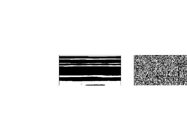
Figure 1: Snapshot configurations corresponding to the two phases of the Ising model with shear. On the left panel we observe a typical stripe-like configuration at $T<T_{c}$. On the right panel a configuration at $T>T_{c}$ is displayed. The external field is applied along the horizontal axis.

Previous theoretical and experimental studies have shown that sheared binary systems undergo a second order phase transition at a critical temperature $T_{c}$ [6]. In diffusive systems the effect of the external driving field is to inhibit fluctuations so that the critical temperature is expected to increase with the magnitude of the driving. In a continuum model with non–conserved dynamics, in the large-$N$ analytical approximation, it has been found that the value of the critical temperature depends on the driving field following a power law at small field magnitudes [7]. In previous Monte Carlo studies on the critical behavior of sheared Ising models [8], it was not possible to extract information about the critical temperature, due to numerical uncertainties and finite size effects [9]. In view of this, we revisit this issue, in order to determine the critical temperature of the model as a function of the magnitude of the external field, and to compute for the first time the critical exponents in this model. For the sake of comparison, we will contrast the obtained values with those computed for the 2d driven lattice gas model (DLG) [10] that will be briefly described in the next section.

To study the phase transition in the model, the critical dynamical behavior will be investigated by monitoring the time evolution of some observables before the system reaches nonequilibrium steady states (NESS). This technique, generally called short time dynamics [11, 12] is an alternative convenient way to obtain both the critical temperature and exponents precisely, with less computational cost than other methods commonly used, such as the finite size scaling applied to the specific heat and response functions, that require a considerably amount of simulation time in order to reach NESS. Furthermore, since the measurements are carried out in the first steps of evolution, the short time dynamic approach is free of the critical slowing down.

The manuscript is organized as follows: In Section 2, the Ising model with the external shear field is introduced. The technique used to study the phase transition is described in Section 3. The simulation results are presented in Section 4, and finally the conclusions are stated in Section 5.

2 The model

We will consider the nearest–neighbor two–dimensional Ising model with a single–spin–flip thermalization dynamics, e.g. the Metropolis dynamics [13]. The driving field will be defined in order to mimic the convective velocity shear profile

$$v_{x}(y)=\dot{\gamma}y\qquad v_{y}=0$$ (1)

where the parameter $\dot{\gamma}$ is called the shear rate and represents the shear field magnitude. If the system is imagined as a sequence of layers labelled by $y$, then $\dot{\gamma}y$ is the displacement of the layer $y$ in a unit of time. If $L_{y}$ is the vertical size and $v_{\textrm{max}}$ is the speed of the fastest layer, then $\dot{\gamma}L_{y}=v_{\textrm{max}}$.

The model is defined on a square lattice $\Lambda$ of horizontal and vertical sizes $L_{x}$, $L_{y}$ respectively, with periodic boundary conditions in the $L_{x}$ direction and free in the $L_{y}$ direction. More precisely, let $\Omega=\{-1,+1\}^{\Lambda}$ be the space of configurations and, for $\sigma\in\Omega$, let $\sigma_{x,y}$ be the value of the spin associated to the site $(x,y)\in\Lambda$. Then the Hamiltonian of the model is

$$H_{\Lambda}(\sigma)=-J\sum_{y=1}^{L_{y}}\sum_{x=1}^{L_{x}}\sigma_{x,y}\sigma_{x+1,y}-J\sum_{x=1}^{L_{x}}\sum_{y=1}^{L_{y}-1}\sigma_{x,y}\sigma_{x,y+1}$$ (2)

with $\sigma_{L_{x}+1,y}=\sigma_{1,y}$ for all $y=1,\dots,L_{y}$, and $J$ is a positive real coupling constant, which means that the interactions are ferromagnetic. We will combine the thermalization dynamics with an algorithm introducing the shear in the system. The shear is superimposed to the thermalization dynamics with typical rates not depending on the thermalization phenomenon, but fixed a priori. This has been done in different ways in [3, 8, 14]. In this paper we use a very ductile generalization of those dynamics aiming to introduce the shear effects in a way resulting competitive with respect to the thermalization process. Notice that our dynamics results from the combination of two steps: i) a thermalization step which would bring the system in the usual equilibrium; ii) a shear step which changes the configurations of the system forbidding to reach the equilibrium. Therefore, all together, our algorithm does not satisfy local detailed balance expressed in terms of standard equilibrium probabilities of configurations. Similar models have been also used in different context of non-equilibrium studies [15].

Let the time unit be the time needed for a full thermal update of the entire lattice, e.g. a full sweep of the Metropolis algorithm. The shear algorithm is parametrized with a submultiple $\tau$ of $L_{y}L_{x}$ (the period of the shear procedure), a positive integer $\lambda\leq L_{x}/2$ (the number of unit cells that a row is shifted when the shear is performed), and a non–negative real $\nu\leq 1/L_{y}$. The dynamics of the model that we study in this paper is defined in a precise way via the following algorithm:

1. set $t=0$, choose $\sigma_{0}\in\Omega$, and set $n=0$;

2. increase by 1 the index $n$, and choose at random with uniform probability $1/L_{x}L_{y}$ a site of the lattice and perform the elementary single–site step of the thermalization dynamics;

3. if $n$ is multiple of $\tau$ a layer is randomly chosen with uniform probability $1/L_{y}$. Then, if $\bar{y}$ is the chosen layer, all the layers with $y\geq\bar{y}$ are shifted by $\lambda$ lattice spacings to the right with probability $\nu L_{y}$;

4. if $n<L_{x}L_{y}$ goto 2, else denote by $\sigma_{t+1}$ the configuration of the system;

5. set $t=t+1$, set $n=0$, and goto 2.

We note that if $\nu=1/L_{y}$ the shift at step 3 is surely performed and this case will be later addressed to as full shear. The smoothness of the shear field, eqs. (1), is ensured by the random choice of the layer $\bar{y}$ in step 3. Now we want to express the shear rate $\dot{\gamma}$, introduced in equation (1), in terms of the parameters of our dynamics. We have to estimate the typical displacement per unit of time of the row labelled by $y$. Such a row is involved in a shear event, step 3 of the algorithm above, if and only if the extracted row $\bar{y}$ is such as $\bar{y}\leq y$, and this happens with probability $y/L_{y}$. Since the shear event results in a shift with probability $\nu L_{y}$, the probability that during a shear event the row $y$ does shift is given by

$$\frac{y}{L_{y}}\times\nu L_{y}=\nu y.$$

By noting that the number of shift events per unit of time is equal to $L_{x}L_{y}/\tau$ and recalling that the shift amplitude is $\lambda$, we have that the typical shift of the row $y$ per unit of time is given by

$$\frac{L_{x}L_{y}}{\tau}\times\lambda\times\nu y.$$

By using definition (1) we finally get $\dot{\gamma}=L_{x}L_{y}\nu\lambda/\tau$, which becomes $\dot{\gamma}=L_{x}\lambda/\tau$ in the case of full shear.
It is important to remark that there exists a large variety of models that evolve under non equilibrium states by the action of an external field. An example is the driven lattice gas (DLG) where the driving field is not superimposed to the thermalization dynamics, but it is rather inserted in the Metropolis transition rates, that become anisotropic, and biases the movement of particles along its direction [10]. Furthermore, it exhibits a second order phase transition at particle density $\rho=1/2$, between an ordered phase at low temperatures characterized by regions of low and high particle density, called stripes, oriented along the field direction, and a disordered phase at high temperatures with the appearance of a lattice gas. Both ordered and disordered phases have a similar appearance with those exhibited in figure 1. The critical temperature increases with the magnitude of the external field, saturating at $T_{c}\sim 1.41T_{c}(0)$ in the case of infinite [10]. Here, $T_{c}(0)=2.269$ $J/k_{B}$ is the critical temperature of the 2d Ising model ($J$ is the coupling constant and $k_{B}$ is the Boltzmann constant).

3 Dynamical Critical Behavior

It is known that, for systems exhibiting critical behavior, the relevant observables measured in equilibrium stationary states can be written in terms of power laws, with characteristic critical exponents due to the divergence of both the spatial correlations and the correlation time. In recent years, however, the attention has been also focused to the early stages of the evolution of the system towards the critical state, that is, to a microscopic time regime where the spatial correlation length is small compared with the system size [11]. Within this regime, it is possible to measure scaling laws of the observable quantities [12, 16]. This new method to study second-order phase transitions, called short time dynamics, allows to estimate the critical temperature and to compute the critical exponents of the transition with relative quickness and avoids the shortcomings that more usual techniques present to study critical behavior. Furthermore, the short time dynamics has been applied to investigate the critical behavior of a wide range of systems of different nature, such as models showing criticality under equilibrium conditions, such as e.g, the XY systems [17], the 2d 3-state Potts model [18], the Ising magnet under different lattice geometries [19, 20], and of nonequilibrium critical models such as the driven diffusive lattice gas (DLG) [21, 22, 23], etc. In these last three works, a detailed analysis of the second-order [21, 22] and first-order [23] non-equilibrium phase transition was performed by using the short time critical dynamic methodology. For the second-order phase transition, the excellent agreement between critical exponents evaluated using the standard (stationary) and dynamical (short time) approaches strongly support the robustness of this method. Encouraged by this success, our goal is to extend the short time dynamics concept to this model, basing our ideas on the already developed short time dynamics method for the DLG model in ref. [21].
The above mentioned scaling laws can be observed employing two different initial configurations, namely: 1) Fully disordered configurations (FDC’s), which means that the system is initially placed in a thermal bath at $T\rightarrow\infty$ , and the system configuration is similar to that exhibited on the right panel of figure 1; 2) Completely ordered configurations or ground state configurations (GSC’s) as expected for $T=0$. In our model, based on the fact that the equilibrium Ising model has all the spins pointing in the same direction (i. e. magnetization $M=$ 1 or -1) at this temperature, we will adopt this configuration as the ground state for testing the short time dynamic behavior.
The shear field introduces anisotropic effects, that generates anisotropic correlations in the system. As a consequence of this, there will be two correlation lengths, namely: 1) A parallel or longitudinal correlation length $\xi_{\parallel}$ along the external field direction, and 2) A perpendicular or transverse correlation length $\xi_{\perp}$ perpendicular to $\xi_{\parallel}$. Whatever the initial condition is used to start the system, both spatial correlation lengths are quite small or zero at the beginning of the dynamic process, and near the critical temperature $T_{c}$ they increase dynamically as a power law $\xi_{\parallel(\perp)}\propto t^{1/z_{\parallel(\perp)}}$, where $z_{\parallel(\perp)}$ is the dynamic critical exponent in the respective directions.
Before we start to describe the theoretical basis of the technique applied to this model, we set the external driving field along the horizontal direction, i.e. the $x$ axis. Also, we need to define quantities that are relevant in the critical behavior of the model. Based on the morphological appearance of typical configurations present in the system (see figure 1), we will consider a variant of the order parameter $OP$ employed in the critical study of the DLG model [21]:

$$OP=\frac{1}{L_{y}}\sum_{y=1}^{L_{y}}|P(y)|,$$ (3)

where $P(y)=\frac{1}{L_{x}}\sum_{x=1}^{L_{x}}\sigma_{x,y}$ is the average of the spin profile in the shear field axis.

The order parameter defined in this way can take into account the small ordering that appears at the early stages of the evolution.
There is one more point to take into account before we start to expose the method applied to this system. In all formulas below we will assume, and demonstrate later, that only the parallel correlation length is relevant in the short time critical evolution of the system. In fact at $T\simeq T_{c}(\dot{\gamma})$ and at early times of evolution, parallel and perpendicular correlations begin to increase. However, domains of perpendicularly correlated spins are broken by the shear, and assume a characteristic elongated shape, also observed in many experimental studies of sheared systems. As a consequence of this, transversal correlations grow slower than parallel correlations, so they do not take part in the dynamic critical behavior of the model at short times. This effect was also shown for the DLG model [21, 22]. Since this happens independently of the initial configuration, we will take $z=z_{\parallel}$ in every expression below. Furthermore, they must contain the anisotropic finite size dependence in order to match the usual anisotropic scaling forms for the NESS regime.
Starting with FDC’s, the scaling law proposed for the order parameter ($OP$) reads [21],

$$OP(t,\phi,L_{x},L_{y})=b^{-\beta/\nu_{\parallel}}OP^{*}(b^{-z}t,b^{1/\nu_{\parallel}}\phi,b^{-1}L_{x},b^{-\nu_{\perp}/\nu_{\parallel}}L_{y}),$$ (4)

where $t$ is the time, $b$ is the spatial rescaling factor, $\beta$ is the critical exponent of the order parameter, $\nu_{\parallel(\perp)}$ are the correlation length critical exponents in the $x$($y$) axis ($\xi_{\parallel(\perp)}\propto\phi^{-\nu_{\parallel(\perp)}}$), $OP^{*}$ is a scaling function, $z$ is the already mentioned dynamic exponent of the longitudinal correlation length, and $\phi=\frac{T-T_{c}}{T_{c}}$ . Notice also that $L_{y}$ is rescaled by $b^{-\nu_{\perp}/\nu_{\parallel}}$ to include possible shape effects in the dynamic critical behavior [10].
To generate the FDC initial conditions, the lattice is filled at random with exactly $\rho_{0}L_{x}L_{y}$ particles, being $\rho_{0}=1/2$ the density of up spins. However, the number of particles on each row parallel to the field axis is not the same for all rows. This generates tiny density fluctuations along this direction, which are of the order of $(1/L_{x})^{-\frac{1}{2}}$, in agreement with the central limit theorem. According to equation (4), these fluctuations add up, and the amplitude of $OP$ depends on $L_{x}^{-1/2}$. We have to take into account this expression for the final form of the time evolution of $OP$. Setting $b\simeq t^{1/z}$, eq. (4) becomes:

$$OP(t,\phi,L_{x},L_{y})=t^{-\beta/\nu_{\parallel}z}OP^{*}(1,t^{1/\nu_{\parallel}z}\phi,t^{-1/z}L_{x},t^{-\nu_{\perp}/\nu_{\parallel}z}L_{y}).$$ (5)

Then, if $t^{-1/z}L_{x}$ is extracted out of the scale function in Eq. (5), we have:

$$OP(t,\phi,L_{x},L_{y})=t^{-\beta/\nu_{\parallel}z}(t^{-1/z}L_{x})^{x}OP^{**}(1,t^{1/\nu_{\parallel}z}\phi,t^{-\nu_{\perp}/\nu_{\parallel}z}L_{y}),$$ (6)

but since $OP\simeq 1/L_{x}^{\frac{1}{2}}$, then $x=-1/2$, so, the final expression for $OP(t)$ is the following:

$$OP(t,\phi,L_{x})=L_{x}^{-1/2}t^{c_{1}}OP^{**}(t^{1/\nu_{\parallel}z}\phi)\qquad L_{x},L_{y}\rightarrow\infty,\qquad$$ (7)

with $c_{1}=(1-2\beta/\nu_{\parallel})/2z$ [21].

Furthermore, it is easy to show that the logarithmic derivative of $OP$ with respect to $\phi$, given by Eq. (7) at criticality, behaves as

$$\partial_{\phi}lnOP(t,\phi)\propto t^{c_{2}},\qquad\\$$ (8)

where the exponent is $c_{2}=1/\nu_{\parallel}z$.
On the other hand, starting the system from the GSC configuration described above, and according to the scaling behavior proposed in [21], we have

$$OP(t,\phi,L_{x},L_{y})=b^{-\beta/\nu_{\perp}}OP^{***}(b^{-z}t,b^{1/\nu_{\perp}}\phi,b^{-1}L_{x},b^{-\nu_{\parallel}/\nu_{\perp}}L_{y}),$$ (9)

where $OP^{***}$ is another scaling function . Here we have also included the shape scaling factor $b^{-\nu_{\perp}/\nu_{\parallel}}L_{y}$. Proceeding in the same way as in the above case, we have, taking $b\simeq t^{1/z}$ in (9) at criticality, the following expression for $OP$:

$$OP(t)\propto t^{-c_{3}}\qquad L_{x},L_{y}\rightarrow\infty,\qquad$$ (10)

with an exponent $c_{3}=\beta/\nu_{\perp}z$. Moreover, the derivative of Eq. (10) with respect to $\phi$ at criticality is given by

$$\partial_{\phi}OP(t)\propto t^{c_{4}},\qquad$$ (11)

where the exponent is $c_{4}=(1-\beta)/\nu_{\perp}z$.

4 Simulation Results

4.1 Critical Temperature

In this work we used rectangular and square lattices of different sizes $L_{x},L_{y}$, in the range $128\leq L_{x},L_{y}\leq 10000$ lattice units. The critical dynamics of the model was investigated as a function of the shear magnitude, in the range $1/32\leq\dot{\gamma}\leq 50$. The temperatures were measured in units of $J/k_{B}$, $k_{B}$ being the Boltzmann constant, and the time is measured in Monte Carlo steps (mcs), where one unit consists of $L_{x}L_{y}$ attempts for spin updates. The time evolution was sampled from 100 to 1000 realizations of the system, according to each initial condition and temperature.
We begin showing our results by considering the critical dynamic evolution of the system when it is started from FDC configurations, and then coupled with a thermal bath at $T\simeq T_{c}$. In figure 2, the time evolution of $OP(t)$ is shown for a system where a shear field is applied with shear rate $\dot{\gamma}=5$. The best power law behavior is obtained at $T=T_{c}=2.660$ before $OP(t)$ reaches a saturation value due to finite size effects. On the other hand, if $T<T_{c}$ or $T>T_{c}$, $OP$ deviates from the power law behavior as equation (7) states, and the curve shows an upward or downward bending, respectively (see the curves corresponding to $T=2.655$ and $T=2.665$ in the same figure)

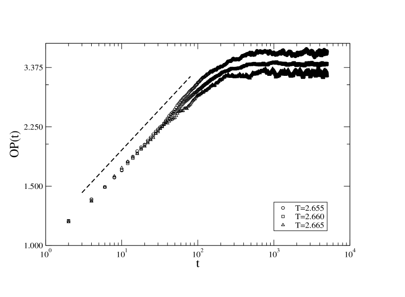
Figure 2: Log-log plot of the short time evolution of $OP(t)$ starting from FDC configurations, in a system with $L_{x}=L_{y}=512$ and $\dot{\gamma}=5$. The best fit of the raw data gives a power law behavior at $T_{c}=2.660$, as it is indicated by the dashed straight line. Upward and downwards deviations from this behavior can also be observed for $T=2.655$ and $T=2.665$, respectively.

The critical dynamic evolution was investigated by performing simulations also on rectangular lattices. The plots in figures 3 display the dynamic evolutions of $OP(t)$ at $T=T_{c}$ for two shear field magnitudes, $\dot{\gamma}=1/2$ and $\dot{\gamma}=10$ in a) and b) panels, respectively. The lattice sizes used are indicated in the legend of each plot by the notation $L_{x}$ $\times$ $L_{y}$. In the main plots of each figure, all early-time evolution exhibits the same power-law behavior with similar values of the exponent $c_{1}$ (equation (7)). Then, a saturation value is reached, $OP_{sat}$, that depends only on $L_{x}$, as it can be observed in lattices with longitudinal sizes $L_{x}=500$ and $L_{x}=1000$ for $\dot{\gamma}=1/2$ and $L_{x}=500$ for $\dot{\gamma}=10$ respectively. So, these plots show that the early-time critical evolution of the system is free from lattice shape effects [10], because the relation between the longitudinal and transversal sizes is different for each studied case. The same was observed in the short-time critical evolution of the DLG model [21]. In addition, the power law behaviors can be collapsed by rescaling $OP(t)$ by $L_{x}^{1/2}$ as it is proposed in equation (7). This is shown in the insets of both figures

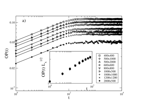
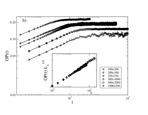
Figure 3: Log-log plots of the time evolutions of $OP(t)$ at $T=T_{c}$, for the system in rectangular and square lattices of sizes $L_{x}\times L_{y}$, as indicated in the legends. In a) the external field has magnitude $\dot{\gamma}=1/2$ while in b) the shear field magnitude is $\dot{\gamma}=10$. The straight lines are least-square fits of the data. The insets in each figure show the collapse of the power law behaviors when $OP(t)$ is multiplied by $L_{x}^{1/2}$

Then, the critical points of the system at several values of the shear field magnitudes $\dot{\gamma}$ were found. Figure 4 shows that the power-law behavior of $OP$ collapses for large values of $\dot{\gamma}$, i.e. $\dot{\gamma}=5,10$ and $50$, and occurs at approximately the same critical temperatures for each shear rate. These temperatures are larger than the estimated for the equilibrium Ising model, $T_{c}(\dot{\gamma}=0)=2.269$ (see table 1). However, the time evolution of $OP$ depends on the shear field if $\dot{\gamma}$ is small, as it can be seen for the cases $\dot{\gamma}=1/32$ and $\dot{\gamma}=1/10$. Although these magnitudes are quite small, they are enough to raise the critical temperature to $T_{c}(\dot{\gamma}=1/32)=2.29$ and $T_{c}(\dot{\gamma}=1/10)=2.395$, both close but greater than the critical temperature of the Ising model. This confirms that the critical temperature depends on the shear field magnitude, as found by theoretical studies [7].

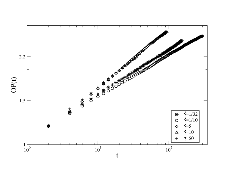
Figure 4: Log-log plots of the time evolutions of $OP(t)$ at $T=T_{c}$ corresponding to systems with different shear fields. The magnitudes $\dot{\gamma}$’ are indicated in the legend.

Once that the critical temperatures $T_{c}$ corresponding to the different $\dot{\gamma}$’s were collected, a diagram of critical temperatures versus $\dot{\gamma}$ can be performed. Figure 5 shows that two regimes can be distinguished. In the first regime, the critical temperature grows with $\dot{\gamma}$ as a power law, i. e. $T_{c}(\dot{\gamma})/T_{c}(0)-1$ $\propto$ $\dot{\gamma}^{\psi}$. The value of the exponent was estimated in $\psi=0.52(3)$, which is consistent with that calculated theoretically in [7]. In this work (ref. [7]), the critical transition in the $\varphi^{3}\rightarrow\langle\varphi^{2}\rangle\varphi$ approximation was studied in a scalar field model based on a convection-diffusion equation with Landau-Ginzburg free energy, with the average $\langle\varphi^{2}\rangle$ self-consistently determined. Above the lower critical dimension, the exponent $\psi$ was evaluated to be $1/2$ and $1/4$ for the cases with non-conserved and conserved order parameter respectively.

Then, $T_{c}$ crosses over to a saturation regime at larger $\dot{\gamma}$’s, saturating at $T_{c}(\dot{\gamma})\backsim 1.18T_{c}(0)$, where $T_{c}(0)\approxeq 2.269$ is the critical temperature of the 2D Ising model. The increase of the critical temperature by action of the external field, and a posterior saturation regime was also observed in the DLG model [10]. We want to remark also that in real fluids there is also a negative contribution to the shift of the critical temperature coming from hydrodynamics interactions [24]. The total shift of $T_{c}$ results to be negative for fluids with low molecular weight [24], was also found in experiments [25]. A review for other systems is given in [6].

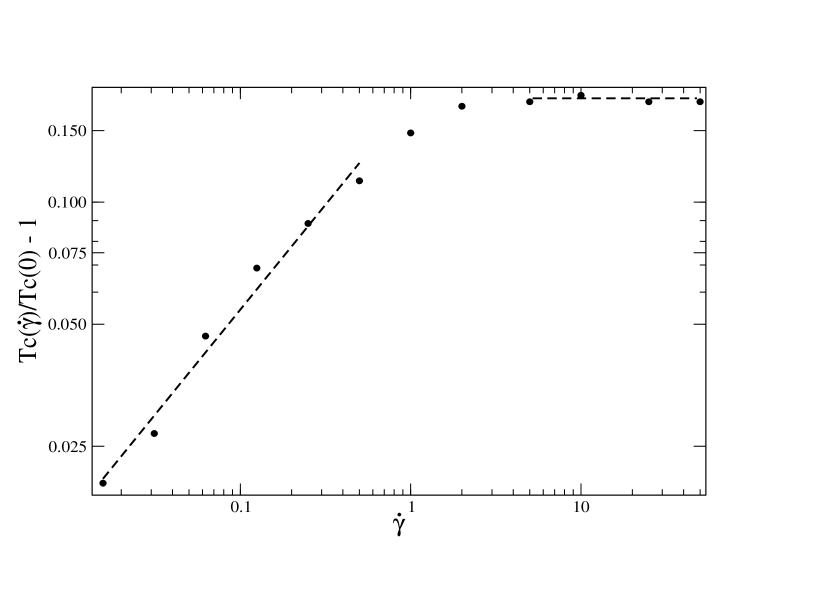
Figure 5: Diagram of critical temperatures $T_{c}(\dot{\gamma})/T_{c}(0)-1$ versus $\dot{\gamma}$, in log-log scale. The fit of the data points in the growing regime gives a slope $\psi=0.52(3)$.

On the other hand, if the system is started from the GSC initial condition (i.e. magnetization equal to 1), and then it is left to evolve at the working temperature $T\simeq T_{c}$, $OP(t)$ decreases, and follows a power law behavior at $T=T_{c}$. Upwards or downwards deviations are observed according if $T<T_{c}$ or $T>T_{c}$, respectively. Figure 6 exhibits the evolution of $OP(t)$ for the same parameters of figure 2. A clear power law behavior can be observed at $T=2.66$, which is exactly the same temperature found when the system was started from FDC configurations. This is precisely the signature of a second-order phase transition in the model. In addition, the expected deviations from the power law behavior at $T=2.65$ and $T=2.67$ are also observed.

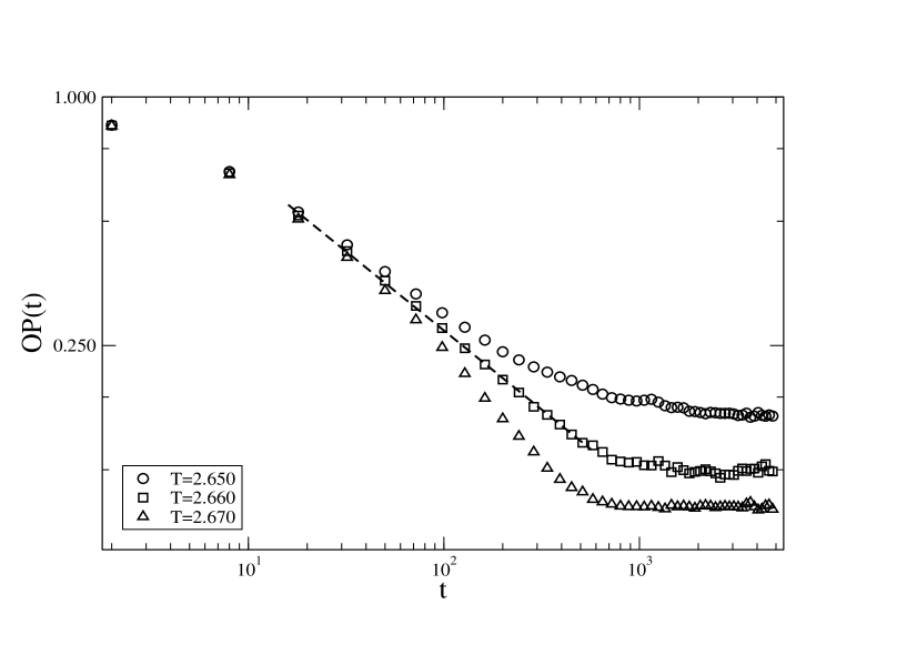
Figure 6: Log-log plot of the time evolutions of $OP(t)$ corresponding to a system set in a square lattice of size $L_{x}=L_{y}=512$ with shear rate $\dot{\gamma}=5$. The working temperatures of the thermal bath are indicated in the legend. A power law behavior is observed for $T_{c}=2.660$ $J/k_{B}$. The dashed line is a fit of the numerical data.

Proceeding in the same way we did for the evolutions started from FDC’s, the critical behavior of the system was investigated when it is started from GSC configurations in rectangular lattices. Figures 7 a) and b) show the critical time evolution of $OP$ when the system is initiated from a GSC configuration, corresponding to $\dot{\gamma}=1/2$ and $\dot{\gamma}=10$, respectively. It is important to remark that the best power law behavior was obtained when the systems evolved at the same critical temperatures found when they were initiated from FDC configurations. According to the results, the transversal size $L_{y}$ does not play a relevant role in the critical behavior of the system as it is shown in the evolutions in lattices with $L_{x}=500$ (figure 7 a) and b)) and also with $L_{x}=2000$ (figure 7 b)), but rather the longitudinal size $L_{x}$ is relevant. This is in agreement with the results previously exhibited in figure 3, and allow to conclude that that the critical evolution of the system is independent of lattice shape effects for both initial configurations.

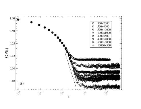
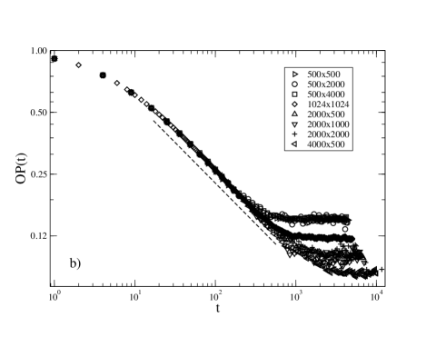
Figure 7: Log-log plots of the time evolutions of $OP(t)$ at $T=T_{c}$, for the system set in rectangular and square lattices of sizes $L_{x}\times L_{y}$, as indicated in the respective legends. In a) the external field has magnitude $\dot{\gamma}=1/2$ while in b) the shear field magnitude is $\dot{\gamma}=10$. The dashed lines displaced are least-square fits of the obtained data.

4.2 Critical Exponents

Focusing our attention on the power law behavior at the $T=T_{c}$, the exponents $c_{1}$ and $c_{2}$ corresponding to the dynamic evolution of $OP$ (equation (7)) and its logarithmic derivative $\partial_{\tau}lnOP(t,\tau)$ (equation (8)) can be estimated. Table 1 enlists the obtained values of $T_{c}$ and the mentioned exponents for small and large values of $\dot{\gamma}$. The values of $c_{1}$ and $c_{2}$, for the case of $\dot{\gamma}=1/32$ are different compared with the those at larger $\dot{\gamma}$, as it was already observed in figure 4. Furthermore, the value of $c_{1}$ for $\dot{\gamma}=50$ is also slightly different from the corresponding cases of $\dot{\gamma}=5$ and $\dot{\gamma}=10$. This seems to be a rare behavior, since there exists a saturation regime for the critical temperature at these values of $\dot{\gamma}$’s (figure 5), and we are induced to think that the dynamic behavior of the system is independent of the field magnitude in this limit. Opposite to that, the estimated values of $c_{2}$ are quite similar in the limit of large $\dot{\gamma}$’s.

$\dot{\gamma}$	$T_{c}$	$c_{1}$	$c_{2}$
1/32	2.29	0.180(8)	0.99(2)
5	2.66	0.239(1)	0.84(1)
10	2.675	0.238(1)	0.87(1)
50	2.675	0.224(1)	0.85(1)

Table 1: Exponents $c_{1}$ and $c_{2}$, obtained from FDC initial conditions, corresponding to the values of $\dot{\gamma}$ enlisted in the first column.

Table 2 enlists the values of the exponents $c_{3}$ and $c_{4}$ that were obtained from a least-square fits of the critical evolution of the system when it is initiated from the GSC configurations (see equations (10) and (11)). Here, the same situation that happened for $c_{1}$ is found for $c_{3}$. In fact, the value of $c_{3}$ for $\dot{\gamma}=1/32$ is different form the rest of the corresponding values at larger $\dot{\gamma}$’s, and the value of $c_{3}$ for $\dot{\gamma}=50$ is also different from the values estimated for $\dot{\gamma}=5$ and $\dot{\gamma}=10$. On the other hand, the values of $c_{4}$ are similar for all the reported cases of $\dot{\gamma}$’s.

$\dot{\gamma}$	$T_{c}$	$c_{3}$	$c_{4}$
1/32	2.29	0.076(1)	0.65(2)
5	2.66	0.401(1)	0.63(1)
10	2.675	0.405(5)	0.62(1)
50	2.675	0.360(7)	0.62(5)

Table 2: Exponents $c_{3}$ and $c_{4}$ obtained from the GSC configuration, corresponding to the values of $\dot{\gamma}$ enlisted in the first column.

According to the equations developed in section 3, the critical exponents of the second-order phase transition, are obtained by combining the estimated exponents $c_{1}$, $c_{2}$, $c_{3}$, and $c_{4}$ enlisted above, corresponding to each case of $\dot{\gamma}$ investigated. Table 3 resumes the obtained results and includes the critical exponents of both the Ising and DLG model for the sake of comparison. Since this issue for the case of the DLG model still remains an open problem, the obtained theoretical values from all proposed theories exposed in refs. [10] and [27] are included.

$\dot{\gamma}$	$\beta$	$z$	$\nu_{\perp}$	$\nu_{\parallel}$
1/32	0.105(1)	1.77(7)	0.78(1)	0.57(5)
5	0.39(1)	0.88(1)	1.10(1)	1.35(2)
10	0.39(1)	0.86(1)	1.14(1)	1.34(1)
50	0.37(1)	0.94(1)	1.10(1)	1.30(6)
Ising 2d	0.125	2.16	1	1
DLG(E=50) (ref. [10])	1/2	$\approx$4/3	$\approx$3/2	$\approx$1/2
DLG (E=50) (ref. [27])	$\approx$0.33	$\approx$1.998	$\approx$1.22	$\approx$0.63

Table 3: Table of the calculated critical exponents for each case of $\dot{\gamma}$ employed. The critical exponents corresponding to both theories of the critical phase transition of the Ising and the DLG models are also included for comparison. Since there is no anisotropy in the Ising model $\nu_{\bot}=\nu_{\parallel}=\nu$ must be read. The results of this table do not fit with the relation $\psi=1/\nu z$ suggested in [24]. See, however, in Sect. 5, the discussion about our results our small shear rates.

An overview of this table deserves some comments. First, the calculated value of $\beta$ at $\dot{\gamma}=1/32$ is close to $\beta=1/8$ calculated for the 2d Ising model. This similarity could drive us to think that the effects of the shear field are negligible, but this is not the case, as it is evidenced by the values of the rest of the critical exponents. In fact, anisotropy effects are important, even if a small external field, in this case $\dot{\gamma}=1/32$, is applied. The dynamic exponent $z(\dot{\gamma}=1/32)=1.77(7)$ indicates that the correlation length (in the longitudinal direction, see 4.3) grows faster with time than the corresponding one in the Ising model $z=2.16$, and the difference between $\nu_{\bot}(\dot{\gamma}=1/32)=0.78(1)$ and $\nu_{\parallel}(\dot{\gamma}=1/32)=0.57(5)$ reveals an anisotropic critical behavior even at small shear rate values.
The situation is different for the critical exponents at the largest values of $\dot{\gamma}$ investigated. The values of the exponents are similar between each other, suggesting that the critical behavior does not depend of the applied field. This fact is also present in figure 5, where the critical temperature is approximately the same for the largest values of $\dot{\gamma}$ used. Furthermore, we also noticed that $\nu_{\bot}>\nu_{\parallel}$ for $\dot{\gamma}=1/32$, while it happens the opposite at large $\dot{\gamma}$. At the moment, a reasonable explanation for this issue is not possible due to the lack of a theoretical framework about the critical behavior of this model.
To end this section, one final comment is appropriate. In view of the values exposed in table 3, the computed critical exponents do not belong to the universality classes of the Ising or of the DLG models respectively. This fact is not surprising since, as we have seen, the shear rate affects the critical behavior of the model by inducing anisotropic effects in the equilibrium model that changes its behavior. The case of the DLG model is different. Although both models have a similar phase behavior, the particle dynamics defined for the DLG model conserves the number of particles while our model does not. This difference will probably affect the values of the critical exponents, and in consequence there is no reason to expect that both models will belong to the same universality class.

4.3 Longitudinal Correlation

In section 3, it is assumed that the dynamic increase of the longitudinal correlation length $\xi_{\parallel}$ and the breakage of the corresponding transversal one $\xi_{\perp}$ at $T=T_{c}$ are due to the anisotropy effects induced by the external shear field. This will cause that the short-time critical dynamic evolution of the system initiated from either the FDC or GSC configurations will depend only on the dynamic critical exponent $z_{\parallel}=z$ that describes the critical dynamic increase of $\xi_{\parallel}$.
To show our hypothesis, we performed a scaling of the whole curve of the $OP(t)$ for the cases of $\dot{\gamma}=1/2$ (small driving field) and $\dot{\gamma}=10$ (large driving field). We propose a phenomenological scaling in the spirit of the scaling form used by Family and Vicsek to describe the roughness growth of interfaces [26] (obviously in a different context not related to ours). This is given by the following expression

$$OP=L_{x}^{-\omega_{i}}f(t/L_{x}^{z}),$$ (12)

where $L_{x}$ is the longitudinal size, according to the results exhibited in figures 3 and 7 a) and b), respectively. The exponent $\omega_{i}$, $i=$FDC or GSC, is the exponent that has into account the finite-size critical behavior of $OP$, and $z$ is the relevant dynamic critical exponent. The idea of this scaling form is simple: if all the curves can be collapsed by using the same dynamic exponent $z$ independently of the initial condition used to start the simulations, it can be demonstrated numerically that only one correlation is relevant in the critical dynamic behavior. Furthermore, equation (12) must contain both the critical dynamic behavior of $OP$ according to equations (5) and (10) at the early times of evolution, and the finite size behavior in the limit of large times ($t\rightarrow\infty$) where the correlation length is comparable to $L_{x}$. Therefore we have that $f(u)$ must be $f\propto(t/L_{x}^{z})^{-\beta/\nu_{\parallel}z}$ or $f\propto(t/L_{x}^{z})^{-\beta/\nu_{\perp}z}$ at early times $u\ll 1$, depending if the initial condition is $FDC$ or $GSC$ respectively. This fixes the finite-size exponent $\omega_{i}$ in $\omega_{FDC}=\beta/\nu_{\parallel}$ or $\omega_{GSC}=\beta/\nu_{\perp}$ according to the initial configuration used to start the simulations.
Figures 8 and 9 a) and b) exhibit both the finite-size dependence of $OP(t)$ with the longitudinal size $L_{x}$ (insets), and the scaling function $f(t/L_{x}^{z})$ (main plots), for the small and large external fields, represented by $\dot{\gamma}=1/2$ (figures 8) and $\dot{\gamma}=10$ (figures 9) respectively. In all plots, the finite-size dependence is obtained by calculating the saturated value of $OP(t)$, $OP_{sat}$, from figures 3 and 7, which were plotted versus $L_{x}$.

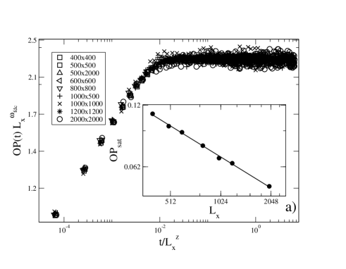
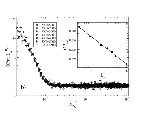
Figure 8: Log-log plots of the scaling functions $f(t/L^{z})$ (see equation (12)) of the time evolution of $OP(t)$ when the system is started from FDC and GSC configurations (main plot of figure a) and b) respectively) corresponding to a system with external field of magnitude $\dot{\gamma}=1/2$. The insets of both figures show the finite-size dependence and the corresponding power-law fit in a double logarithmic scale. The values of the corresponding fits are $\omega_{FDC}=0.50(1)$ (inset of a) ) and $\omega_{GSC}=0.53(1)$ (inset of b)), respectively.

As it can be observed in the insets of the plots in figures 8 a) and b) the size dependence of $OP$ in the long time regime can be well fitted by a power law as it is proposed in equation (12). The estimated exponents $\omega_{fdc}=0.50(1)$ and $\omega_{gsc}=0.53(1)$ were not consistent with the expected values $\omega_{FDC}=\beta/\nu_{\parallel}=0.263(3)$ or $\omega_{GSC}=\beta/\nu_{\perp}=0.242(2)$. However, the good collapses performed with the same $z(\dot{\gamma}=1/2)=1.45(3)$ exhibited in the main plots of both figures clearly evidences that only longitudinal correlations are relevant in the critical evolution of the system at short times.

On the other hand, the insets of figure 9 a) and b), show that the finite-size behavior of $OP(t)$ is also a power law for the case of large shear field magnitudes, represented by $\dot{\gamma}=10$. Opposite to the case with $\dot{\gamma}=1/2$, the estimated values of $\omega_{fdc}=0.29(2)$ and $\omega_{gsc}=0.34(3)$ were in agreement with the expected values $\omega_{FDC}=\beta/\nu_{\parallel}=0.291(2)$ or $\omega_{GSC}=\beta/\nu_{\perp}=0.342(2)$ calculated from Table 3. The good collapses performed with $z(\dot{\gamma}=10)$ displayed in the main plots of the figures allow us to conclude that the same behavior observed for small $\dot{\gamma}^{\prime}s$ is also exhibited by systems with large values of the external fields.

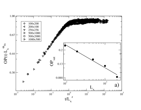
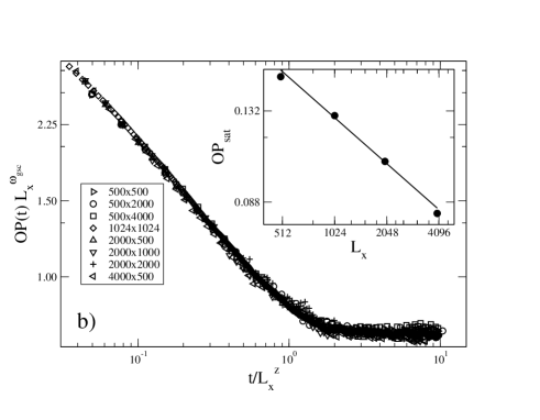
Figure 9: Log-log plots of the scaling functions $f(t/L^{z})$ (see equation (12)) of the time evolution of $OP(t)$ when the system is started from FDC’s and GSC’s configurations (main plot of figure a) and b) respectively) corresponding to a system with external field of magnitude $\dot{\gamma}=10$. The insets of both figures show the finite-size dependence and the corresponding power-law fit in a double logarithmic scale. The values of the corresponding fits are $\omega_{fdc}=0.29(2)$ (inset of a) ) and $\omega_{gsc}=0.34(3)$ (inset of b)), respectively.

To summarize. we have shown that the critical dynamic evolution of the system, started from either FDC’s or GSC initial configurations, can be scaled with the dynamic critical exponent $z$ proposed in Section 3. Based on the arguments exposed in Section 3, we can conclude that, in the short time limit of the critical evolution, the correlations along the field axis (longitudinal) are more relevant than transverse (perpendicular) correlations. Furthermore, the obtained finite-size exponents $\omega_{i}$ are only in accordance with those calculated using the critical exponents enlisted in Table 3 corresponding to $\dot{\gamma}=10$, while at $\dot{\gamma}=1/2$ they differ by a factor of nearly 2.

5 Discussion and Conclusions

In this work, the second-order phase transition in the 2d non-conserved Ising model under the action of an external driving shear field was investigated by studying the critical evolution of the system in the short-time regime. In order to apply this method, the dynamic evolution of the system at $T\simeq T_{c}(\dot{\gamma})$ was monitored when it is initiated from fully disordered initial configurations (FDC), and from the completely ordered configuration (GSC).

Starting the system from FDC’s configurations, the time evolution of the order parameter $OP$ follows a power law behavior at the critical temperature $T_{c}$, while at slightly different values of $T$ the power law is modulated by a scaling function that bends upwards or downwards depending if the temperature is less or greater than $T_{c}$, respectively. The critical evolution was studied on square and rectangular lattices of different sizes $L_{x}$ and $L_{y}$, and the results indicate that the short-time critical evolution is free of shape effects. Furthermore, the saturation value reached by $OP$ depends only on $L_{x}$. The critical evolution started from FDC’s configurations was studied for different values of $\dot{\gamma}$, and the diagram of reduced temperatures $T_{c}(\dot{\gamma})/T_{c}(0)-1$ versus $\dot{\gamma}$, $T_{c}(0)=2.269$ $J/k_{B}$ was drawn. As a first observation, all the values found for $T_{c}(\dot{\gamma})$ are always greater than the 2d critical temperature of the Ising model, that is typical for models driven out of equilibrium by an external field. Furthermore, two regimes can be distinguished: 1) a growing regime where $T_{c}(\dot{\gamma})/T_{c}(0)-1$ $\propto$ $\dot{\gamma}^{\psi}$. The exponent $\psi$ was calculated by means of a linear regression fit, giving $\psi=0.52(3)$, which is consistent with theoretical predictions in ref. [7]; 2) a saturation regime, where $T_{c}(\dot{\gamma})$ does not change appreciably with $\dot{\gamma}$. In this regime $T_{c}(\dot{\gamma})\sim 1.18T_{c}(0)$. A similar diagram was already observed in the DLG model [10], where the temperature grows with the magnitude of the driving field and then saturate at large values.
On the other hand, the critical dynamic behavior of the model was also investigated when it is initiated from the ground state configuration (GSC). A decreasing power law is observed for $OP(t)$ at the same $T_{c}(\dot{\gamma})$ found when the system was started from FDC configurations. This evidences that the model experiences a second order phase transition, as expected. Also in this case, the critical evolution of the system was simulated on rectangular and square lattices of different sizes. It was found that the critical evolution is independent of the shape of the lattice and the saturation value of $OP$ only depends on the longitudinal size $L_{x}$, as for evolutions initiated from FDC configurations. So, it is concluded as a general result that in the short-time scale, the system critical evolution is free of shape effects, as it is also observed for the critical evolution of the DLG model in the same time interval [21].

Then, the quantities $c_{i}$ ($i=1,4$), defined in sect. 3, were studied in order to calculate the critical exponents of the transition. Starting from FDC’s initial configurations, the dynamic critical behavior at small $\dot{\gamma}$ is slower than at larger $\dot{\gamma}$’s. As it can be observed in figure 2 and in Table 1, the order parameter exponent $c_{1}$ is smaller at $\dot{\gamma}=1/32$ than at larger $\dot{\gamma}$’s. Also, its logarithmic derivative exponent $c_{2}$ is different for this case. On the other hand, the values of $c_{1}$ and $c_{2}$ are more stable for larger $\dot{\gamma}$’s, although $c_{1}$ at $\dot{\gamma}=50$ is slightly smaller than the estimated values for $\dot{\gamma}=5,10$ . A similar scenario was found for the order parameter $c_{3}$ and its derivative $c_{4}$ exponents starting from the GSC configuration.
By combining these exponents, the static and dynamic critical exponents $\beta$, $\nu_{\bot}$, $\nu_{\parallel}$ and $z$ were calculated and are enlisted in table 3. The order parameter critical exponent $\beta$ for $\dot{\gamma}=1/32$ is similar to the value calculated for the Ising model, but the values of $z$, $\nu_{\parallel}$ and $\nu_{\bot}$ show that the anisotropy introduced by such a small external field is relevant. At large $\dot{\gamma}$’s, all the exponents are similar within a small range, suggesting that the critical behavior of the model is practically independent of the magnitude of the field in this regime. Furthermore, Table 3 also shows that the critical exponents of the sheared model do not belong to the universality class of the Ising or of the DLG model, even if this model shows a similar phase behavior.

Finally, the critical exponents summarized above were computed based on the fact that only the longitudinal correlation length is relevant for the dynamic critical behavior of the model, independently of the initial configuration. In order to check this, a finite-size scaling of the dynamic evolution of $OP$ was performed with the aid of equation (12). This equation must contain both the critical dynamic behavior of equations (5) and (10) at early times of evolution, and also the finite-size critical behavior at long times. As a consequence, the finite-size exponents must be $\omega_{FDC}=\beta/\nu_{\parallel}$ and $\omega_{GSC}=\beta/\nu_{\perp}$ for both initial conditions respectively. By measuring the saturated values of $OP$, $OP_{sat}$, and computing the exponents $\omega_{FDC}$ and $\omega_{GSC}$ the time series of $OP$ were collapsed for the system initiated from ordered and disordered configurations as the main plots of figures 8 and 9 show. Therefore, it is concluded that only the longitudinal correlation length $\xi_{\parallel}$ takes part in the critical evolution of the Ising model when an external shear field is applied. Furthermore, the finite-size exponents $\omega_{FDC}$ and $\omega_{GSC}$ were not consistent with the rates $\beta/\nu_{\parallel}$ and $\beta/\nu_{\perp}$ for the cases corresponding to $\dot{\gamma}=1/2$, while they are in good agreement for a shear field of magnitude $\dot{\gamma}=10$. This discrepancy between the predicted and measured critical exponents for the case $\dot{\gamma}=1/2$, together with the fact that the values of the critical exponents estimated for smaller $\dot{\gamma}$ are not similar with those corresponding to larger values of $\dot{\gamma}$ (see Table 3), may be explained by conjecturing that, at such small values of the shear rate, the system is less perturbed by the external driving. This means that the growth of transverse critical correlations is less affected by the shear field, and may become relevant in the short time regime. If this is so, our scaling assumptions will be not longer valid, and both $\xi$’s need to be considered in order to propose scaling forms for the dynamic critical behavior of the model in this regime. In order to study this, new simulations of the model with $\dot{\gamma}=1/32$ were performed, but they demanded a lot of computational time, specially when the system is started from the GSC configurations because they needed larger lattice sizes and evolution time intervals in order to obtain good power laws and saturation regimes ($L\geq 10000$, evolution time intervals of the order of $10^{6}$ MCS or larger), so we did not obtained reliable results. As a consequence, this interesting subject will be left for further research in the future. In contrast, at larger $\dot{\gamma}^{\prime}s$, the good agreement between $\beta/\nu_{\parallel}$ and $\beta/\nu_{\perp}$, calculated from the exponents in Table 3, and the estimated values of $\omega_{FDC}$ and $\omega_{GSC}$ respectively, suggest that the critical behavior is different from both the cases with smaller $\dot{\gamma}^{\prime}s$, and also from the Ising and DLG models at large external fields [21, 22].

6 Acknowledgements

GPS wants to thank CONICET and the ANPCyT.

References

- [1] See, e.g., A. J. Bray, Adv. Phys. 43, 357 (1994).
- [2] P. C. Hohenberg and B. I. Halperin, Rev. Mod. Phys. 49, 435 (1977).
- [3] A. Cavagna, A. J. Bray, and R. D. M. Travasso, Phys. Rev. E 62, 4702 (2000).
- [4] E. N. M. Cirillo, G. Gonnella, and G. P. Saracco, Phys. Rev. E 72, 026139 (2005).
- [5] R. G. Larson, The Structure and Rheology of Complex Fluids, (Oxford University Press, New York, 1998). (1991); N. Mason, A.N. Pargellis, and B. Yurke Phys. Rev. Lett. 70, 190 (1993); B. Yurke, A.N. Pargellis, S.N. Majumdar, and C. Sire, Phys. Rev. E 56, R40 (1997).
- [6] A. Onuki, J. Phys. Condens. Matter 9, 6119 (1997).
- [7] G. Gonnella, and M. Pellicoro, J. Phys. A: Math Gen. 33, 7043, (2000).
- [8] C. K. Chan, and L. Lin, Europhys Lett. 13, 13, (1990).
- [9] F. Corberi, G. Gonnella, and A. Lamura, Phys. Rev. Lett. 83, 4057 (1999).
- [10] See, e. g., B. Schmittmann and R. K. P. Zia, in Statistical Mechanics of Driven Diffusive System, in Phase transitions and Critical Phenomena, Vol. 17, edited by C. Domb and J. Lebowitz, Academic, London (1995).
- [11] H. K. Janssen, B. Schaub and B. Schmittmann, Z. Phys. B 73. 539 (1989).
- [12] B. Zheng, Int. J. Mod. Phys B 12 No. 14, 1419 (1998). Review article.
- [13] N. Metropolis, A. W. Rosembluth, M. N. Rosembluth, A. M. Teller and E. Teller, J. Chem. Phys. 21, 1087 (1953).
- [14] Y. Okabe, T. Miyajima, T. Ito, and T. Kawakatsu, Int. J. of Mod. Phys. C., 10 Number 8, 1513, (1999).
- [15] G. Crooks, Phys. Rev. E 61, 2361 (2000).
- [16] B. Zheng, Physica A 283, 80 (2000).
- [17] H. J. Luo, M. Schultz, L. Schülke, S. Trimper and B. Zheng, Phys. Lett A 250, 383 (1998).
- [18] B. Zheng, cond-mat/9705233.
- [19] L. Schülke and B. Zheng, Phys. Rev. E, 62 , 7482 (2000).
- [20] M. A. Bab, G. Fabricius and E. V. Albano, Phys. Rev. E, 71 , 036139 (2005).
- [21] E. V. Albano and G. Saracco, Phys. Rev. Lett. 88, 145701 (2002).
- [22] E. V. Albano and G. Saracco, Phys. Rev. Lett. 92 number 2, 029602 (2004).
- [23] G. P. Saracco and E. V. Albano, J. Chem. Phys, 118, No. 9, 4157 (2003).
- [24] A. Onuki and K. Kawasaki, Ann. Phys 121 Issues 1-2, 456 (1979).
- [25] D. Beysens, M. Gbadamassi and B. Mouncef-Bouanz, Phys. Rev. A, 28 number 4, 2491 (1983).
- [26] F. Family and T. Vicsek, J. Phys. A: Math. Gen. 18, L75 (1985).
- [27] P. L. Garrido, F. de los Santos and M. A. Muñoz, Phys. Rev. E 57, 752 (1998). P. L. Garrido, M. A. Muñoz and F. de los Santos, Phys. Rev. E. 61, R4683 (2000); F. de los Santos, P. L. Garrido and M. A. Muñoz, Physica A 296, 362 (2001).