Astrometry and photometry with HST-WFC3. I.            Geometric distortion corrections of F225W, F275W, F336W bands of the UVIS-channel.

Abstract

An accurate geometric distortion solution for the Hubble Space Telescope UVIS-channel of Wide Field Camera 3 is the first step towards its use for high precision astrometry. In this work we present an average correction that enables a relative astrometric accuracy of $\sim$1 mas (in each axis for well exposed stars) in three broad-band ultraviolet filters (F225W, F275W, and F336W). More data and a better understanding of the instrument are required to constrain the solution to a higher level of accuracy.

1 Introduction, Data set, Measurements

The accuracy and the stability of the geometric distortion (GD) correction of an instrument is at the basis of its use for high precision astrometry. The particularly advantageous conditions of the Hubble Space Telescope (HST) observatory make it ideal for imaging-astrometry of (faint) point sources. The point-spread functions (PSFs) are not only sharp and (essentially) close to the diffraction limit –which directly results in high precision positioning– but also the observations are not plagued by atmospheric effects (such as differential refraction, image motion, differential chromatic refraction, etc), which severely limit ground-based astrometry. In addition to this, HST observations do not suffer from gravity-induced flexures on the structures of the telescope (and camera), which add (relatively) large instabilities in the GD of ground-based images, and make its corrections more uncertain.

Last May 14, the brand-new Wide Field Camera 3 (WFC3) was successfully installed during the Hubble Servicing Mission 4 (SM4, May 12-24 2009). After a period of intense testing, fine-tuning, and basic calibration, last September 9th, 2009, the first calibration- and science-demonstration images were finally made public.

Our group is active in bringing HST to the state of the art of its astrometric capabilities, that we used for a number of scientific applications (e.g. from King et al. 1998, to Bedin et al. 2009, first and last accepted papers). Now that the “old” ACS/WFC is successfully repaired, and that the new instruments are installed, our first step is to extend our astrometric tools to the new instruments (and to monitor the old ones). This paper is focused on the geometric distortion correction of the UV/Optical (UVIS) channel of the WFC3. Since the results of these efforts might have some immediate public utility (e.g. relative astrometry in general, stacking of images, UV-identification of X-counterparts such as pulsars and CVs in globular clusters, etc.), we made our results available to the WFC3/UVIS user-community.

We immediately focused our attention on a deep UV-survey of the core of the Galactic globular cluster $\omega$ Centauri (NGC 5139), where some well dithered images were collected. The dense –and relatively flat– stellar field makes the calibration particularly suitable for deriving and monitoring the GD on a relatively small spatial scale. In addition, while most of the efforts to derive a GD correction will be concentrated on relatively redder filters, we undertook a study to determine the GD solutions of the three bluest broad-band filters (with the exception of F218W): F225W, F275, and F336W.

The WFC3/UVIS layout is almost indistinguishable from that of ACS/WFC: two E2V thinned, backside illuminated and UV optimized 2k$\times$4k CCDs contiguous on the long side of the chip, and covering a field of view (FoV) of $\sim 160$$\times$$160$ arcsec². The $\omega$ Cen data set used here consists of 9$\times$350 s exposures in each of the filters F225W, F275W, and F336W. The nine images follow a squared 3$\times$3 dither-pattern with a step of about 40 arcsec (i.e. $\sim$1000 pixels), and were all collected on July 15, 2009.

We downloaded the standard pipe-line reduced FLT files from the archive. The FLT images are de-biased and flat-field corrected, but no pixel-resampling is performed on them. The FLT files are multi-extension fits (MEF) on which the first slot contains the image of what –hereafter– we will call chip 1 (or simply [1]). The second chip, instead, is stored in the fourth slot of the MEF, and we will refer to it as chip 2 (or [2]). [Note that others might choose a different notation]. Our GD corrections refer to the raw pixel coordinates of these images.

The fluxes and positions were obtained from a code mostly based on the software img2xym_WFI by Anderson et al. (2006). This is essentially a spatially variable PSF-fitting method. We were pleased to see that for the WFC3/UVIS images of this data set the PSFs were only marginally undersampled. Left panel of Figure 1 shows a preliminary color-magnitude diagram in the three filters for the bright stars in the WFC3/UVIS data set. In a future paper of this series we will discuss the PSF, its spatial variation and stability, as well as L-flats, pixel-area corrections, and recipes for deep photometry in stacked-images.

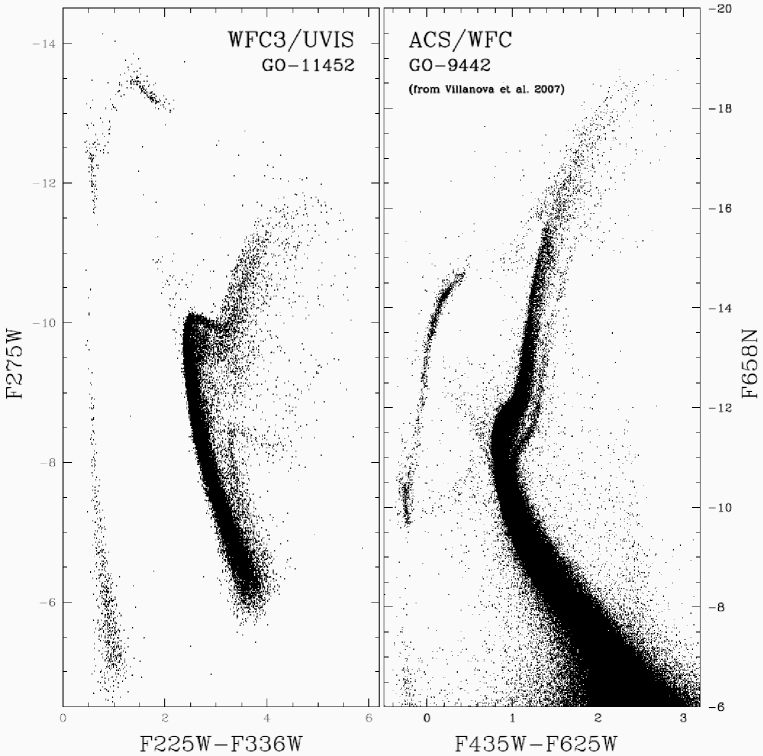
Figure 1: Left: Preliminary color-magnitude diagram of the bright stars in the new WFC3/UVIS data set (fluxes are neither pixel-area- nor L-flat-corrected). Right: Color-magnitude diagram of the stars in our ACS/WFC master frame (from Villanova et al. 2007). Both plots are in instrumental magnitudes.

Figure 2: Left: Color-magnitude diagrams of the high S/N stars in common with the ACS/WFC master frame (F435W), actually used to derive the geometric distortion correction, for each of the WFC3/UVIS filters (F225W, F275W, and F336W).

2 The Geometric Distortion Solutions

The most straightforward way to solve for the GD would be to observe a field where there is a priori knowledge of the positions of all the stars in a distortion-free reference frame. [A distortion-free reference frame is a system that can be transformed into any other distortion-free frame by means of conformal transformations.] Geometric distortion would then show itself immediately as the residuals between the observed relative positions of stars and the ones predicted by the distortion-free frame (on the basis of a conformal transformation).

Thankfully, we possess such an “astrometric flat-field”, moreover with the right magnitude interval, source density, and accuracy. This reference frame is the mosaic of 3$\times$3 Wide Field Channel (WFC) of the Advanced Camera for Surveys (ACS) fields collected – at the end of June 2002– under the program GO-9442 (PI: Cool) reduced by Jay Anderson and published in Villanova et al. (2007). This reference frame was obtained from a total of 18 short and 90 long ACS/WFC exposures in the filters: F435W, F625W, and F658N (see Villanova et al. 2007 for details). The entire field covers an area of 10$\times$10 arcmin², and can be considered distortion-free at the $\sim$0.5 mas level. The catalog contains more than 2 million sources, and we will refer to it as master frame, and to the coordinates of each $i$-source in it with the notation ($X^{\rm master}_{i}$,$Y^{\rm master}_{i}$). A color-magnitude diagram for the stars in the master frame is shown on the right panel of Figure 1.

To derive the WFC3/UVIS GD corrections we closely follow the procedures described in Anderson & King (2003, hereafter AK03) used to correct the GD for each of the four detectors of WFPC2. We represent our solution with a third-order polynomial, which is able to provide our final GD correction to the $\sim$0.025 pixel level in each coordinate ($\sim$1 mas). Higher orders proved to be unnecessary.

Having a separate solution for each chip, rather than one that uses a common center of the distortion in the FoV, allows a better handle of potential individual detector effects (such as a different relative tilt of the chip surfaces, relative motions, etc.). We adopted as the center of our solution, for each chip, the point $(x_{\circ},y_{\circ})_{k=1,2}=(2048,1025)$ [in the raw pixel coordinates, to which we will refer hereafter as ($x,y$)].

For each $i$-star of the master list, in each $k$-chip of each $j$-MEF-file, the distortion corrected position ($x^{\rm corr},y^{\rm corr}$) is the observed position $(x,y)$ plus the distortion correction $(\delta x,\delta y)$:

$$\left\{\begin{array}[]{c}\displaystyle x_{i,j,k}^{\rm corr}=x_{i,j,k}+\delta x_{i,j,k}(\tilde{x}_{i,j,k},\tilde{y}_{i,j,k})\\ \displaystyle y_{i,j,k}^{\rm corr}=y_{i,j,k}+\delta y_{i,j,k}(\tilde{x}_{i,j,k},\tilde{y}_{i,j,k}),\\ \end{array}\right.$$

where $\tilde{x}_{i,j,k}$ and $\tilde{y}_{i,j,k}$ are the normalized positions, defined as:

$$\left\{\begin{array}[]{c}\displaystyle\tilde{x}_{i,j,k}=\frac{x_{i,j,k}-(x_{\circ})_{k}}{(x_{\circ})_{k}}\\ \displaystyle\tilde{y}_{i,j,k}=\frac{y_{i,j,k}-(y_{\circ})_{k}}{(y_{\circ})_{k}}.\\ \end{array}\right.$$

Normalized positions make it easier to recognize the magnitude of the contribution given by each solution term, and their numerical round-off.

The final GD correction for each star, in each chip/image, is given by these two third-order polynomials (we omitted here $i,j,k$ indexes for simplicity):

$$\left\{\begin{array}[]{rcl}\displaystyle\delta x&\!\!\!=\!\!\!&a_{1}\tilde{x}+a_{2}\tilde{y}+a_{3}\tilde{x}^{2}+a_{4}\tilde{x}\tilde{y}+a_{5}\tilde{y}^{2}+a_{6}\tilde{x}^{3}+a_{7}\tilde{x}^{2}\tilde{y}+a_{8}\tilde{x}\tilde{y}^{2}+a_{9}\tilde{y}^{3}\\ \displaystyle\delta y&\!\!\!=\!\!\!&b_{1}\tilde{x}+b_{2}\tilde{y}+b_{3}\tilde{x}^{2}+b_{4}\tilde{x}\tilde{y}+b_{5}\tilde{y}^{2}+b_{6}\tilde{x}^{3}+b_{7}\tilde{x}^{2}\tilde{y}+b_{8}\tilde{x}\tilde{y}^{2}+b_{9}\tilde{y}^{3}.\\ \end{array}\right.$$

Our GD solution is thus fully characterized by 18 coefficients: $a_{1},\dots,a_{9}$, $b_{1},\dots,b_{9}$. However, as done in AK03, we constrained the solution so that, at the center of the chip, it will have its $x$-scale equal to the one at the location $(x_{\circ},y_{\circ})$, and the corrected axis $y^{\rm corr}$ has to be aligned with its $y$-axis at the location $(x_{\circ},y_{\circ})$. This is obtained by imposing $a_{1,k}=0$ and $a_{2,k}=0$. Since the detector axes do not necessarily have the same scales nor are perpendicular to each other, $b_{1,k}$ and $b_{2,k}$ must be free to assume whatever values fit best. Therefore, we have to compute in fact only 16 coefficients (for each chip) to derive our GD solution.

Each $i$-star in the master frame is conformally transformed into each $k$-chip/$j$-image, and cross-identified with the closest source. We indicate such transformed positions with $(X_{i}^{\rm master})^{T_{j,k}}$ and $(Y_{i}^{\rm master})^{T_{j,k}}$. Each of such cross-identifications, when available (of course not all the red sources in the master list were available in the WFC3 UV-filters), generates a pair of positional residuals:

$$\left\{\begin{array}[]{rcl}\displaystyle\Delta x_{i,j,k}&\!\!\!=\!\!\!&x_{i,j,k}^{\rm corr}-(X_{i}^{\rm master})^{T_{j,k}}\\ \displaystyle\Delta y_{i,j,k}&\!\!\!=\!\!\!&y_{i,j,k}^{\rm corr}-(Y_{i}^{\rm master})^{T_{j,k}},\\ \end{array}\right.$$

which reflect the residuals in the GD (with the opposite sign), and depend on where the $i$-star fell on the $k/j$-chip/image (plus random deviations due to non-perfect PSF-fitting and photon noise). Note that our calibration process is an iterative procedure, and that necessarily, at the first iteration, we have to impose $(x^{\rm corr},y^{\rm corr})_{i,j,k}$ $=$ $(x,y)_{i,j,k}$. In each chip/image we have typically $\sim$5500 high-signal unsaturated stars in common with the master frame, leading to a total of $\sim$50 000 residual pairs per chip. [A color-magnitude diagram of the stars actually used to compute the GD solution is shown, for each filter, in Fig.2.]

For each chip, these residuals were then collected into a look-up table made up of $37\times 19$ elements, each related to a region of $110\times 110$ pixels. We chose this particular grid setup because it offers the best compromise between the need for an adequate number of grid points to model the GD, and an adequate sampling of each grid element, containing at least 60 pairs of residuals. For each grid element, we computed a set of five 3$\sigma$-clipped quantities: $\overline{x}_{m,n,k}$, $\overline{y}_{m,n,k}$, $\overline{\Delta x}_{m,n,k}$, $\overline{\Delta y}_{m,n,k}$, and $P_{m,n,k}$; where $\overline{x}_{m,n,k}$ and $\overline{y}_{m,n,k}$ are the averaged positions of all the stars within the grid element $(m,n)$ of the $k$-chip, $\overline{\Delta x}_{m,n,k}$ and $\overline{\Delta y}_{m,n,k}$ are the average residuals, and $P_{m,n,k}$ is the number of stars that were used to calculate the previous quantities. These $P_{m,n,k}$ will also serve in associating a weight to the grid cells when we fit the polynomial coefficients.

To obtain the 16 coefficients describing the two polynomials ($a_{q,k}$ with $q=3,\dots,9$, and $b_{q,k}$ with $q=1,\dots,9$), which represent our GD solution in each chip, we perform a linear least-square fit of the $N=m\times n=37\times 19=703$ data points. Thus, for each chip, we can compute the average distortion correction in each cell ( $\overline{\delta x}_{p,k}$, $\overline{\delta y}_{p,k}$ ) with $N$ relations of the form:

$$k=1,2;~{}p=1,\dots,N:~{}\left\{\begin{array}[]{c}\overline{\delta x}_{p,k}=\displaystyle\sum_{q=3}^{9}a_{q,k}t_{q,p,k}\\ \overline{\delta y}_{p,k}=\displaystyle\sum_{q=1}^{9}b_{q,k}t_{q,p,k}\\ \end{array}\right.$$

(where $t_{1,p,k}={\overline{\tilde{x}}}_{p,k}$, $t_{2,k}={\overline{\tilde{y}}}_{p,k}$, …, $t_{9,k}={\overline{\tilde{y}^{3}}}_{p,k}$), and where the 16 unknown quantities — $a_{q,k}$ and $b_{q,k}$ — are our fitting parameters (16 for each chip) .

In order to solve for $a_{q,k}$ and $b_{q,k}$, we formed, for each chip, one $9\times 9$ matrix $\mathcal{M}_{k}$ and two $9\times 1$ column vectors ${\mathcal{V}}_{a,k}$ and ${\mathcal{V}}_{b,k}$:

$$\mathcal{M}_{k}=\displaystyle\left(\begin{array}[]{cccc}\sum_{p}P_{p,k}t_{1,p,k}^{2}&\sum_{p}P_{p,k}t_{1,p,k}t_{2,p,k}&\cdots&\sum_{p}P_{p,k}t_{1,p,k}t_{9,p,k}\\ \sum_{p}P_{p,k}t_{2,p,k}t_{1,p,k}&\sum_{p}P_{p,k}t_{2,p,k}^{2}&\cdots&\sum_{p}P_{p,k}t_{2,p,k}t_{9,p,k}\\ \vdots&\vdots&\ddots&\vdots\\ \sum_{p}P_{p,k}t_{9,p,k}t_{1,p,k}&\sum_{p}P_{p,k}t_{9,p,k}t_{2,p,k}&\cdots&\sum_{p}P_{p}t_{9,p,k}^{2}\\ \end{array}\right);$$

$$\mathcal{V}_{a,k}=\left(\begin{array}[]{c}\sum_{p}P_{p,k}t_{1,p,k}\overline{\Delta x}_{p,k}\\ \sum_{p}P_{p,k}t_{2,,p,k}\overline{\Delta x}_{p,k}\\ \vdots\\ \sum_{p}P_{p,k}t_{9,p,k}\overline{\Delta x}_{p,k}\\ \end{array}\right);\,\,\,\,\,\,\,\,\,\,\,\,\,\,\,\mathcal{V}_{b,k}=\left(\begin{array}[]{c}\sum_{p}P_{p,k}t_{1,p,k}\overline{\Delta y}_{p,k}\\ \sum_{p}P_{p,k}t_{2,p,k}\overline{\Delta y}_{p,k}\\ \vdots\\ \sum_{p}P_{p,k}t_{9,p,k}\overline{\Delta y}_{p,k}\\ \end{array}\right).$$

The solution is given by two $9\times 1$ column vectors $\mathcal{A}_{k}$ and $\mathcal{B}_{k}$, containing the best fitting values for $a_{q,k}$ and $b_{q,k}$, obtained as:

$${\mathcal{A}_{k}}=\left(\begin{array}[]{c}a_{1,k}\\ a_{2,k}\\ \vdots\\ a_{9,k}\\ \end{array}\right)={\mathcal{M}_{k}}^{-1}{\mathcal{V}}_{a,k};\,\,\,\,\,\,\,\,\,\,\,\,\,\,\,{\mathcal{B}_{k}}=\left(\begin{array}[]{c}b_{1,k}\\ b_{2,k}\\ \vdots\\ b_{9,k}\\ \end{array}\right)={\mathcal{M}_{k}}^{-1}{\mathcal{V}}_{b,k}.$$

With the first set of calculated coefficients $a_{q,k}$ and $b_{q,k}$ we computed the corrections $\delta x_{i,j,k}$ and $\delta y_{i,j,k}$ to be applied to each $i$-star of the $k$-chip in each $j$-MEF file, but actually we corrected the positions only by half of the recommended values, to guarantee convergence. With the new improved star positions, we start-over and re-calculated new residuals. The procedure is iterated until the difference in the average correction from one iteration to the following one —for each grid point— became smaller than 0.001 pixels. Convergence was reached after $\sim 100$ iterations. The coefficients of the final GD solutions for the two chips, and for the three different filters, are given in Table 1.

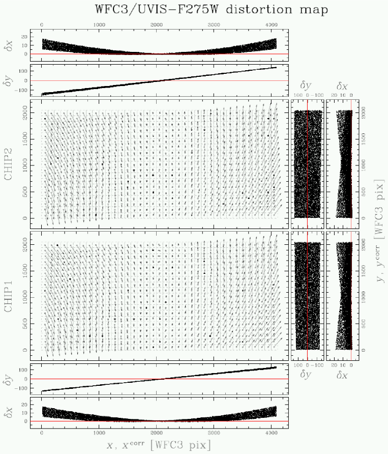
Figure 3: Predicted vs. uncorrected positions. The size of the residual vectors is magnified by a factor of $\times$8 in $x$ and $\times$1.5 in $y$. For each chip we plot also individual residuals as function of $x$ and $y$ axes. Units are expressed WFC3/UVIS pixels in the reference positions ($x_{\circ},y_{\circ}$). For clarity only a random 40% of the residuals is plotted.

In Figure 3 we show for the intermediate filter F275W the total residuals of uncorrected star positions vs. the predicted positions of the master frame, which is representative of our GD solutions. For each chip, we plot the $37\times 19$ cells used to model the GD, each with its distortion vector magnified (by a factor of $\times$8 in $x$, and by a factor of $\times$1.5 in $y$). Residual vectors go from the average position of the stars belonging to each grid cell $(\overline{x},\overline{y})$ to the corrected one $(\overline{x^{\rm corr}},\overline{y^{\rm corr}})$. Side panels show the overall trends of the individual residuals $\delta x$, $\delta y$ along $x$ and $y$ directions (where for clarity we plot only a 40% sub-sample, randomly selected). It immediately strikes the large linear terms in $y$, reaching up to $\sim$140 pixels.

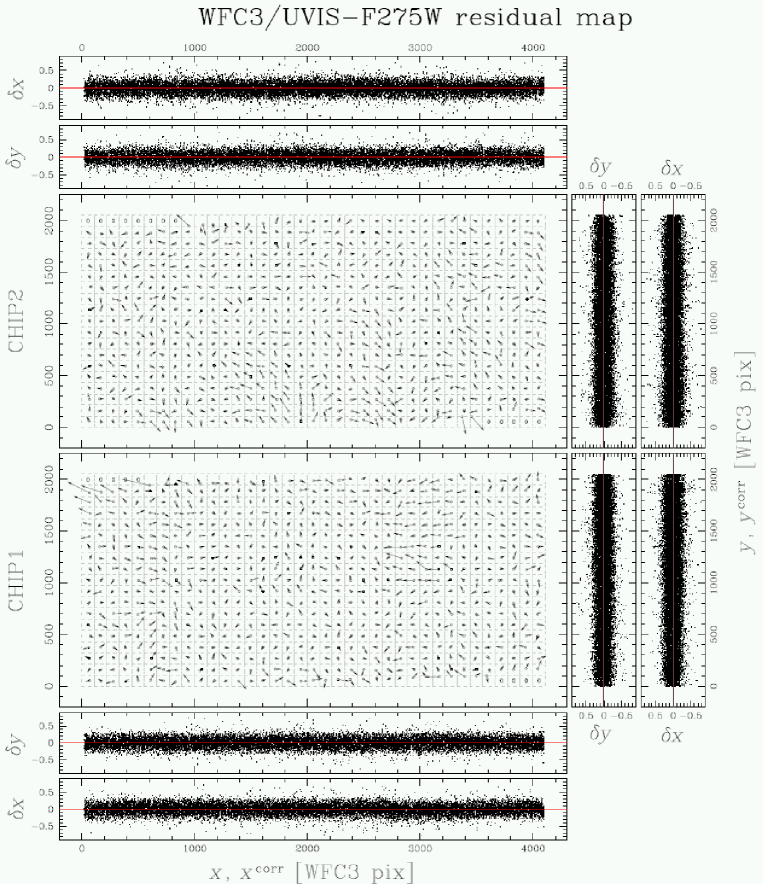
Figure 4: Same as Fig. 3 after the correction was applied. The size of the residuals is now magnified by a factor of 1500.

In Figure 4 we show, in the same way, the remaining residuals after our GD solution is applied. This time we magnified the distortion vectors by a factor $\times$1500 in both axes.

At this point it is very interesting to examine the r.m.s. of these remaining residuals, that show a rather large $\sim$0.15 pixels dispersion. We will see, in the following, that this dispersion can be interpreted as the effect of the internal motions of the cluster stars on the time baseline of $\sim$7 years between the ACS/WFC observations of the reference frame, and the new WFC3/UVIS data set. Indeed, assuming 1) a distance of 4.7 kpc for $\omega$ Cen (van der Marel & Anderson 2009), 2) an internal velocity dispersion of $\sim$18 km s^-1 in our fields (van de Ven et al. 2006), and 3) an isotropic velocity distribution for stars, we would expect to observe in $\sim$7 years a dispersion of the displacements of $\sim$5.5 mas. This dispersion, assuming a pixel scale of $\sim$40 mas for WFC3/UVIS, corresponds to a displacement of $\sim$0.14 pixels (also in good agreement with the recent measurements by Anderson & van der Marel 2009).

To show this more clearly we intercompare the average positions of the nine WFC3/UVIS corrected catalogs in the filter F275W, with those in the F336W, for the stars in common between the two filters. All these images were taken at the same epoch, and so positions of stars are not affected by internal motion effects. The 1-dimension dispersion should reflect our accuracy, and indeed the observed residuals –in this case– have a dispersion of $\sim$0.025 pixels (i.e. $\sim$1 mas). Figure 5 illustrates the two situations. On the left-panel we plot the displacements between the ACS/WFC epoch of the reference frame and the new WFC3/UVIS epoch, while on the right-panel we show the displacements between our corrected position in filter F275W and the corrected positions in F336W. On the left-panel the internal motions of $\omega$ Cen dominate the dispersion, while on the right-panel, there are no internal motions at all, and what we are left with are our errors only.

Unfortunately the WFC3/UVIS images were either not enough, or not well dithered to perform a pure auto-calibration, and we had to use the ACS/WFC reference frame. Nevertheless, even a dispersion of 0.15 pixel within a given cell should be reduced to less than 0.02 pixels if averaged over more than 60 residuals. And this should be regarded as an upper limit, since we are using 703 grid points to constrain 16 parameters.

For this reason, the estimated 0.025 pixel accuracy is larger than we would have expected. We can not exclude that these residuals could be due to a deviation from an isotropic distribution of the internal motion of $\omega$ Cen (i.e. at the level of $\lesssim 3$ km s^-1), or simply by unexpectedly large errors in the adopted ACS/WFC astrometric flat-field (the master frame). Another possibility is that there could be some unexpected (and so far undetected) manufacturing artifact in the WFC3/UVIS detectors which could affect the positions (such as those identified on WFPC2 CCDs, and characterized by Anderson & King 1999, or those of ACS/WFC found by Anderson 2002). Finally, it could simply be a higher frequency spatial variation which can not be properly represented by a polynomial of a reasonable order, but rather by a residual table as done in Anderson (2006) for ACS/WFC. Surely, more data are needed to further improve the GD solutions presented in this work, as well as a better time-baseline for the understanding of its variations. We want to end this section by pointing out that the detection of the internal motions among the stars of a Galactic globular cluster is a rather challenging measurement, and it could well be one of the best demonstrations of the goodness of our derived geometric distortion solutions.

Table 1: The coefficients of the third-order polynomial for each chip and filter.

Term $\!(w)\!\!\!\!\!$	Polyn.	$a_{w,[1]}$	$b_{w,[1]}$	$a_{w,[2]}$	$b_{w,[2]}$
WFC3/UVIS filter F225W
1	$\tilde{x}$	$0.000\!$	$\!129.230\!$	$\!0.000\!$	$\!140.270\!$
2	$\tilde{y}$	$0.000\!$	$\!1.935\!$	$\!0.000\!$	$\!-4.215\!$
3	$\tilde{x}^{2}$	$12.120\!$	$\!0.591\!$	$\!12.021\!$	$\!0.773\!$
4	$\tilde{x}\tilde{y}$	$-6.279\!$	$\!5.553\!$	$\!-6.057\!$	$\!5.496\!$
5	$\tilde{y}^{2}$	$0.064\!$	$\!-3.227\!$	$\!0.001\!$	$\!-3.058\!$
6	$\tilde{x}^{3}$	$0.176\!$	$\!0.029\!$	$\!0.149\!$	$\!0.156\!$
7	$\tilde{x}^{2}\tilde{y}$	$-0.057\!$	$\!0.033\!$	$\!0.022\!$	$\!-0.009\!$
8	$\tilde{x}\tilde{y}^{2}$	$0.004\!$	$\!-0.041\!$	$\!0.061\!$	$\!-0.026\!$
9	$\tilde{y}^{3}$	$0.035\!$	$\!-0.023\!$	$\!0.032\!$	$\!0.028\!$
WFC3/UVIS filter F275W
1	$\tilde{x}$	$0.000\!$	$\!129.270\!$	$\!0.000\!$	$\!140.285\!$
2	$\tilde{y}$	$0.000\!$	$\!1.925\!$	$\!0.000\!$	$\!-4.221\!$
3	$\tilde{x}^{2}$	$12.102\!$	$\!0.581\!$	$\!12.016\!$	$\!0.781\!$
4	$\tilde{x}\tilde{y}$	$-6.284\!$	$\!5.547\!$	$\!-6.040\!$	$\!5.493\!$
5	$\tilde{y}^{2}$	$0.061\!$	$\!-3.241\!$	$\!0.001\!$	$\!-3.048\!$
6	$\tilde{x}^{3}$	$0.178\!$	$\!0.033\!$	$\!0.144\!$	$\!0.163\!$
7	$\tilde{x}^{2}\tilde{y}$	$-0.056\!$	$\!0.054\!$	$\!0.026\!$	$\!0.007\!$
8	$\tilde{x}\tilde{y}^{2}$	$0.005\!$	$\!-0.041\!$	$\!0.051\!$	$\!-0.025\!$
9	$\tilde{y}^{3}$	$0.033\!$	$\!-0.012\!$	$\!0.032\!$	$\!0.020\!$
WFC3/UVIS filter F336W
1	$\tilde{x}$	$0.000\!$	$\!129.438\!$	$\!0.000\!$	$\!140.315\!$
2	$\tilde{y}$	$0.000\!$	$\!1.786\!$	$\!0.000\!$	$\!-4.322\!$
3	$\tilde{x}^{2}$	$12.091\!$	$\!0.676\!$	$\!11.994\!$	$\!0.672\!$
4	$\tilde{x}\tilde{y}$	$-6.188\!$	$\!5.565\!$	$\!-6.135\!$	$\!5.476\!$
5	$\tilde{y}^{2}$	$0.065\!$	$\!-3.155\!$	$\!0.004\!$	$\!-3.152\!$
6	$\tilde{x}^{3}$	$-0.062\!$	$\!0.004\!$	$\!-0.151\!$	$\!0.189\!$
7	$\tilde{x}^{2}\tilde{y}$	$-0.097\!$	$\!0.034\!$	$\!0.074\!$	$\!-0.027\!$
8	$\tilde{x}\tilde{y}^{2}$	$0.016\!$	$\!-0.061\!$	$\!0.040\!$	$\!0.005\!$
9	$\tilde{y}^{3}$	$0.033\!$	$\!0.016\!$	$\!0.033\!$	$\!0.014\!$

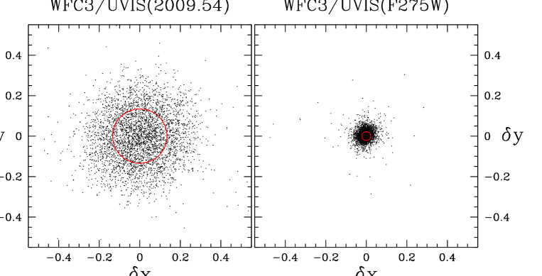
Figure 5: Left: Vector-point diagram of displacements for the stars in common between the ACS/WFC epoch of the master catalog, and the average of the corrected WFC3/UVIS new data in filter F275W. The internal motions of $\omega$ Cen dominate the observed dispersions, but do not prevent a GD solution accurate to $\sim$0.025 WFC3 pixels. Right: Vector-point diagram of displacements for the stars in common between the corrected WFC3/UVIS data in filter F336W, and those corrected for F275W. The images are collected at the same epoch, and no sizable internal motions are present. In this case, the dispersion reflects our errors. The red circles, in both panels, indicate the 1-dimensional dispersion of the residuals, and all quantities are expressed in units of WFC3/UVIS pixels.

Table 2: Interchip transformation parameters. Chip [1] parameters are indicated only for clarity. For chip [2] formal errors are given.

$k$-chip	$\alpha_{[k]}/\alpha_{[1]}$	$\theta_{[k]}$$-$$\theta_{[1]}$	$(x_{\circ}^{[k]})^{\rm corr}_{[1]}$	$(y_{\circ}^{[k]})^{\rm corr}_{[1]}$
	$[$number$]$	$[^{\circ}]$	$[$pixel$]$	$[$pixel$]$
$[1]$	1.00000	0.0000	2048.00	1025.00
$[2]$	1.00595	0.0654	2046.00	3098.34
	$\pm$2/$100\,000$	$\pm$0.001	$\pm$0.03	$\pm$0.03

3 Interchip transformations

For many applications it would be useful to transform the GD corrected positions of each chip into a common distortion-free reference frame. We could then, simply conformally transform the corrected positions of chip [k] into the distortion corrected positions of chip [1], using the following relations:

$$\left(\begin{array}[]{c}x^{\rm corr}_{[1]}\\ y^{\rm corr}_{[1]}\\ \end{array}\right)=~{}\frac{\alpha_{[1]}}{\alpha_{[k]}}~{}\left[\begin{array}[]{cc}\cos(\theta_{[1]}-\theta_{[k]})&\sin(\theta_{[1]}-\theta_{[k]})\\ -\sin(\theta_{[1]}-\theta_{[k]})&\cos(\theta_{[1]}-\theta_{[k]})\\ \end{array}\right]\left(\begin{array}[]{c}x_{[k]}^{\rm corr}-2048\\ y_{[k]}^{\rm corr}-1025\\ \end{array}\right)+\left(\begin{array}[]{c}(x_{\circ}^{[k]})^{\rm corr}_{[1]}\\ (y_{\circ}^{[k]})^{\rm corr}_{[1]}\\ \end{array}\right);$$

where —following the formalism in AK03— we indicate the scale factor as as $\alpha_{[k]}$, the orientation angle with $\theta_{[k]}$, and the positions of the center of the chip $(x_{\circ},y_{\circ})$ in the corrected reference system of chip [1] as $(x_{\circ}^{[k]})^{\rm corr}_{[1]}$ and $(y_{\circ}^{[k]})^{\rm corr}_{[1]}$. Of course, for $k=1$, we end up with the identity. The values of the interchip transformation parameters are given in Table 2, and shown for individual images in Figure 6.

Figure 6: Interchip transformation parameters as obtained from individual images. Data points from F225W are indicated with filled-circles, F275W with triangles, and F336W with crosses. The averages are indicated with solid lines, while the dashed-lines give the formal uncertainties.

4 Average Absolute Scale relative to ACS/WFC

The final step is to link, for each filter, the WFC3/UVIS chip [1] to an absolute plate scale in mas. To this purpose we adopt an average plate scale for our ACS/WFC master frame of 49.7248 mas ACS/WFC-pixel^-1 (from van der Marel et al. 2007), and multiplied it by the –measured– scale factor between the WFC3/UVIS chip [1] and the master frame (which is expressed in ACS/WFC pixels). The results for the individual images and the averages for each filter, are shown in Figure 7, while Table 3 gives the average values in mas pixel^-1. We believe that the differences in the relative values for the three filters are significant. The fact that the plate scales correlate with the wavelength suggests that refraction introduced by either the filters, or by the two fused-silica windows of the dewar, could have some role.

Concerning their absolute values, instead, we have to consider that the velocity of HST around the Earth ($\pm$7 km s^-1) causes light aberration which induces plate-scale variations up to 5 parts in $100\,000$ (Cox & Gilliland 2002), and that our master frame (from Villanova et al. 2007) was not corrected for it.

The ACS/WFC plate scale for the Anderson’s (2006, 2007) GD solution –once corrected for the temporal variations of the linear terms– has proved to be stable at a level of accuracy better than these velocity aberration variations (van der Marel et al. 2007). However, since we are not attempting to correct for this effect on our adopted ACS/WFC master frame, we simply limit the accuracy of the here derived WFC3/UVIS plate-scale absolute values to these accuracies, i.e. 12 parts in $100\,000$.

Figure 7: Absolute scales relative to the one adopted for our ACS/WFC master frame expressed in mas. Each panel shows individual images, for different filters. As in the previous figure, the average values are indicated with solid lines, while the dashed-lines give the formal uncertainties. For reference, we show with error-bars the on-orbit maximum systematic errors introduced by the velocity aberration on the plate scale, i.e. for a velocity of $\pm$7 km s^-1. However, since our master frame has not been corrected for scale variation induced by velocity aberration, these values can not be considered more accurate –in absolute sense– than 12 parts in $100\,000$.

Table 3: Average absolute plate scale of WFC3/UVIS in mas pixel^-1. Accuracy is 12 parts in $100\,000$.

$[$mas pixel-1$]$	F225W	F275W	F336W
$\alpha_{[1]}$	39.760	39.764	39.770

5 Conclusions

By using a limited (but best available) number of exposures with large dithers, and an existing ACS/WFC astrometric flat field, we have found a set of third-order correction coefficients to represent the geometric distortion of WFC3/UVIS in three broad-band ultraviolet filters. The solution was derived independently for each of its two CCDs.

The use of these corrections removes the distortion over the entire area of each chip to an average accuracy of $\sim$0.025 pixel (i.e. $\sim$1 mas), the largest systematics being located in the $\sim$200 pixels closest to the boundaries of the detectors (and never exceeding 0.06 pixels). We advise the use of the inner parts of the detectors for high-precision astrometry. The limitation that has prevented us from removing the distortion at an even higher level of accuracy is the lack of enough observations collected at different roll-angles and dithers which could enable us to perform an auto-calibration.

Nevertheless, the comparison of the mid-2002 ACS/WFC positions with the new WFC3 observations corrected with our astrometric solutions are good enough to clearly show the internal motions of $\omega$ Centauri. These proved to be in perfect agreement with the most recent determinations.

We also derived the average absolute scale of the detector with an accuracy limited by the uncertainties in the plate-scale variations induced by the velocity aberration of the telescope motion in the Earth-Sun system.

For the future, more data with a longer time-baseline are needed to better characterize the GD stability of HST WFC3/UVIS detectors in the medium and long term.

References

- (1) Anderson, J., & King, I. R. 1999, PASP, 111, 1095
- (2) Anderson, J. 2002, The 2002 HST Calibration Workshop: Hubble after the Installation of the ACS and the NICMOS Cooling System, 13
- (3) Anderson, J., & King, I. R. 2003, PASP, 115, 113
- (4) Anderson, J. 2006, The 2005 HST Calibration Workshop: Hubble After the Transition to Two-Gyro Mode, 11
- (5) Anderson, J., Bedin, L. R., Piotto, G., Yadav, R. S., & Bellini, A. 2006, A&A, 454, 1029
- (6) Anderson, J. 2007, , Instrument Science Report ACS 2007-08, 12 pages, 8
- (7) Anderson, J., & van der Marel, R. P. 2009, arXiv:0905.0627
- (8) Bedin, L. R., Salaris, M., Piotto, G., Anderson, J., King, I. R., & Cassisi, S. 2009, ApJ, 697, 965
- (9) Cox, C., & Gilliland, R. L. 2002, The 2002 HST Calibration Workshop : Hubble after the Installation of the ACS and the NICMOS Cooling System, 58
- (10) King, I. R., Anderson, J., Cool, A. M., & Piotto, G. 1998, ApJ, 492, L37
- (11) van de Ven, G., van den Bosch, R. C. E., Verolme, E. K., & de Zeeuw, P. T. 2006, A&A, 445, 513
- (12) van der Marel, R. P., Anderson, J., Cox, C., Kozhurina-Platais, V., Lallo, M., & Nelan, E. 2007, Instrument Science Report ACS 2007-07, 22 pages, 7
- (13) van der Marel, R. P., 2003, Instrument Science Report ACS 2003-10, 21 pages, 10
- (14) van der Marel, R. P., & Anderson, J. 2009, arXiv:0905.0638
- (15) Villanova, S., et al. 2007, ApJ, 663, 296