Bounds on probability of transformations between multi-partite pure states

Abstract

For a tripartite pure state of three qubits, it is well known that there are two inequivalent classes of genuine tripartite entanglement, namely the GHZ-class and the W-class. Any two states within the same class can be transformed into each other with stochastic local operations and classical communication (SLOCC) with a non-zero probability. The optimal conversion probability, however, is only known for special cases. Here, we derive new lower and upper bounds for the optimal probability of transformation from a GHZ-state to other states of the GHZ-class. A key idea in the derivation of the upper bounds is to consider the action of the LOCC protocol on a different input state, namely $1/\sqrt{2}[\ket{000}-\ket{111}]$, and demand that the probability of an outcome remains bounded by 1. We also find an upper bound for more general cases by using the constraints of the so-called interference term and 3-tangle. Moreover, we generalize some of our results to the case where each party holds a higher-dimensional system. In particular, we found that the GHZ state generalized to three qutrits, i.e., $\ket{\mathrm{GHZ}_{3}}=1/\sqrt{3}[\ket{000}+\ket{111}+\ket{222}]$, shared among three parties can be transformed to any tripartite 3-qubit pure state with probability 1 via LOCC. Some of our results can also be generalized to the case of a multipartite state shared by more than three parties.

I Introduction

Entanglement is the most peculiar feature that distinguishes quantum physics from classical physics and lies at the heart of quantum information theory. Thus it is important to get a good understanding of entanglement properties of quantum states. These properties are well understood for bipartite pure states. In the standard distant laboratory paradigm, suppose two distant parties, Alice and Bob, shared a bipartite entangled state. They may apply local operations and classical communications (LOCC) to convert it into another partite state. Bennett et al Bennett1996 has answered the question for the rate of LOCC transformation between bipartite pure states. It is quantified by the von Neumman entropy of a reduced density matrix. For the single-copy case, the optimal conversion probabilities are known for any pure state transformation Lo2001 ; Nielsen1999 ; Vidal1999 . For an LOCC transformation protocol, if it can succeed with probability 1, we call it deterministic, if it can only succeed with a nonzero probability smaller than 1, we call it stochastic, or SLOCC (Stochastic Local Operators and Classical Communications). For mixed states, the question of what the optimal rate of transformations is between them is still largely open.

For multipartite states, however, the problem is much more complicated. There exist different types of entanglement and therefore the transformations are rather involved. For the case of tripartite pure three qubit states, a characterization into six different entanglement classes, of which two contain true tripartite entanglement, exists Dur2000 . One is the GHZ class state, which is defined as

$$\ket{\phi_{GHZ}}=\sqrt{K}(c_{\delta}\ket{0}\ket{0}\ket{0}+s_{\delta}e^{i\varphi}\ket{\varphi_{A}}\ket{\varphi_{B}}\ket{\varphi_{C}})$$ (1)

where

$$\ket{\varphi_{A}}= c_{\alpha}\ket{0}+s_{\alpha}\ket{1}$$ (2)

$$\ket{\varphi_{B}}= c_{\beta}\ket{0}+s_{\beta}\ket{1}$$ (3)

$$\ket{\varphi_{C}}= c_{\gamma}\ket{0}+s_{\gamma}\ket{1}$$ (4)

and K=$(1+2c_{\delta}s_{\delta}c_{\alpha}c_{\beta}c_{\gamma}c_{\phi})^{-1}\in[\frac{1}{2},\infty)$, $c_{\delta}=\cos\delta,s_{\delta}=\sin\delta$, the same for $\alpha,\beta,\gamma,\phi$. The range for the parameters are $\delta\in(0,\frac{\pi}{4}]$, $\alpha,\beta,\gamma\in(0,\frac{\pi}{2}]$ and $\varphi\in[0,2\pi)$.

Another is W class state, which is defined as a state that is unitarily equivalent to

$$\ket{\phi}=(\sqrt{c}\ket{0}+\sqrt{d}\ket{1})\ket{00}+\ket{0}(\sqrt{a}\ket{01}+\sqrt{b}\ket{10})$$ (5)

with $c+d+a+b=1$.

A transformation between any two states of the same class is always possible with non-zero probability. However, here comes the key point. The optimal conversion between the states within the same class of genuine tripartite entangled states is not known. Incidentally, a similar characterization into nine different classes exists for four qubits Verstraete2002 . In 2000, the optimal rate of distillation of a GHZ state from any GHZ-class state was found Ac'in2000a . Very recently, a necessary and sufficient condition for deterministically (i.e., with probability 1) transforming multipartite qubit states with Schmidt rank 2 Eisert2001 have been given Turgut2009 .

In this paper, we present new upper and lower bounds for multipartite entanglement transformations. In particular, we focus on transformations among states with the same Schmidt rank Eisert2001 . We put an emphasis on the transformation from a GHZ state to a GHZ-class state.

But our upper bound can also be generalized to general transformations from one GHZ class state to another. And some of the results are derived for the more general case of higher dimensions and more parties. Especially, we find that all tripartite pure three qubit states can be transformed from 3-term GHZ state $\frac{1}{\sqrt{3}}(\ket{000}+\ket{111}+\ket{222})$ with probability 1. This is a new result. Moreover, some of the general theorems for deterministic transformation are also derived.

The paper is structured as follows. In Section II, we derive upper bounds for the transformation of the GHZ-state to any other state in the GHZ-class. The upper bounds are only non-trivial for a subclass of the GHZ-class. Thus Section III and IV use a different approach that results in upper bounds for a wider class of states. More specific, for any GHZ class state which does not have a known way to be transformed from GHZ state with probability 1, we can find a nontrivial upper bound for the probability of this transformation. And our upper bound can also be effective for the transformation from a GHZ class state to a large class of other GHZ class states. Lower bounds for the transformation of higher dimensional GHZ-states distributed among three or more parties to states with the same Schmidt rank are given in Section V.

II Upper Bound for the Conversion from GHZ state to a GHZ class state

In this section, we derive an upper bound for the conversion of the GHZ-state to any other state of the GHZ-class via LOCC. This upper bound will be nontrivial (i.e., smaller than 1) for $\varphi\in(\frac{1}{2}\pi,\frac{3}{2}\pi)$. The transformation under consideration is given by

$$\ket{\mathrm{GHZ}}=\frac{1}{\sqrt{2}}(\ket{000}+\ket{111})$$

$$\stackrel{{\scriptstyle\textrm{LOCC}}}{{\longrightarrow}}\ket{\Psi} =\sqrt{K}(c_{\delta}\ket{0}\ket{0}\ket{0}+s_{\delta}e^{i\varphi}\ket{\varphi_{A}}\ket{\varphi_{B}}\ket{\varphi_{C}}),$$ (6)

with the parameters defined in introduction.

The LOCC operation is represented by Kraus operators $\{O_{i}=A_{i}\otimes B_{i}\otimes C_{i}\}$. In the following we will refer to different Kraus operators of the LOCC protocol as different branches. Furthermore, a branch $O_{i}\ket{\mathrm{GHZ}}=\ket{\Phi}$ is called a success branch if $\ket{\Phi}\propto\ket{\Psi}$, and a failure branch if there exists no LOCC-operation that can transform $\ket{\Phi}$ into $\ket{\Psi}$ with a non-zero probability, if a branch is neither success nor failure, we call it an undecided branch. An optimal protocol only consists of success and failure branches.

For the following analysis we first recall two known results Dur2000 ; Ac'in2000a

Lemma 1.

For a GHZ-class state $\ket{\Psi}$ we have:

1. The Schmidt rank of $\ket{\Psi}$ is 2 Dur2000 . This means that the minimum number of product states necessary to write $\ket{\Psi}$ as a superposition of them is 2:

   $$\ket{\Psi}=\sum_{i=1}^{2}\alpha_{i}\ket{a_{i}b_{i}c_{i}},$$ (7)

   with $\alpha_{i}\in(0,1)$ and $\braket{a_{i}b_{i}c_{i}}{a_{i}b_{i}c_{i}}=1$.

2. This product state decomposition, i.e., the set $\{(\alpha_{1},\ket{a_{1}b_{1}c_{1}}),(\alpha_{2},\ket{a_{2}b_{2}c_{2}})\}$ is unique Ac'in2000 .

This result leads to

Lemma 2.

For a successful LOCC operation within the GHZ-class,

$$\ket{\Psi} =\alpha_{1}\ket{a_{1}b_{1}c_{1}}+\alpha_{2}\ket{a_{2}b_{2}c_{2}}$$

$$\stackrel{{\scriptstyle\textrm{LOCC}}}{{\longrightarrow}}\ket{\Psi^{\prime}} =\alpha^{\prime}_{1}\ket{a^{\prime}_{1}b^{\prime}_{1}c^{\prime}_{1}}+\alpha^{\prime}_{2}\ket{a^{\prime}_{2}b^{\prime}_{2}c^{\prime}_{2}},$$ (8)

described by the operator $O_{1}$, we must either have the mapping

$$O_{1}\ket{a_{1}b_{1}c_{1}} =o_{1}\frac{\alpha^{\prime}_{1}}{\alpha_{1}}\ket{a^{\prime}_{1}b^{\prime}_{1}c^{\prime}_{1}}$$ (9)

$$O_{1}\ket{a_{2}b_{2}c_{2}} =o_{1}\frac{\alpha^{\prime}_{2}}{\alpha_{2}}\ket{a^{\prime}_{2}b^{\prime}_{2}c^{\prime}_{2}}$$ (10)

or

$$O_{1}\ket{a_{1}b_{1}c_{1}} =o_{1}\frac{\alpha^{\prime}_{2}}{\alpha_{1}}\ket{a^{\prime}_{2}b^{\prime}_{2}c^{\prime}_{2}}$$ (11)

$$O_{1}\ket{a_{2}b_{2}c_{2}} =o_{1}\frac{\alpha^{\prime}_{1}}{\alpha_{2}}\ket{a^{\prime}_{1}b^{\prime}_{1}c^{\prime}_{1}}$$ (12)

with some proportionality constant $o_{1}$, which can be chosen to be real. See Figure 1, Figure 2.

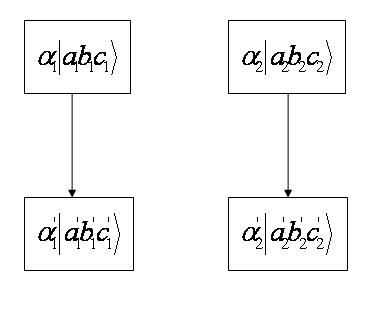
Figure 1: mapping type 1

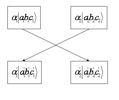
Figure 2: mapping type 2

Proof: Since a LOCC Kraus operator is always of the form $O_{1}=A_{1}\otimes B_{1}\otimes C_{1}$, a product state is always transformed into a product state. With that observation and the fact that the two-term product decomposition of a tripartite GHZ-class state is unique (Lemma 1), Lemma 2 follows. $\Box$

Theorem 1.

An upper bound for the conversion probability for

$$\ket{\mathrm{GHZ}}=\frac{1}{\sqrt{2}}(\ket{000}+\ket{111})$$

$$\rightarrow\ket{\Psi} =\sqrt{K}(c_{\delta}\ket{000}+s_{\delta}e^{i\varphi}\ket{\varphi_{A}\varphi_{B}\varphi_{C}}),$$ (13)

where the parameters are defined in Equation (II), is given by

$$p\leq\min\left\{1,\frac{1+2c_{\delta}s_{\delta}c_{\alpha}c_{\beta}c_{\gamma}c_{\varphi}}{1-2c_{\delta}s_{\delta}c_{\alpha}c_{\beta}c_{\gamma}c_{\varphi}}\right\}$$ (14)

Idea of the Proof: From Lemma 2 we know that, for a success branch, each product state (in the Schmidt term) of the input states have to be mapped to a product state of the output state. This allows us to infer how the same LOCC protocol acts on the phase flipped GHZ state, i.e., $\frac{1}{\sqrt{2}}(\ket{000}-\ket{111})$. From the requirement that the sum of the probabilities for the output states have to sum to 1 for this transformation, we can derive a bound for the parameters arising in the original transformation. This gives a bound on the successful transformation probability.

Proof: Consider the optimal LOCC strategy, given by the Kraus operators $O_{i}=A_{i}\otimes B_{i}\otimes C_{i}$. According to Lemma 2, there are two possibilities to have a successful branch. They are

$$O_{i}\ket{000} =o_{i}c_{\delta}\ket{000}$$ (15)

$$O_{i}\ket{111} =o_{i}e^{i\varphi}s_{\delta}\ket{\varphi_{A}\varphi_{B}\varphi_{C}}$$ (16)

for $i=1,\ldots,n_{1}$, and

$$O_{i}\ket{000} =o_{i}e^{i\varphi}s_{\delta}\ket{\varphi_{A}\varphi_{B}\varphi_{C}}$$ (17)

$$O_{i}\ket{111} =o_{i}c_{\delta}\ket{000}$$ (18)

for $i=n_{1}+1,\ldots,n_{1}+n_{2}$. Both cases give the desired transformation

$$O_{i}\ket{\mathrm{GHZ}}=\frac{1}{\sqrt{2}}o_{i}(c_{\delta}\ket{000}+e^{i\varphi}s_{\delta}\ket{\varphi_{A}\varphi_{B}\varphi_{C}})=\frac{o_{i}}{\sqrt{2K}}\ket{\Psi}$$ (19)

for $i=1,\ldots,n_{1}+n_{2}$. The successful conversion probability is then given by

$$p=\frac{1}{2K}\sum_{i=1}^{n_{1}+n_{2}}o_{i}^{2}.$$ (20)

To get an upper bound for $\sum_{i=1}^{n_{1}+n_{2}}o_{i}^{2}$, we consider how

$$\frac{1}{\sqrt{2}}(\ket{000}-\ket{111})$$ (21)

behaves when put through the Kraus Operator $O_{i}$. We see that

$$O_{i}\frac{1}{\sqrt{2}}(\ket{000}-\ket{111})$$

$$= \frac{1}{\sqrt{2}}o_{i}(c_{\delta}\ket{000}-e^{i\varphi}s_{\delta}\ket{\varphi_{A}\varphi_{B}\varphi_{C}})=\frac{o_{i}}{\sqrt{2K^{\prime}}}\ket{\Psi^{\prime}}$$ (22)

with

$$\ket{\Psi^{\prime}}=\sqrt{K^{\prime}}(c_{\delta}\ket{000}-e^{i\varphi}s_{\delta}\ket{\varphi_{A}\varphi_{B}\varphi_{C}}),\\$$ (23)

where $K^{\prime}=\frac{1}{1-2c_{\delta}s_{\delta}c_{\alpha}c_{\beta}c_{\gamma}c_{\varphi}}$, for $i=1,\ldots,n_{1}+n_{2}$ (up to an overall minus sign for $i=n_{1}+1,\ldots n_{1}+n_{2}$). Thus the conversion probability for this process is given by $\frac{1}{2K^{\prime}}\sum_{i=1}^{n_{1}+n_{2}}o_{i}^{2}$. Being a probability, this has to be bounded by 1, giving $\sum_{i=1}^{n_{1}+n_{2}}o_{i}^{2}\leq 2K^{\prime}$. This together with Equation (20) gives the upper bound

$$p\leq\frac{K^{\prime}}{K}=\frac{1+2c_{\delta}s_{\delta}c_{\alpha}c_{\beta}c_{\gamma}c_{\varphi}}{1-2c_{\delta}s_{\delta}c_{\alpha}c_{\beta}c_{\gamma}c_{\varphi}}$$ (24)

for the process described by Equation (1). $\Box$

Special Case: Regarding the special case, where we have $\ket{\varphi_{A}}=\ket{\varphi_{B}}=\ket{\varphi_{C}}$, $c_{\alpha}=c_{\beta}=c_{\gamma}=\lambda_{a}$, $\varphi=0$, and $c_{\delta}=s_{\delta}=\frac{1}{\sqrt{2}}$, i.e.,

$$\ket{\Psi}=\frac{1}{\sqrt{2}\sqrt{1-\lambda_{a}^{3}}}(\ket{000}-\ket{aaa}),$$ (25)

we get

$$p\leq\frac{1-\lambda_{a}^{3}}{1+\lambda_{a}^{3}}.$$ (26)

Theorem 1 gives a non-trivial upper bound for the transformation from the GHZ-state to a GHZ-class state for all values of $\varphi$ with $\cos\varphi<0$, i.e., $\phi\in(\frac{\pi}{2},\frac{3\pi}{2})$. This nicely shows, that unlike in the bipartite case, where the maximally entangled EPR-state can be tranformed into any other pure two qubit state with probability one, the GHZ-state, which exhibits maximal genuine tripartite entanglement as it maximizes the 3-tangle Coffman2000 and tracing out one qubit results in a totally mixed state, cannot be transformed to all other states in the same class with probability one.

III Failure Branch

Recall in the last section that Eq. (22) gives a trivial bound for the case $\phi\in(\frac{\pi}{2},\frac{3\pi}{2})$. Here, we will derive a useful bound for a larger class of states: we find a upper bound nontrivial for all the cases except $\phi=\frac{\pi}{2}or\frac{3\pi}{2}$ and $\braket{000}{\varphi_{A}\varphi_{B}\varphi_{C}}=0$. In fact, it was shown that these two kinds of transformations can succeed with probability 1 Turgut2009 . Our proof has two important ingredients, namely, the conservation of a new quantity defined as ”interference term” under positive operator valued measures (POVMs) and that the three tangle is an entanglement monotone, which we will discuss in detail in the following.

The idea of our discussion is that, firstly, recall our definition of ”failure branch” as one can not be successful with any nonzero probability, we will prove the weight summation of the so-called interference terms and normalizations of all the branches in an LOCC protocol should be constant during the transformation, which is included in section 3. After that, we find that three tangle is bounded for a fixed interference term which will be defined in this section. Then, we try to see the whole process from the weak measurement aspect, which divides the whole process into many infinitesimal steps and each step changes the state very little. That is to say, the state is changing continuously. Then we stop in the middle and investigate whether there will be a new upper bound. Surprisingly we find there are some new upper bounds and these upper bounds will still be effective in the following steps, even when we reach the end. So it can be used to derive a new upper bound for the supremum success probability of the whole LOCC protocol. Detailed discussion will be showed in section 4.

Theorem 2.

For the transformation from GHZ to GHZ-class state $\ket{\phi}$, failure branches should end with a state with at least one parties’ reduced matrix with rank 1.

Proof: Suppose we would like to get a GHZ-class state $\ket{\phi}=\sqrt{K}(c_{\delta}\ket{0}\ket{0}\ket{0}+s_{\delta}e^{i\varphi}\ket{\varphi_{A}}\ket{\varphi_{B}}\ket{\varphi_{C}})$, where $\ket{0_{A}}$ is linearly independent of $\ket{\varphi_{A}}$, the same for B and C. If there is a state whose reduced density matrices are all of full rank, $\ket{\phi}=\sqrt{K^{\prime}}(c^{\prime}_{\delta}\ket{0}\ket{0}\ket{0}+s^{\prime}_{\delta}e^{i\varphi^{\prime}}\ket{\varphi^{\prime}_{A}}\ket{\varphi^{\prime}_{B}}\ket{\varphi^{\prime}_{C}})$, where $\ket{0_{A}}$ is linearly independent of $\ket{\varphi^{\prime}_{A}}$, the same for B and C. Then it is easy to see, the equation

$$O_{A}\ket{0} =\ket{0}$$ (27)

$$O_{A}\ket{\varphi^{\prime}_{A}} =\ket{\varphi_{A}}$$ (28)

always has a non-trivial solution, the same for B and C. That means we can always transform this state into $\ket{\phi}$ with nonzero probability. $\Box$

III.1 Conservation of interference term

To go further, we want to use the following property of the LOCC Kraus operators. For a complete set of Kraus operators ${O_{i}=A_{i}\otimes B_{i}\otimes C_{i}}$, we have $\sum{O^{+}_{i}O_{i}}=1$.

Suppose that a Kraus operator O satisfies

$$O\ket{000}=\alpha\ket{a_{1}b_{1}c_{1}}$$ (29)

$$O\ket{111}=\beta\ket{a_{2}b_{2}c_{2}}$$ (30)

with $\braket{a_{1}b_{1}c_{1}}{a_{1}b_{1}c_{1}}=\braket{a_{2}b_{2}c_{2}}{a_{2}b_{2}c_{2}}=1$.

Then it can transform $\ket{GHZ}=\frac{1}{\sqrt{2}}(\ket{000}+\ket{111})$ into $\ket{\psi}=\frac{1}{\sqrt{2p}}(\alpha\ket{a_{1}b_{1}c_{1}}+\beta\ket{a_{2}b_{2}c_{2}}$, where $\frac{1}{\sqrt{2p}}$ is the normalization factor and one can check p is exactly the probability of getting $\ket{\psi}$. From here we define interference term and normalization in the following:

Definition 1.

For a normalized GHZ-class state $\ket{\gamma}$ where $\braket{\gamma}{\gamma}=1$, written in the form $\ket{\gamma}=\frac{1}{\sqrt{2}}(\alpha\ket{a_{1}b_{1}c_{1}}+\beta\ket{a_{2}b_{2}c_{2}})$, suppose $\braket{a_{1}b_{1}c_{1}}{a_{2}b_{2}c_{2}}=k$, then we call the real part of $\alpha^{*}\beta k$ the interference term $I$ of $\ket{\gamma}$.

It is easy to see if an operator O transforms $\ket{GHZ}$ to a state $\ket{\psi}$, the interference term of $\ket{\psi}$ is in fact the real part of $\frac{<000|O^{+}O|111>}{p}$, where p is the probability of the branch corresponding to operator O.

Remark 1.

In fact, one can find $I=1-\frac{1}{2}(|\alpha|^{2}+|\beta|^{2})$.

Remark 2.

Note also that $-\infty<I\leq 1$. In other words, it can be unbounded below. This fact will become important in our discussion in Section 4.

Remark 3.

Notice that a failure branch gives a state that is $\mathbf{outside}$ the GHZ class. For such a state, the actual value of interference term depends not only on the state itself, but also on the particular Kraus operator, $O_{i}$, and the initial state, $\phi_{i}$, used to reach the state. So, when we talk about the interference term of failure branches of an SLOCC transformation, we need to be careful: We are not talking about the interference term of the state given by the failure branches, but the interference term determined by the whole transformation protocol.

Theorem 3.

For a complete set of LOCCs which transforms GHZ state to other states, in which the operators are $\{O_{i}\}$, the weighted sum of the interference terms in all the branches should be zero.

$$0=\sum p(O_{i}\ket{GHZ})I(O_{i}\ket{GHZ})$$ (31)

where $p(O_{i}\ket{GHZ})$ is the probability of branch corresponding to the Kraus operator $O_{i}$, and $I(O_{i}\ket{GHZ})$ denotes the interference term I for a state $O_{i}\ket{GHZ}$.

Proof: Suppose the corresponding complete set of Kraus operators consists of ${O_{i}=A_{i}\otimes B_{i}\otimes C_{i}}$. Then we have $\sum{O^{+}_{i}O_{i}}=\mathbbm{1}$. So, we should have

$$0= <000|111>=<000|\mathbbm{1}|111>$$

$$= <000|\sum{O^{+}_{i}O_{i}}|111>$$

$$= \sum{<000|O^{+}_{i}O_{i}|111>}$$

$$= \sum{p(O_{i}\ket{GHZ})\frac{<000|O^{+}_{i}O_{i}|111>}{p(O_{i}\ket{GHZ})}}$$ (32)

From the definition of interference term $I$ we know the real part of the right side of Equation (III.1) is exactly the weighted sum of $I$ of each branch. As the right side of Equation (III.1) is equal to zero, its real part should also be zero, which means for a transformation from $\ket{GHZ}$ to other states, the average value of the interference terms of all the states we get in each branch should be zero. We call this the conservation of interference term. $\Box$

III.2 Conservation of normalization

Definition 2.

For a two-term tripartite state $\ket{\gamma}$, written in the form $\ket{\gamma}=\frac{1}{\sqrt{2}}(\alpha\ket{a_{1}b_{1}c_{1}}+\beta\ket{a_{2}b_{2}c_{2}}$, then we call $\frac{1}{2}(|\alpha|^{2}+|\beta|^{2})$ the normalization of $\ket{\gamma}$.

Easy to see if an operator O transforms $\ket{GHZ}$ to the state $\ket{\psi}$, the normalization of $\ket{\psi}$ is in fact $\frac{<000|O^{+}O|000>+<111|O^{+}O|111>}{2p}$, where p is the probability. And because O is a positive operator, normalization should be always no less than zero.

Suppose the corresponding complete set of Kraus operators consists of $\{O_{i}=$ $A_{i}\otimes B_{i}\otimes C_{i}\}$. Then we have $\sum{O^{+}_{i}O_{i}}=\mathbbm{1}$. So we should have

$$1= <GHZ|GHZ>$$

$$= \frac{1}{2}(<000|+<111|)(|000>+|111>)$$

$$= \frac{1}{2}(\braket{000}{000}+\braket{111}{111})$$

$$= \frac{1}{2}(\sum{\braket{000}{O^{+}_{i}O_{i}}{000}}+\sum{\braket{111}{O^{+}_{i}O_{i}}{111}})$$

$$= \sum{p(O_{i}\ket{GHZ})\frac{<000|O^{+}_{i}O_{i}|000>+<111|O^{+}_{i}O_{i}|111>}{2p(O_{i}\ket{GHZ})}}$$ (33)

From the definition of normalization we know it is exactly the weighed sum of the normalization of each branch. That is to say, for a transformation from $\ket{GHZ}$ to other states, the average value of the normalization of all the states we get in each branch should be 1. And recall that normalization can be no less than zero. So each term in the summation should be no larger than 1, which means for each branch, the product of its probability and the normalization of the state it gets should be no larger than 1.

In fact, the conservation of normalization can be derived from conservation of interference term. However, conservation of the normalization also gives the following. For each branch, the product of its probability and the normalization of the state it gets should be no larger than 1. The fact is also useful in determining the upper bound of transformation probability.

The basic idea is that, if we know the state we want and the state failure branch gives, equations (III.1) and (III.2) combined with the fact that the summation of probability should be one can give us some implication about the supremum success probability. For example, we can have the following theorem:

Theorem 4.

For a transformation protocol from GHZ state to a GHZ-class state $\ket{\phi}$ whose interference term is x, which is positive (negative), if there exists a y (y $>$ 0), such that, the interference term of all the failure branches are larger than -y (smaller than y), we have an upper bound for its successful probability $p_{s}$ in the following:

if $x>0$:

$$p_{s}\leq p^{U}(-y)=\frac{y}{x+y}.$$ (34)

if $x<0$:

$$p_{s}\leq p^{U}(y)=-\frac{y}{x-y}.$$ (35)

See

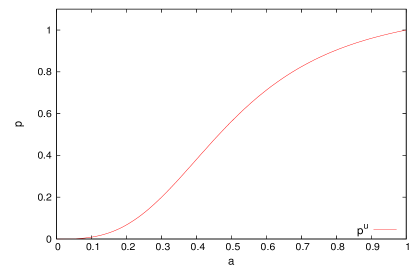
Figure 3: The value of $p^{U}$ as a function of a

In this figure, $a=(\frac{y}{y-1})^{\frac{1}{3}}$. So when a goes from 0 to 1, y goes from 0 to $\infty$. Note that as y goes to infinity, a goes to 1. We express the value as a function of a because it will be easier for us to combine different graphes into one graph later.

Proof: Take $x>0$, suppose there are n failure branches, whose probabilities are $p_{f_{1}},p_{f_{2}},\cdot,p_{f_{n}}$, and the corresponding interference terms are $-y_{1},-y_{2},\cdot-y_{n}$, then we have

$$p_{s}x-\sum p_{f_{i}}y_{i}=0$$ (36)

$$p_{s}+\sum p_{f_{i}}=1$$ (37)

Rewrite it in the following form,

$$p_{s}x-p_{ft}y^{\prime}=0$$ (38)

$$p_{s}+p_{ft}=1$$ (39)

where $p_{ft}=\sum p_{f_{i}}$ and $y^{\prime}=\frac{\sum p_{f_{i}}y_{i}}{p_{ft}}$. The solution of it is

$$p_{s}=\frac{y^{\prime}}{x+y^{\prime}}$$ (40)

As the interference term of all the failure branches are larger than -y, we have $y^{\prime}<y$, then we can get $p_{s}<p^{U}(-y)=\frac{y}{x+y}$. The discussion for the case when $x<0$ is similar. $\Box$

Remark 4.

Recall the range of the I can be $-\infty<I\leq 1$, which means I can be unbounded below. Then in the $x>0$ case, if the I of the failure branch goes to $-\infty$, or we can say y goes to $\infty$, we will have $p^{U}(-y)$ arbitrary close to 1. Therefore, theorem 4 alone is not enough for establishing a non-trivial upper bound. To derive a non-trivial upper bound, we need to find some additional constraints which are related to the interference term. In fact, this is what we will do in section 4.

IV Upper Bound for a general case

In this section, we will find an upper bound in a more general case. Recall the problem of theorem 4 is that the interference can be unbounded below. So we would like to find an additional constraint. It turns out that the fact that the 3-tangle, a measure of tripartite entanglement introduced in Coffman2000 , is an entanglement monotone (i.e., it cannot increase on average under LOCCs) is precisely what we need Dur2000 .

Our strategy is that, for any possible transformation protocol, we would like to construct a new protocol that has the following two properties: 1. It has an upper bound for the maximal successful probability of transformation which is obviously smaller than one; 2. We can reconstruct the original protocol from this new protocol, which means the successful probability of this new protocol can be no less than the original one. The way we construct such a protocol is given in 4.2 and the bound of it will be given in 4.3, in which we deal with a special example: the transformation from GHZ state to a special GHZ class state $\ket{\phi}=\gamma(\ket{000}+\ket{aaa})$. In 4.4, we will generalize this bound to more general cases, where we find for any transformation from one GHZ-class state $\ket{\phi}$ to another GHZ-class state $\ket{\psi}$ with different interference terms, we can find an nontrivial upper bound for the successful probability.

IV.1 interference term and the maximal value of the 3-tangle of a GHZ-class state

Now consider such a question: Suppose we have an unknown GHZ class state $\ket{\phi_{GHZ}}=\sqrt{K}(c_{\delta}\ket{0}\ket{0}\ket{0}+s_{\delta}e^{i\varphi}\ket{\varphi_{A}}\ket{\varphi_{B}}\ket{\varphi_{C}})$ with a given interference term f, what is the maximal value of the 3-tangle $\tau_{ABC}$ Dur2000 ?

Theorem 5.

For a GHZ class $\ket{\phi_{GHZ}}$, if its interference term is I, then the maximal value of its 3-tangle is $\frac{(1-a^{2})^{3}}{(1+a^{3})^{2}}$, where a = $(\frac{f}{1-f})^{\frac{1}{3}}$.

The proof will be given in the appendix.

IV.2 ”stop and reconstruct” procedure

From Oreshkov2005 , we know every measurement can be seen as constructed by many infinitesimal steps of weak measurement, that is, a measurement which only slightly changes the original state. From this view, to get a better understanding of the transformation protocol, we would like to try to reduce the case where a failure branch gives an $I>I_{0}$ (some prescribed value) to the case where an undecided branch has $I=I_{0}$. That is to say, we are using a reduction idea. First we need to answer the following question: Can we stop at some intermediate point and reconstruct the original measurement? It turns out that the answer is yes. In fact, from Oreshkov2005 , the following theorem follows easily.

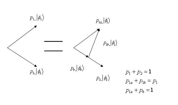
Figure 4: ”stop and reconstruct” for a two-outcome measurement

Theorem 6.

A two-outcome measurement $\{M_{1},M_{2}\}$ can be reconstructed by stopping at an immediate step $\{\sqrt{1-e^{-2x}}M^{\prime}_{1},\sqrt{1+e^{-2x}}M^{\prime}(x)\}$ and a reconstructing measurement ${\{M^{\prime}(x,+\infty),M^{\prime}(x,-\infty)\}}$, where $M^{\prime}_{1}=\sqrt{M^{+}_{1}M_{1}}$ and

$$M^{\prime}(x,+\infty)= \sqrt{\frac{1+\tanh(x)}{I+\tanh(x)(M^{\prime 2}_{2}-M^{\prime 2}_{1})}}M^{\prime}_{2},$$ (41)

$$M^{\prime}(x,-\infty)= \sqrt{\frac{1-\tanh(x)}{I+\tanh(x)(M^{\prime 2}_{2}-M^{\prime 2}_{1})}}M^{\prime}_{1}$$ (42)

See Figure 4 for a graphic discription.

Proof: Firstly, from polar decomposition we have $M_{1}=U_{1}M^{\prime}_{1},M_{2}=U_{2}M^{\prime}_{2}$, where $U_{1}$ and $U_{2}$ are unitary, $M^{\prime}_{2}=\sqrt{M^{+}_{2}M_{2}}$. Then $\{M^{\prime}_{1},M^{\prime}_{2}\}$ is also a measurement. As $M^{\prime}_{1}$ and $M^{\prime}_{2}$ are positive, it can be reconstructed from infinitesimal steps .Oreshkov2005 Secondly, instead of measure $\{M^{\prime}_{1},M^{\prime}_{2}\}$, we stop at $M^{\prime}(x)=\sqrt{\frac{I+\tanh(x)(M^{\prime 2}_{2}-M^{\prime 2}_{1})}{2}}$ before we reach $M^{\prime}_{2}$, that is to say, we perform measurement $\{\sqrt{1-e^{-2x}}M^{\prime}_{1},\sqrt{1+e^{-2x}}M^{\prime}(x)\}$. The effect is we still got $M^{\prime}_{1}\rho M^{\prime+}_{1}/p_{1}$ but the probability become $\sqrt{1-e^{-2x}}p_{1}$, but instead of get $M^{\prime}_{2}\rho M^{\prime+}_{2}/p_{2}$, we get $M^{\prime}(x)\rho M^{\prime+}(x)/p(x)$ where $p(x)=Tr(M^{\prime}(x)\rho M^{\prime+}(x))$. Thirdly, we do nothing to the $M^{\prime}_{1}$ branch, but do a POVM ${\{M^{\prime}(x,+\infty),M^{\prime}(x,-\infty)\}}$.

On the M’(x) branch, it is easy to prove that,

$$M^{\prime}(x,\infty)M^{\prime}(x)=e^{-x}M^{\prime}_{1},M^{\prime}(x,-\infty)M^{\prime}(x)=M^{\prime}_{2},$$ (43)

So in total, we perform a POVM $\{\sqrt{1-e^{-2x}}M^{\prime}_{1},e^{-x}M^{\prime}_{1},M^{\prime}_{2}\}$, that is just the same as $\{M^{\prime}_{1},M^{\prime}_{2}\}$. Finally, if we get the result of measurement $M^{\prime}_{1}(M^{\prime}_{2})$, perform a unitary transformation $U_{1}(U_{2})$, we can reconstruct $\{M_{1},M_{2}\}$ with a stop in the middle. QED.

However, a protocol may contain many measurements and measurements with more than two outcomes, can we still use this method to stop in the middle and reconstruct everything?

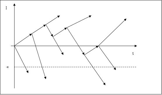
Figure 5: The original protocol written in the many two-outcome measurements form

The answer is yes. To show this, first we need to rewrite every measurement in the protocol into a sequence of two-outcome measurements Andersson2007 , see Figure 5. Then the protocol consists of only two-outcome measurements. So the ”stop and reconstruct” can work for each of them. The only thing is that, now, each two-outcome measurement may be related to many other two-outcome measurements, so during the ”stop and reconstruct” process, many measurements might be affected. How can we be sure we can reconstruct everything? For this problem, notice that these two-outcome measurements are all in order. Then when we do the ”stop and reconstruct”, the principle is that we should always stop at the earlier two-outcome measurement first. Moreover, we need to reconstruct the earlier ones first. See Figure 6.

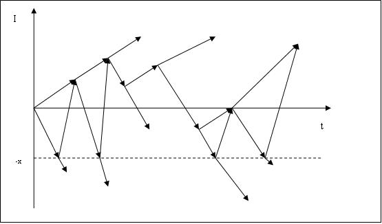
Figure 6: ”stop and reconstruct” for general protocol, I stands for the interference term

IV.3 Example: $\ket{GHZ}\rightarrow\ket{\phi}=\gamma(\ket{000}+\ket{aaa})$

Now, we want to find an upper bound for the success probability of the transformation.

Theorem 7.

Suppose we have a SLOCC transformation protocol from $\ket{GHZ}$ to $\ket{\phi}=\gamma(\ket{000}+\ket{aaa})$, where $\ket{a}=c\ket{0}+\sqrt{1-c^{2}}\ket{1}$ and $c\in(0,1]$. Suppose the successful probability is $p_{m}$. Then we can always find a protocol consisting of only successful and failure branches which has a successful probability no less than $p_{m}$.

Proof: If the protocol is in that form, we do nothing. If the protocol has some branches which are neither successful nor failure. Then we do nothing to the successful or failure branches. However, for the undecided branches, from the definition of it we know we can always find a POVM that can transform it into the desired state with nonzero probability $\delta_{p}$. Then the total successful probability is $p_{m}+\delta_{p}$, which is higher than $p_{m}$. In all, we can always find a protocol consisting of only successful and failure branches which have a successful probability no less than $p_{m}$. QED.

Now modify the protocol we get in the first step in the following way:

Suppose we can find at least one failure branch that have interference term smaller than -y, where ${y\geq 0}$. then we can find a x, where ${0\leq x\leq y}$. As our initial interference term is zero, now we can use the weak measurement idea to let all the branches stop if its interference term reaches -x and do nothing to the branches which never reach -x. And we can get a new protocol in Figure 7

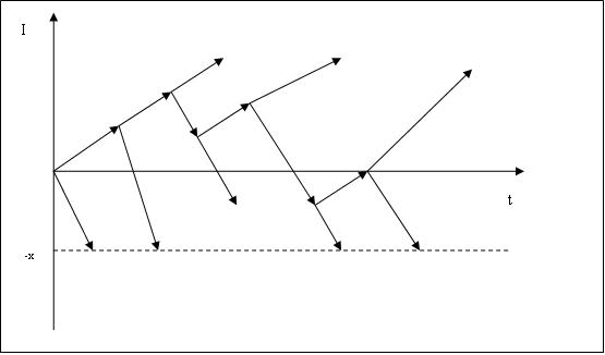
Figure 7: The new protocol, which can reconstruct the original one

Remark 5.

Note that to make this new protocol work, we have applied the intermediate value theorem. That is to say, we implicitly assume that the interference terms, I, of the two intermediate states specified in Theorem 5, are continuous functions of x. This assumption works because, from Oreshkov2005 , we know $M(x,\delta x)$ changes the state given by $M(x)\ket{GHZ}$ very little, or we can say it is a weak measurement. While from the expression of interference term Equation (91) in Appendix, we know interference term is a continuous function of the parameters of the state. Then, as the state changes very little under the weak measurement, the interference term also changes continuously.

Then we get a new protocol. It has two properties:

1) There are three kinds of branches: failure branches with interference term larger than or equal to -x, successful branches and the branches neither successful nor failure with interference term -x.

2) From the ”stop and reconstruct” part, we know we can reconstruct the original protocol by performing LOCCs (may be a sequence of measurements) just on these branches which have interference term -x and do nothing on other branches. That is to say, just do LOCCs on the -x branches, we can get a total successful probability no less than the original one. So, if we have an upper bound of successful probability for the new protocol, that should also be an upper bound for the original one.

Then we can find the upper bound for this new protocol. Now, the protocol consists of three kinds of branches: successful branches, failure branches with interference term larger than or equal to -x, and undecided branches with interference term -x. The total successful probability of this protocol consists of two probability: the already existing successful branches’ total probability $p_{se}$ and the probability we can transform from the -x branches to the states we want.

Theorem 8.

As in Theorem 7, we consider a SLOCC transformation from $\ket{GHZ}$ to $\ket{\phi}=\gamma(\ket{000}+\ket{aaa})$. For all the possible new protocols shown in Figure 7, there is an upper bound for the success probability

$$\bar{p_{s}}(-x)=p_{as}(-x)+p_{u}(-x)*p_{m}(s|-x)$$ (44)

where $p_{as}(-x)$ is the already successful branches in this condition, while $p_{u}(-x)$ is the probability of the undecided branches with interference term -x. And $p_{m}(s|-x)$ is the maximal probability to transform a GHZ-class state with interference term -x into the destination state $\phi_{s}$. And we will get

$p_{as}=\frac{\frac{a^{3}}{1-a^{3}}}{\frac{c^{3}}{1+c^{3}}+\frac{a^{3}}{1-a^{3}}}$, $p_{u}(-x)=1-p_{as}$,

$p_{m}(s|-x)=min(\frac{max(\tau_{ABC}(\phi|I(\phi)=-x))}{\tau_{ABC}(\phi_{s})},1)$

where a is the solution of the equation $x=\frac{a^{3}}{1-a^{3}}$, $\tau_{ABC}$ stands for the 3-tangle.

We firstly consider the case that there exists no failure branches with interference term larger than -x, later we will show the other case can only give an upper bound smaller than in this case.

Lemma 3.

If the new protocol shown in Figure 7 consists of only successful branches and branches with interference term -x (no failure branches with interference term larger than -x), it has an upper bound

$$\bar{p_{s}}(-x)=p_{as}(-x)+p_{u}(-x)*p_{m}(s|-x)$$ (45)

where the parameters are defined in Theorem 8.

Proof: For the already existing successful branches, the total probability is determined by -x and the conservation of interference term. As $x=\frac{a^{3}}{1-a^{3}}$, we have

$$p_{as}(-x)I(\ket{\phi_{s}})-p_{u}(-x)x=0$$ (46)

$$p_{as}(-x)+p_{u}(-x)=1$$ (47)

Solving Eqs. (66) and (67), we can find $p_{as}(-x)=\frac{\frac{a^{3}}{1-a^{3}}}{\frac{c^{3}}{1+c^{3}}+\frac{a^{3}}{1-a^{3}}}$.

For the maximum value of $p_{s}(-x)$, using the 3-tangle idea, we know it is bounded by $p_{u}(-x)*p_{m}(s|-x)$ where

$$p_{m}(s|-x)=min(\frac{max(\tau_{ABC}(\phi|I(\phi)=-x))}{\tau_{ABC}(\phi_{s})},1)$$ (48)

Then we find an upper bound for the successful probability of this new protocol when there is no failure branch having interference term larger than -x:

$$\bar{p_{s}}(-x)=p_{as}(-x)+p_{u}(-x)*p_{m}(s|-x)$$ (49)

$\Box$

Remark 6.

To show it is really an upper bound for the successful probability for the new protocol, we need to show if there is any other failure branch with interference term larger than -x, we can only get a successful probability smaller than this.

Proof of Theorem 8: To prove this theorem, we just need to prove the following: If the new protocol contains a failure branch which has an interference term larger than -x, it has an upper bound for the success probability smaller than what we get in Lemma 3.

Consider the conservation of interference term, now we have:

$$p^{\prime}_{as}(-x)I(\ket{\phi_{s}})+\sum p_{fi}I(\ket{\phi_{f_{i}}})-p^{\prime}_{u}(-x)x=0$$ (50)

$$p^{\prime}_{as}(-x)+\sum p_{fi}+p^{\prime}_{u}(-x)=1$$ (51)

which can be rewritten as from Corollary 2

$$p^{\prime}_{as}(-x)I(\ket{\phi_{s}})-p"(-x^{\prime})x^{\prime}=0$$ (52)

$$p^{\prime}_{as}(-x)+p"(-x^{\prime})=1$$ (53)

where

$$x^{\prime}=\frac{\sum p_{fi}I(\ket{\phi_{f_{i}}})-p^{\prime}_{u}(-x)x}{\sum p_{fi}+p^{\prime}_{u}(-x)}$$ (54)

$$p"(-x^{\prime})=\sum p_{fi}+p^{\prime}_{u}(-x)$$ (55)

As $I(\ket{\phi_{f_{i}}})>-x$, we know $-x^{\prime}>-x$, so $p^{\prime}_{as}(-x)<p_{as}(-x)$. Let the difference between $p^{\prime}_{as}(-x)$ and $p_{as}(-x)$ be $\delta_{s}$, then we have $\delta_{s}=p_{as}(-x)-p^{\prime}_{as}(-x)$, so $\delta_{s}>0$ and $p"(-x^{\prime})=p_{u}(-x)+\delta_{s}$. As $\sum p_{fi}>0$, we have $p^{\prime}(-x)<p"(-x^{\prime})=p_{u}(-x)+\delta_{s}$. So the total successful probability in this case is

$$\bar{p^{\prime}_{s}}=p^{\prime}_{as}(-x)+p^{\prime}(-x)*p(s|-x)$$

$$\leq p^{\prime}_{as}(-x)+p^{\prime}(-x)*p_{m}(s|-x)$$

$$< p_{as}(-x)-\delta_{s}+(p_{u}(-x)+\delta_{s})*p_{m}(s|-x)$$

$$< p_{as}(-x)+p_{u}(-x)*p_{m}(s|-x)$$

$$+\delta_{s}(p_{m}(s|-x)-1)$$

$$\leq p_{as}(-x)+p_{u}(-x)*p_{m}(s|-x)$$

$$= \bar{p_{s}}(-x)$$ (56)

Here, in the second last step, we have used the fact that $p_{m}(s|-x)$ can not be larger than one. So we know it is really an upper bound for the successful probability for the new protocol, which should also be an upper bound for the successful probability for the original protocol, and an upper bound for the transformation protocols which contains at least on failure branch which has interference term smaller than -x ( or we can say it passes -x). So we have $\bar{p^{\prime}_{s}}<\bar{p_{s}}(-x)$, which means $\bar{p_{s}}(-x)$ is an upper bound for the new protocol. $\Box$

Corollary 1.

As in Theorem 7, we consider a SLOCC transformation from $\ket{GHZ}$ to $\ket{\phi}=\gamma(\ket{000}+\ket{aaa})$. If a protocol contains at least one failure branch whose interference term is smaller than -y, its successful probability should be bounded by all the $\bar{p_{s}}(-x)$, where $0\leq x\leq y$.

Proof: If we see every branch from the weak measurement idea. We will find the interference term should change continuously, so we can stop at any point between 0 and -y. For each point we choose, we can get an upper bound. And all the upper bounds should be the upper bounds of the original branch. $\Box$

Corollary 2.

For a LOCC transformation protocol from $\ket{GHZ}$ to $\ket{\phi}=\gamma(\ket{000}+\ket{aaa})$, if the minimum interference term of all the failure branches is -z, then its successful probability should be bounded by

$$p_{bound}(-z)=\min(p^{U}(-z),\bar{p}_{\tau_{ABC}}(-z))$$ (57)

where $\quad\bar{p}_{\tau_{ABC}}(-z))=\min_{0\leq x\leq z}(\bar{p_{s}}(-x))$.

Proof: If the minimum interference term is -z, then from Theorem 4, we know there is an upper bound $p^{U}(-z)=\frac{z}{I(\ket{\phi_{s}})+z}$, which is in fact $p_{as}(-z)$. As it is bounded by all the $\bar{p_{s}}(-x)$, where $0\leq x\leq z$, we can find another upper bound $\bar{p}_{\tau_{ABC}}(-z))=\min_{0\leq x\leq z}(\bar{p_{s}}(-x))$. See Figure 8 for the relation between $\bar{p_{s}}$ and $\bar{p}_{\tau_{ABC}}$. Then the minimum of these two bounds is also an upper bound, which we call $p_{bound}(-z)$.

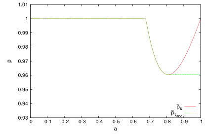
Figure 8: the relation between $\bar{p_{s}}$ and $\bar{p}_{\tau_{ABC}}$

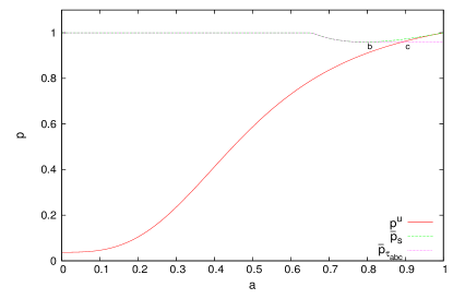
Figure 9: The upper bound for the transformation

In this figure, $a=(-\frac{x}{x-1})^{\frac{1}{3}}$. So when a goes from 0 to 1, x goes from 0 to $\infty$. The dashed line is the plot of $\bar{p_{s}}$ as a function of -x, the dot line is the plot of $\bar{p}_{\tau_{ABC}}$, the solid line is the plot of $p^{U}$. Notice that point b corresponds to the minimum value of $\bar{p_{s}}$, before b, $\bar{p_{s}}$ decreases monotonically. So before b, $\bar{p}_{\tau_{ABC}}$ is the same as $\bar{p_{s}}$, while after b, $\bar{p}_{\tau_{ABC}}$ remains to be the value of $\bar{p_{s}}$ at b. Another thing is that before c, $p^{U}$ is smaller than $\bar{p}_{\tau_{ABC}}$, while after c, $\bar{p}_{\tau_{ABC}}$ is smaller than $p^{U}$. So the final plot we get for the upper bound is the solid line before c and the dot line after c, which we call upper bound line. The meaning of this upper bound line is that, for a given transformation protocol, if the smallest interference term of all the failure branches is -y, let $k=(-\frac{y}{y-1})^{\frac{1}{3}}$, the success probability can not be larger than the corresponding point in the upper bound line. Consider all of the possible protocols (a goes from 0 to 1), the upper bound of the transformation probability is the largest value of the points on the upper bound line, which is just the minimum value of $\bar{p_{s}}$

Theorem 9.

An upper bound of LOCC transformation from GHZ state to a specific GHZ class state $\ket{\phi}=\gamma(\ket{000}+\ket{aaa})$ is the maximum value of $p_{bound}(-z)$ where $z\in[0,+\infty)$. And it is in fact the minimum value of $\bar{p_{s}}(-z)$, where $z\in[0,+\infty)$.

Proof: The basic picture of our proof can be represented in Figure 9.

Now we consider all the possible transformation protocols. Then the value of the minimum interference term -z may vary from 0 to $\infty$. (We can always find a protocol giving a very small value of -z, while its successful probability is still bounded.) Easy to see an upper bound is the maximum value of $p_{bound}(-z)$ for all the possible values of z, where $z\in[0,\infty)$. In fact, we can find the upper bound we get for this transformation is the minimum value of $\bar{p_{s}}(-z)$, where $z\in[0,+\infty)$. $\Box$

Put $\tau_{ABC}(\phi)=\frac{(1-c^{2})^{3}}{(1+c^{3})^{2}}$, in to the equation, we can get the upper bound. The analytic value is hard to get, if we put c=0.5. The minimum value of $\bar{p_{s}}(-x)=p_{as}(-x)+p_{u}(-x)*p_{m}(s|-x)$ is 0.9604 at x=1.13062, which is less than 1.

IV.4 general case

In the above, we have considered an upper bound for the special case of $\ket{GHZ}\rightarrow\ket{\phi}=\gamma(\ket{000}+\ket{aaa})$ to find the upper bound for it. Now, we will consider two more general cases. First, we will consider the transformation $\ket{GHZ}\rightarrow\ket{\phi_{GHZ}}=\sqrt{K}(c_{\delta}\ket{0}\ket{0}\ket{0}+s_{\delta}e^{i\varphi}\ket{\varphi_{A}}\ket{\varphi_{B}}\ket{\varphi_{C}})$, which is the general GHZ class state; Second, we will consider a general GHZ class state to another general GHZ class state.

1. $\ket{GHZ}\rightarrow\ket{\phi_{GHZ}}=\sqrt{K}(c_{\delta}\ket{0}\ket{0}\ket{0}+s_{\delta}e^{i\varphi}\ket{\varphi_{A}}\ket{\varphi_{B}}\ket{\varphi_{C}})$. In this case, we just need to change the expression for the interference term and 3-tangle of the destination state into

$$Interference\;term:I(\phi_{s})=\frac{2c_{\alpha}c_{\beta}c_{\gamma}s_{\delta}c_{\delta}c_{\varphi}}{(1+2c_{\alpha}c_{\beta}c_{\gamma}s_{\delta}c_{\delta})}$$ (58)

$$3-tangle:\tau_{ABC}(\phi_{s})=\frac{4s^{2}_{\alpha}s^{2}_{\beta}s^{2}_{\gamma}s^{2}_{\delta}c^{2}_{\delta}}{(1+2c_{\alpha}c_{\beta}c_{\gamma}s_{\delta}c_{\delta})^{2}}$$ (59)

Then we can use the similar process, except changing the corresponding value of Interference term and 3-tangle, see the following for details.

Firstly, using the ”stop and reconstruct” method to get the new protocol with only successful branches and undecided branches with interference term x. We have

$$p_{as}(x)I(\ket{\phi_{s}})+p_{u}(x)x =0$$ (60)

$$p_{as}(x)+p_{u}(x) =1$$ (61)

We have

$$p_{as}(x) =\frac{x}{x-I(\ket{\phi_{s}})}=1-p_{u}(x)$$ (62)

$$p_{m}(s|x) =\min(\frac{max(\tau_{ABC}(\phi|I(\phi)=x))}{\tau_{ABC}(\phi_{s})},1)$$ (63)

Then, the supremum success probability of this new protocol should be bounded by

$$\bar{p_{s}}(x)=p_{as}(x)+p_{u}(x)*p_{m}(s|x)$$ (64)

Consider all possible protocols, we find the minimum of $\bar{p_{s}}(x)$ where $x\in[0,\frac{1}{2}]$ if $I(\ket{\phi_{s}})<0$ and $x\in(-\infty,0]$ if $I(\ket{\phi_{s}})>0$ is an upper bound of the success probability of this transformation.

Remark 7.

Suppose we want to transform a GHZ state to a GHZ-class state $\ket{\phi_{GHZ}}=\sqrt{K}(c_{\delta}\ket{0}\ket{0}\ket{0}+s_{\delta}e^{i\varphi}\ket{\varphi_{A}}\ket{\varphi_{B}}\ket{\varphi_{C}})$. If $I(\ket{\phi_{GHZ}})\neq 0$, we can always find a nontrivial upper bound. However, for the case where $I(\ket{\phi_{GHZ}})=0$, we will get a trivial upper bound 1. This condition consists of 2 possibilities: 1. $\braket{000}{\varphi_{A}\varphi_{B}\varphi_{C}}=0$; 2. $\varphi=\frac{\pi}{2}$ or $\frac{3\pi}{2}$. In fact, in the paper Turgut2009 , they have provided a protocol for such a transformation with success probability 1.

2. A general GHZ class state to another general GHZ class state. In this case, the interference term is still conserved, but the initial value should be the interference term of the initial state.

$$p_{as}(x)I(\ket{\phi_{s}})+p_{u}(x)x =I_{initial}$$ (65)

$$p_{as}(x)+p_{u}(x) =1$$ (66)

We have

$$p_{as}(x) =\frac{I_{initial}-x}{I(\ket{\phi_{s}})-x}=1-p_{u}(x)$$ (67)

$$p_{m}(s|x) =\min(\frac{max(\tau_{ABC}(\phi|I(\phi)=x))}{\tau_{ABC}(\phi_{s})},1)$$ (68)

Then, the supremum success probability of this new protocol should be bounded by

$$\bar{p_{s}}(x)=\bar{p_{s}}(x)+p_{u}(x)*p_{m}(s|x)$$ (69)

Consider all possible protocols, we find the minimum of $\bar{p_{s}}(x)$ where $x\in[I_{initial},\frac{1}{2}]$ if $I(\ket{\phi_{s}})<I_{initial}$ and $x\in(-\infty,I_{initial}]$ if $I(\ket{\phi_{s}})>I_{initial}$ is an upper bound of the success probability of this transformation.

Example 1.

An upper bound for the transformation from $\ket{\phi}=\gamma(\ket{000}+\ket{abc})$ where $\braket{0}{a}=0.1$, $\braket{0}{b}=0.2$, $\braket{0}{c}=0.2$, to $\ket{\psi}=\gamma^{\prime}(\ket{000}+\ket{a^{\prime}b^{\prime}c^{\prime}})$ where $\braket{0}{a^{\prime}}=0.4$, $\braket{0}{b^{\prime}}=0.5$, $\braket{0}{c^{\prime}}=0.6$ is 0.9593. See Figure 10.

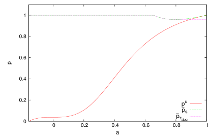
Figure 10: upper bound of transformation probability from $\ket{\phi}$ to $\ket{\psi}$

Lemma 4.

For a transformation from a tripartite state $\ket{\phi_{i}}$ to another tripartite state $\ket{\phi_{s}}$, if the interference term of $\ket{\phi_{i}}$ is not equal with $\ket{\phi_{s}}$, we can get an upper bound for the supremum of the successful probability which is less than 1.

Proof: If the interference term is not equal, put into the Equation 65 , we know the maximal successful probability $p_{as}(x)$ can not reach one. Otherwise the conservation of interference term will be violated. In fact, as the magnitude of the interference term of branches where we stop become larger and larger, $p_{as}(x)$ gets closer and closer to one. However, at the same time the maximal 3-tangle of these branches will go to zero. As the destination state is in GHZ class, its 3-tangle is not zero. So we can always find one $|x|$, when the magnitude square of the interference term reaches it, $max(\tau_{ABC}(\phi||I(\phi)|=|x|))<\tau_{ABC}(\phi_{s})$, then it will give an upper bound for this transformation which is smaller than 1. $\Box$

Remark 8.

One may naturally ask a question: If the interference terms of two states are the same, can we give an upper bound for the transformation probability? In this case, the above lemma can not give a nontrivial upper bound. However, we can still use other entanglement monotones, such as 3-tangle, to give an upper bound for the transformation from one to another.

Example 2.

Consider the transformation from $\ket{\phi}=\gamma(\ket{000}+\ket{abc})$ where $\braket{0}{a}=0.2$, $\braket{0}{b}=0.4$, $\braket{0}{c}=0.8$, to $\ket{\psi}=\gamma^{\prime}(\ket{000}+\ket{a^{\prime}b^{\prime}c^{\prime}})$ where $\braket{0}{a^{\prime}}=0.4$, $\braket{0}{b^{\prime}}=0.4$, $\braket{0}{c^{\prime}}=0.4$. One can check that $I(\ket{\phi})=I(\ket{\psi})=0.0602$. So naively we can only get a trivial upper bound for the transformation between them. However, notice that $\tau_{ABC}(\ket{\phi})=0.2564$ and $\tau_{ABC}(\psi)=0.5235$, we can get an upper bound for the transformation from $\ket{\phi}$ to $\ket{\psi}$ which is

$$\frac{\tau_{ABC}(\ket{\phi})}{\tau_{ABC}(\ket{\psi})}=\frac{0.2546}{0.5235}=0.4863<1$$ (70)

V Lower Bound for the Transformation

After the discussion about the upper bound, we have a question: Is this upper bound tight or not? Or can we find a transformation protocol that can reach such a transformation probability? In Chitambar2008 , they have provided a straight forward protocol: That is, if we want to transform

$$\ket{\mathrm{GHZ}}=\frac{1}{\sqrt{2}}(\ket{000}+\ket{111})$$

$$\stackrel{{\scriptstyle\textrm{LOCC}}}{{\longrightarrow}}\ket{\Psi} =\sqrt{K}(\ket{000}+\ket{\varphi_{A}}\ket{\varphi_{B}}\ket{\varphi_{C}}),$$ (71)

We can let Alice perform the measurement $\{\frac{A}{\|A\|},\sqrt{\mathbbm{1}-\frac{1}{\|A\|^{2}}A^{+}A}\}$, where

$$A\ket{0}=\ket{0},A\ket{1}=\ket{\varphi_{A}}$$ (72)

and similarly for Bob and Charlie. Then the final successful probability is $\frac{(1+c_{\alpha}c_{\beta}c_{\gamma})^{3}}{(1+c_{\alpha})(1+c_{\beta})(1+c_{\gamma})}$.

In the following, we will provide a transformation protocol that can transform GHZ-state generalized to n parties and m dimensions to other states with the same dimension and Schmidt rank with a probability higher than the straight forward protocol . However, there is still a gap between the upper bound and the lower bound we get. A surprising result derived from that is all tripartite pure 3-qubit states can be transformed from GHZ-state generalized to 3 parties and 3 dimensions by LOCC with probability 1, which was not known before.

We have found a lower bound for the maximum value of the transformation probability from GHZ state to $\ket{\Psi}$= $\gamma(\alpha\ket{a_{1}b_{1}c_{1}}+\beta\ket{a_{2}b_{2}c_{2}})$ by an explicit method, which we call four-step method.

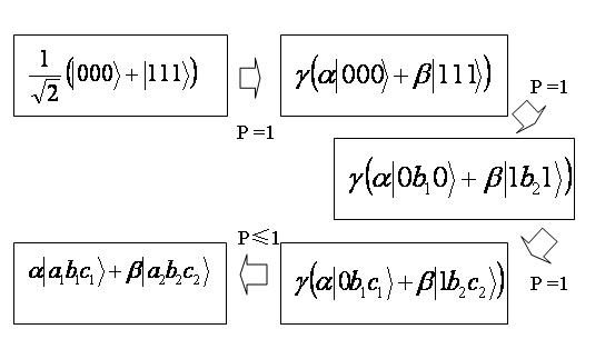
Figure 11: Four-step method

See Figure 11 for the process, in the first step, we transform GHZ state into $\ket{GHZ^{\prime}}=\alpha\ket{000}+\beta\ket{111}$ which has the same coefficient of terms (but different states) as $\ket{\Psi}$. Secondly, we transform $\ket{GHZ^{\prime}}$ into $\ket{\phi_{b1}}=\alpha\ket{0b_{1}0}+\beta\ket{1b_{2}1}$. Then we transform $\ket{\phi_{b1}}$ into $\ket{\phi_{c1}}=\alpha\ket{0b_{1}c_{1}}+\beta\ket{1b_{2}c_{2}}$. We will show the first three steps can be done with probability 1. Then if $\braket{a_{1}}{a_{2}}$ is zero, $\ket{\phi_{c1}}$ is unitary equivalent with $\ket{\Psi}$ so we can get $\ket{\Psi}$ with probability 1. In other cases, we can still get $\ket{\Psi}$ with a higher probability than the previous result in Chitambar2008 by performing an appropriate measurement.

In fact, the first step is a generalization of Nielsen Majorization result Nielsen1999 and Lo-Popescu’s Lo2001 result for the maximum probability of distilling a maximally entangled state. It has been noted previously in Xin2007 .

Definition 3.

A GHZ-like (aka Schmidt decomposable) state is a tripartite state that can be written in the form

$$\ket{\Psi}=\sum_{i}\lambda_{i}\ket{i}\ket{i}\ket{i}$$ (73)

Theorem 1 of Lo-Popescu also holds for the GHZ-like state, because it gives a bound for the case where the Bob-Charlie alliance is allowed to perform any (non-local) operations, and when the allowed operations are restricted to the subclass of local operations, the upper bound still has to hold.

Theorem 2(a) of Lo-Popescu can in the same way be applied to GHZ-like (Schmidt decomposable) states, because all unitary transformations on Bob’s side involve only a relabeling of the basis states ($\ket{i}\leftrightarrow\ket{j}$), and therefore extending it to GHZ-like states just changes this step to ($\ket{i}\ket{i}\leftrightarrow\ket{j}\ket{j}$), which can also be done by local unitaries only.

Theorem 2(b) generalizes to GHZ-like states as well, because here Alice performs all the operations and Bob either has to perform no operation on his state at all (result ”success”), or he has to discard it completely (result ”failure”), which can also be done if Bob’s state is distributed among Bob and Charlie.

In Xin2007 , it was shown that Nielsen’s majorization idea generalized to more parties can be applied to GHZ-like state, which means the transformation

$$\begin{split}\ket{GHZmn}=\frac{1}{\sqrt{m}}\sum^{m}_{i=1}\ket{i}_{1}\ket{i}_{2}...\ket{i}_{n}\\ \rightarrow\ket{\Psi}=\sum^{m}_{i=1}\alpha_{i}\ket{i}_{1}\ket{i}_{2}...\ket{i}_{n}\end{split}$$ (74)

can success with probability 1.

For the second and third step, we have the following lemma.

Lemma 5.

Turgut2009 The GHZ state can be transformed to $\ket{\Psi}$= $\gamma(\alpha\ket{a_{1}b_{1}c_{1}}+\beta\ket{a_{2}b_{2}c_{2}})$, where $\braket{\Psi}{\Psi}=1$ with probability 1, if $\ket{a_{1}b_{1}c_{1}}$ and $\ket{a_{2}b_{2}c_{2}}$ are orthogonal to each other.

Proof: Suppose $\ket{a_{1}}$ and $\ket{a_{2}}$ are orthogonal to each other. If we choose the basis in which $\ket{a_{1}b_{1}c_{1}}=\ket{000}$ then we write $\ket{\phi}=\gamma(\alpha\ket{000}+\beta\ket{1}_{A}(d_{1}\ket{0}+d_{2}\ket{1})_{B}(e_{1}\ket{0}+e_{2}\ket{1})_{C})$, where $|d_{1}|^{2}+|d_{2}|^{2}=1$ and $|e_{1}|^{2}+|e_{2}|^{2}=1$, in this case we can see $\gamma=1$

Then we can do the transformation in the following way.

Firstly, use the result of the first step to transform $\ket{GHZ}$ into $\ket{GHZ^{\prime}}=\alpha\ket{000}+\beta\ket{111}$ with probability 1.

Secondly, Bob performs a POVM

$$M_{1}=\frac{1}{\sqrt{2}}\left(\begin{array}[]{cc}1&d_{1}\\ 0&d_{2}\end{array}\right),\qquad M_{2}=\frac{1}{\sqrt{2}}\left(\begin{array}[]{cc}1&-d_{1}\\ 0&-d_{2}\end{array}\right),$$ (75)

Then with probability $\frac{1}{2}$ we get $\ket{\phi_{b1}}=\alpha\ket{000}+\beta\ket{1}_{A}(d_{1}\ket{0}+d_{2}\ket{1})_{B}\ket{1}_{C}$, and with probability $\frac{1}{2}$ we get $\ket{\phi_{b2}}=\alpha\ket{000}-\beta\ket{1}_{A}(d_{1}\ket{0}+d_{2}\ket{1})_{B}\ket{1}_{C}$. If we get $\ket{\phi_{b2}}$, Alice perform a unitary transformation

$$U_{A}=\left(\begin{array}[]{cc}1&0\\ 0&-1\end{array}\right),\qquad$$ (76)

then we get $\ket{\phi_{b1}}$, too. So, with probability 1 we get $\ket{\phi_{b1}}$.

Thirdly, Charlie performs a POVM

$$M_{1}=\frac{1}{\sqrt{2}}\left(\begin{array}[]{cc}1&e_{1}\\ 0&e_{2}\end{array}\right),\qquad M_{2}=\frac{1}{\sqrt{2}}\left(\begin{array}[]{cc}1&-e_{1}\\ 0&-e_{2}\end{array}\right),$$ (77)

Then with probability $\frac{1}{2}$ we get $\ket{\phi_{c_{1}}}=\alpha\ket{000}+\beta\ket{1}_{A}(d_{1}\ket{0}+d_{2}\ket{1})_{B}(e_{1}\ket{0}+e_{2}\ket{1})_{C}$, which is exactly the $\ket{\phi}$ we want to get, and with probability $\frac{1}{2}$ we can get $\ket{\phi_{c_{2}}}=\alpha\ket{000}-\beta\ket{1}_{A}(d_{1}\ket{0}+d_{2}\ket{1})_{B}(e_{1}\ket{0}+e_{2}\ket{1})_{C}$. If we get $\ket{\phi_{c_{2}}}$, again, Alice can perform a unitary transformation

$$U_{A}=\left(\begin{array}[]{cc}1&0\\ 0&-1\end{array}\right),\qquad$$ (78)

to get $\ket{\phi_{c1}}$, too. So with probability 1 we can get $\ket{\phi_{c1}}$. Then we can get $\ket{\Psi}$= $\alpha\ket{a_{1}b_{1}c_{1}}+\beta\ket{a_{2}b_{2}c_{2}}$ with certainty. $\Box$

Then we show the first three steps can be done with probability 1. For the last step, we have the following lemma.

Lemma 6.

For $\ket{\Psi}$= $\gamma(\alpha\ket{a_{1}b_{1}c_{1}}+\beta\ket{a_{2}b_{2}c_{2}})$, where $\alpha^{2}+\beta^{2}=1$ and $\gamma$ is a normalization factor, if $<a_{1}|a_{2}>$=$\lambda_{a}$, $<b_{1}|b_{2}>$=$\lambda_{b}$,$<c_{1}|c_{2}>$=$\lambda_{c}$, then there exists an LOCC transformation protocol from GHZ state to $\ket{\psi}$ such that the probability of success is at least $\frac{1+2\alpha\beta\lambda_{a}\lambda_{b}\lambda_{c}}{1+\lambda_{m}}$, where $\lambda_{m}$= $min(\lambda_{a},\lambda_{b},\lambda_{c})$.

Proof: Firstly, we have $\ket{\psi}=\gamma(\alpha\ket{000}+\beta(\lambda_{a}\ket{0}+\sqrt{1-\lambda^{2}_{a}}\ket{1})_{A}(\lambda_{b}\ket{0}+\sqrt{1-\lambda^{2}_{b}}\ket{1})_{B}(\lambda_{c}\ket{0}+\sqrt{1-\lambda^{2}_{c}}\ket{1})_{C})$, where $\gamma=\frac{1}{\sqrt{1+2\alpha\beta\lambda_{a}\lambda_{b}\lambda_{c}}}$. From theorem 1, we transform GHZ state to $\ket{\xi}=\alpha\ket{000}+$ $\beta\ket{1}_{A}(\lambda_{b}\ket{0}$ $+\sqrt{1-\lambda^{2}_{b}}\ket{1})_{B}$ $(\lambda_{c}\ket{0}+\sqrt{1-\lambda^{2}_{c}}\ket{1})_{C}$, with probability 1. Then from $\ket{\xi}$, Alice can do a POVM

$$M_{1}=\frac{1}{\sqrt{1+\lambda_{a}}}\left(\begin{array}[]{cc}1&\lambda_{a}\\ 0&\sqrt{1-\lambda^{2}_{a}}\end{array}\right),\qquad$$ (81)

$$M_{2}=\frac{\sqrt{\lambda_{a}}}{\sqrt{1+\lambda_{a}}}\left(\begin{array}[]{cc}1&-1\\ 0&0\end{array}\right),$$ (84)

So we have probability $\frac{1+2\alpha\beta\lambda_{a}\lambda_{b}\lambda_{c}}{1+\lambda_{a}}$ to get $\ket{\psi}$, and the other branch will give a state in which the rank of $\rho_{a}$ is 1 so that the probability to get $\ket{\psi}$ from it is zero. Then the total probability is $\frac{1+2\alpha\beta\lambda_{a}\lambda_{b}\lambda_{c}}{1+\lambda_{a}}$. However, we can do a permutation of A, B and C so that the probability can also be $\frac{1+2\alpha\beta\lambda_{a}\lambda_{b}\lambda_{c}}{1+\lambda_{b}}$ and $\frac{1+2\alpha\beta\lambda_{a}\lambda_{b}\lambda_{c}}{1+\lambda_{c}}$. And the maximum probability corresponds to $min(\lambda_{a},\lambda_{b},\lambda_{c})$. $\Box$

Example 3.

Again take the transformation from $\ket{GHZ}$ to $\ket{\phi}=\gamma(\ket{000}+\ket{aaa})$, where $\ket{a}=c\ket{0}+\sqrt{1-c^{2}}\ket{1}$ and $c\in(0,1]$ as an example, using the protocol we provide, we can get a successful probability $\frac{1+c^{3}}{1+c}$, let c=0.5, we have $p_{s}=0.7500$. In comparison, the upper bound we get in section 3 is 0.9604. There is still a gap between these two values. How to reduce it is still an open problem.

Now we will generalize the result of lemma 5 higher dimensions and more parties. Suppose we are concerned with the transformation from the GHZ-state generalized to n parties and m dimensions, $\ket{GHZmn}=\frac{1}{\sqrt{m}}\sum^{m}_{i=1}\ket{i}_{1}\ket{i}_{2}...\ket{i}_{n}$ to $\ket{\psi}$= $\gamma(\sum^{m}_{i=1}\alpha_{i}\ket{k_{1_{i}}k_{2_{i}}...k_{n_{i}}})$. The basic idea of our protocol can be divided into three steps: Firstly, we would like to transform $\ket{GHZmn}$ into $\ket{\Psi}=\sum^{m}_{i=1}\alpha_{i}\ket{i}\ket{i}\ket{i}$ which is called GHZ-like (or Schmidt decomposable) state. Secondly, we transform $\ket{\Psi}$ into $\ket{\psi_{n}}$ = $\sum^{m}_{i=1}\alpha_{i}\ket{i_{1}k_{2_{i}}k_{i_{3}}...k_{i_{n}}}$. We will show these two steps can be done with probability 1. Finally, if for at least m-1 terms of $\ket{\psi}$, there can be at least one party with a state that is orthogonal to this party’s state in every other term, our protocol can transform $\ket{GHZmn}$ into $\ket{\psi}$ with probability 1. In other cases, our protocol can be done with a probability higher than what have been known before.

The second and third step for the case when for at least m-1 terms of $\ket{\psi}$, there can be at least one party with a state that is orthogonal to this party’s state in every other term are incorporated in the following theorem.

Theorem 10.

The GHZ-state generalized to n parties and m dimensions, $\ket{GHZmn}=\frac{1}{\sqrt{m}}\sum^{m}_{i=1}\ket{i}_{1}\ket{i}_{2}...\ket{i}_{n}$, can be transformed to $\ket{\psi}$= $\sum^{m}_{i=1}\alpha_{i}\ket{k_{1_{i}}k_{2_{i}}...k_{n_{i}}}$ with probability 1, if $\exists$ p, $\forall$ i$\neq$ p, $\exists$ j with $\braket{k_{j_{i}}}{k_{j_{l}}}=0$ for $\forall$ $l\neq i$. This means for at least m-1 terms, there has to be at least one party with a state that is orthogonal to this party’s state in every other term.

Proof: The basic idea is we at first make the coefficient of each term equal to the corresponding terms of the destination state. Then let party 2 perform a POVM which transforms the state into many states in such a form: for each term, the party 2 part of the term is the same with the destination state, but the term’s coefficient maybe of the same or the opposite sign of the destination state. Then by introducing a unitary transformation on the party 1, we can make all the coefficients the same with the destination state. Keep doing this for party 3, $\cdot$, n. Finally, do a similar POVM on party 1, we can get many states in such a form: the corresponding terms are the same, but the coefficients may be of the same or the opposite sign. Then we can use unitary transformation to transform all the states into the destination state. Exact process is in the following:

Firstly, using the result of Xin2007 to get $\ket{GHZmn}=\gamma(\sum^{m}_{i=1}\alpha_{i}\ket{i}_{1}\ket{i}_{2}...\ket{i}_{n})$ where $\gamma$ is a normalization factor. But then, the POVMs should be modified. We call the parties 1,2, $\cdots$, n party 1, party 2, and so on. Take Party 2 as an example, suppose with a unitary transformation, $\ket{k_{2_{i}}}=\sum^{i}_{j=0}a_{2_{ij}}\ket{j}_{2}$, in which $a_{2_{00}}=1$, then party 2 can operate a POVM

$$\begin{split}&M_{0}=\frac{1}{\sqrt{2^{m-1}}}\left(\begin{array}[]{ccccc}1&a_{2_{10}}&\cdots&a_{2_{(m-1)0}}\\ 0&a_{2_{11}}&\cdots&a_{2_{(m-1)1}}\\ \vdots&\vdots&\vdots&\vdots\\ 0&0&\cdots&a_{2_{(m-1)(m-1)}}\end{array}\right),\qquad\\ &M_{1}=\frac{1}{\sqrt{2^{m-1}}}\left(\begin{array}[]{ccccc}1&a_{2_{10}}&\cdots&-a_{2_{(m-1)0}}\\ 0&a_{2_{11}}&\cdots&-a_{2_{(m-1)1}}\\ \vdots&\vdots&\vdots&\vdots\\ 0&0&\cdots&-a_{2_{(m-1)(m-1)}}\end{array}\right),\qquad\\ &\vdots\\ &M_{2^{m-1}-1}=\frac{1}{\sqrt{2^{m-1}}}\left(\begin{array}[]{ccccc}1&-a_{2_{10}}&\cdots&-a_{2_{(m-1)0}}\\ 0&-a_{2_{11}}&\cdots&-a_{2_{(m-1)1}}\\ \vdots&\vdots&\vdots&\vdots\\ 0&0&\cdots&-a_{2_{(m-1)(m-1)}}\end{array}\right)\end{split}$$ (85)

Then we can get a state unitary equivalent with $\ket{\psi_{2}}$= $\sum^{m}_{i=1}\alpha_{i}\ket{i_{1}k_{i_{2}}i_{3}...i_{n}}$ with probability $\frac{1}{2^{m-1}}$ and with the same probability we get other states which are different with $\ket{\psi_{2}}$ just because some terms have an opposite sign than the corresponding terms in $\ket{\psi_{2}}$.

And we do a unitary transformation on party 1 to transform all branches into $\ket{\psi_{2}}$. For party 3,4, $\cdots$ n, we can use similar method, so at last we can get a state unitary equivalent with $\ket{\psi_{n}}$= $\sum^{m}_{i=1}\alpha_{i}\ket{i_{1}k_{2_{i}}k_{i_{3}}...k_{i_{n}}}$. Then we finish the second step with probability 1.

After that, party 1 can perform a similar POVM and with probability $\frac{1}{2^{m-1}}$ we get $\ket{\psi}$ which we want and with the same probability we get other states which are different with $\ket{\psi}$ just because some terms have an opposite sign than the corresponding terms in $\ket{\psi}$.

However, if for at least m-1 terms, there is at least one party with a state, which we call $\ket{k_{i_{j}}}$, that is orthogonal to this party’s state in every other term, we can introduce a minus sign for this term by a unitary transformation of party j which transforms $\ket{k_{i_{j}}}$ to $-\ket{k_{i_{j}}}$ and do nothing to all the other states orthogonal to $\ket{k_{i_{j}}}$. Thus we can introduce a minus sign for these m-1 terms just by unitary transformation. For the only one term which does not have this property (if it exists), we can introduce a minus sign for every other term and then multiply -1 for the whole wave function. Then, we can get $\ket{\psi}$ with probability 1. $\Box$

Remark 9.

The condition we require in Lemma 10 is different from each term is orthogonal to other ones. In fact, it is a stronger requirement than orthogonality. See the example below: for a state $\ket{\phi}=\frac{1}{\sqrt{3}}[\ket{000}+\ket{1}(\ket{0}+\ket{1})\ket{0}+(\ket{0}+\ket{1})\ket{0}\ket{1}]$, it is easy to check each term is orthogonal to another in this state. But we do not know how to introduce a minus sign for any term because the condition in Lemma 1 is not satisfied.

There is an open question: Can this condition in Lemma 2 be ”if and only if” in higher dimensions? To make it also ”only if”, there are two problems: 1. Is the form we write the state still unique in higher dimensions? We know, for a 2-term tripartite state in which each party has rank 2, if we write it in the form $\ket{\psi}=\gamma(\alpha\ket{000}+\beta(\lambda_{a}\ket{0}+\sqrt{1-\lambda^{2}_{a}}\ket{1})_{A}(\lambda_{b}\ket{0}+\sqrt{1-\lambda^{2}_{b}}\ket{1})_{B}(\lambda_{c}\ket{0}+\sqrt{1-\lambda^{2}_{c}}\ket{1})_{C})$, the result should be unique. It is also true for a 3-term tripartite state (the W-class state) Ac'in2000 , but the similar result for the higher dimension conditions have not been proved. 2. Can a state in which all terms are orthogonal to each other be transformed from GHZ like state with probability 1? We know, our protocol can only work for a stronger requirement. However, for states with orthogonal terms, the inner product is also zero, so how can we prove the probability can not be one in this case is another problem.

Corollary 3.

All tripartite pure three qubit states can be transformed from 3-term GHZ state $\frac{1}{\sqrt{3}}(\ket{000}+\ket{111}+\ket{222})$ with probability 1.

Proof: From the paper Ac'in2000 , we know any tripartite pure state can be written as

$$\begin{split}\ket{\Phi}=&\lambda_{0}\ket{000}+\lambda_{1}e^{i\phi}\ket{100}+\lambda_{2}|101>\\ &+\lambda_{3}\ket{110}+\lambda_{4}\ket{111},\\ &\lambda_{i}\geq 0,0\leq\phi\leq\pi,\mu_{i}\equiv\lambda^{2}_{i},\sum{\mu_{i}}=1\end{split}$$ (86)

And shown in Ac'in2000 , if Charlie introduces a unitary transformation

$$U=\frac{1}{\sqrt{\mu_{1}+\mu_{2}}}\left(\begin{array}[]{cc}\lambda_{1}e^{-i\phi}&\lambda_{2}e^{-i\phi}\\ \lambda_{2}&-\lambda_{1}\end{array}\right),$$ (87)

we can get

$$\begin{split}\ket{\Psi}=&\frac{1}{\sqrt{\mu_{1}+\mu_{2}}}[e^{-i\phi}\lambda_{0}\lambda_{1}\ket{000}+e^{-i\phi}\lambda_{0}\lambda_{2}\ket{001}\\ &+(\lambda_{1}^{2}+\lambda_{2}^{2})\ket{100}+(\lambda_{1}\lambda_{3}+\lambda_{2}\lambda_{4})\ket{110}\\ &+(\lambda_{2}\lambda_{3}-\lambda_{1}\lambda_{4})\ket{111}]\end{split}$$ (88)

which is unitary equivalent with the state we want.

If we combine the first and second term into a term and do the same for third and fifth term we can get $|\Psi>=\ket{00}(a\ket{0}+b\ket{1})+d\ket{100}+\ket{11}(c\ket{0}+e\ket{1})$, easy to see, if we consider it as a 3-term state, it satisfies the condition we required for Lemma 2, (Alice in first term and Bob in third term), so we can transform it from 3-term GHZ generalized state with probability 1. $\Box$

Theorem 11.

For a general $\ket{\psi}$= $\gamma(\sum^{m}_{i=1}\alpha_{i}\ket{k_{1_{i}}k_{2_{i}}...k_{n_{i}}}),$ where $\sum^{m}_{i=1}\alpha^{2}_{i}=1$ and $\gamma$ is the normalization factor. There exists an LOCC transformation protocol from the GHZ-state generalized to n parties and m dimensions, $\ket{GHZmn}=\frac{1}{\sqrt{m}}\sum^{m}_{i=1}\ket{i}_{1}\ket{i}_{2}...\ket{i}_{n}$ to $\ket{\psi}$ such that the probability of success is at least $max(\frac{1}{\gamma||A_{i}||^{2}})$, where

$$A_{i}=\frac{1}{\sqrt{2^{m-1}}}\left(\begin{array}[]{ccccc}1&a_{i_{10}}&\cdots&a_{i_{(m-2)0}}&a_{i_{(m-1)0}}\\ 0&a_{i_{11}}&\cdots&a_{i_{(m-2)1}}&a_{i_{(m-1)1}}\\ \vdots&\vdots&\vdots&\vdots&\vdots\\ 0&0&\cdots&0&a_{i_{(m-1)(m-1)}}\end{array}\right)$$ (89)

Proof: To generalize theorem 2 to general m-term n-party states, we can firstly get $\ket{\psi_{n}}$= $\sum^{m}_{i=1}\alpha_{i}\ket{i_{1}k_{i_{2}}k_{i_{3}}...k_{i_{n}}}$ with certainty. And Alice perform a POVM $\{\frac{A_{1}}{||A_{1}||},\sqrt{1-\frac{A_{1}^{+}A_{1}}{||A_{1}||^{2}}}\}$, where

$$A_{1}=\frac{1}{\sqrt{2^{m-1}}}\left(\begin{array}[]{ccccc}1&a_{1_{10}}&\cdots&a_{1_{(m-2)0}}&a_{1_{(m-1)0}}\\ 0&a_{1_{11}}&\cdots&a_{1_{(m-2)1}}&a_{1_{(m-1)1}}\\ \vdots&\vdots&\vdots&\vdots&\vdots\\ 0&0&\cdots&0&a_{1_{(m-1)(m-1)}}\end{array}\right)$$ (90)

After calculation we can find the successful probability is $\frac{1}{\gamma||A_{1}||^{2}}$. Similarly, we can choose other party to finish the final step and find the best one which give the maximum transformation probability.

VI Summary and Concluding Remarks

We derive upper bound and lower bound for the supremum transformation probability from GHZ state to GHZ-class state. In the derivation of the upper bounds, we consider the action of the LOCC protocol on a different input state, namely $1/\sqrt{2}[\ket{000}-\ket{111}]$, and demand that the probability of an outcome remains bounded by 1. By considering the constraints of the interference term and 3-tangle, we find an upper bound for more general cases. For the lower bound, we construct a new transformation protocol: the four-step method to do the transformation. Before that, there was no nontrivial upper bound known for this transformation. Based on the previous results of weak measurement, we construct a ”stop and reconstruct” method which may be very useful in the analyzation of the LOCC transformation protocols. The lower bound is generalized into higher dimension. During the discussion of lower bound, we find all tripartite pure 3-qubit states can be transformed from $\ket{GHZ_{23}}=\frac{1}{\sqrt{3}}(\ket{000}+\ket{111}+\ket{222})$ with probability 1. This is a new result.

There are still open questions and possible future generalization of the result we have, which is mentioned during the above discussion. To summarize, firstly, there is still a gap between the upper bound and lower bound we get. How to further decrease the gap and finally find the optimum transformation protocol are still open questions. Secondly, we want to generalize the upper bound we get to higher dimension. To do this, we need firstly make sure the GHZ-class state generalized into the higher dimension is still unique so that we can still talk about the inner product. We also need to find the corresponding entanglement monotone for higher dimension case. Finally, the result of Corollary 1 is very surprising, one question is whether it can be generalized into higher dimension case. To do this, we need to analyze the Generalized Schmidt Decomposition in higher dimension Tamaryan2008 or other forms to express the state in higher dimensions Verstraete2002 .

VII Appendix: Proof of Theorem 5

Proof: From the formula of the two quantity:

$$I= \frac{2c_{\alpha}c_{\beta}c_{\gamma}s_{\delta}c_{\delta}c_{\varphi}}{1+2c_{\alpha}c_{\beta}c_{\gamma}s_{\delta}c_{\delta}c_{\varphi}}$$ (91)

$$I^{2}= \frac{4c^{2}_{\alpha}c^{2}_{\beta}c^{2}_{\gamma}s^{2}_{\delta}c^{2}_{\delta}c^{2}_{\varphi}}{(1+2c_{\alpha}c_{\beta}c_{\gamma}s_{\delta}c_{\delta}c_{\varphi})^{2}}$$ (92)

$$\tau_{ABC}= \frac{4s^{2}_{\alpha}s^{2}_{\beta}s^{2}_{\gamma}s^{2}_{\delta}c^{2}_{\delta}}{(1+2c_{\alpha}c_{\beta}c_{\gamma}s_{\delta}c_{\delta}c_{\varphi})^{2}}$$ (93)

We have

$$\tau_{ABC}= I^{2}\frac{s^{2}_{\alpha}s^{2}_{\beta}s^{2}_{\gamma}}{c^{2}_{\alpha}c^{2}_{\beta}c^{2}_{\gamma}c^{2}_{\varphi}}$$

$$= I^{2}\frac{(1-c^{2}_{\alpha})(1-c^{2}_{\beta})(1-c^{2}_{\gamma})}{c^{2}_{\alpha}c^{2}_{\beta}c^{2}_{\gamma}c^{2}_{\varphi}}$$ (95)

We consider the condition when $I>0$ at first.

Firstly, we consider the condition when $s_{\delta}=c_{\delta}=\frac{\sqrt{2}}{2},c_{\varphi}=1$. In this case, we have $c_{\alpha}c_{\beta}c_{\gamma}=\frac{I}{1-I}$. let $\frac{I}{1-I}=a^{3}$ where $a=(\frac{I}{1-I})^{\frac{1}{3}}$. Then we have

$$\tau_{ABC}= I^{2}\frac{(1-c^{2}_{\alpha})(1-c^{2}_{\beta})(1-c^{2}_{\gamma})}{c^{2}_{\alpha}c^{2}_{\beta}c^{2}_{\gamma}}$$

$$= I^{2}\frac{(1-c^{2}_{\alpha})(1-c^{2}_{\beta})(1-\frac{a^{6}}{c^{2}_{\alpha}c^{2}_{\beta}})}{a^{6}}$$ (96)

Take partial derivation of $c_{\alpha}$ and $c_{\beta}$ we can find this expression reaches its maximum value when $c_{\alpha}=c_{\beta}=c_{\gamma}=a$ and the corresponding maximum value of 3-tangle is $\tau_{{ABC}_{0}}=((1-I)^{\frac{2}{3}}-I^{\frac{2}{3}})^{3}=\frac{(1-a^{2})^{3}}{(1+a^{3})^{2}}$.

Now we will show in other cases when $s_{\delta}\neq c_{\delta}orc_{\varphi}<1$, we can only get a 3-tangle smaller than $\tau_{{ABC}_{0}}$.

If $s_{\delta}\neq c_{\delta}$, we will have $s_{\delta}c_{\delta}<\frac{1}{2}$, then from the expression of I we can find $c_{\alpha}c_{\beta}c_{\gamma}c_{\varphi}>\frac{I}{1-I}=a^{3}$, then as $c_{\varphi}\leq 1$, we also have $c_{\alpha}c_{\beta}c_{\gamma}=b^{3}>a^{3}$. And also take the partial derivation of $(1-c^{2}_{\alpha})(1-c^{2}_{\beta})(1-c^{2}_{\gamma})$ we can find its maximum value is $(1-b^{2})^{3}<(1-a^{2})^{3}$. Finally we have

$$\tau_{ABC}= I^{2}\frac{(1-c^{2}_{\alpha})(1-c^{2}_{\beta})(1-c^{2}_{\gamma})}{c^{2}_{\alpha}c^{2}_{\beta}c^{2}_{\gamma}c^{2}_{\varphi}}$$

$$< I^{2}\frac{(1-a^{2})^{3}}{a^{6}}=\frac{(1-a^{2})^{3}}{(1+a^{3})^{2}}=\tau_{{ABC}_{0}}$$ (97)

That is to say, when $s_{\delta}\neq c_{\delta}$, $\tau_{ABC}$ is always smaller than $\tau_{{ABC}_{0}}$. Now let us consider the case when $s_{\delta}=c_{\delta}=\frac{\sqrt{2}}{2}$, but $c_{\varphi}<1$.

Then again we have $c_{\alpha}c_{\beta}c_{\gamma}c_{\varphi}=\frac{I}{1-I}=a^{3}$. But as $c_{\varphi}<1$, we still have $c_{\alpha}c_{\beta}c_{\gamma}=d^{3}>a^{3}$. And also take the partial derivation of $(1-c^{2}_{\alpha})(1-c^{2}_{\beta})(1-c^{2}_{\gamma})$ we can find its maximum value is $(1-d^{2})^{3}<(1-a^{2})^{3}$. So we have

$$\tau_{ABC}= I^{2}\frac{(1-c^{2}_{\alpha})(1-c^{2}_{\beta})(1-c^{2}_{\gamma})}{c^{2}_{\alpha}c^{2}_{\beta}c^{2}_{\gamma}c^{2}_{\varphi}}=I^{2}\frac{(1-d^{2})^{3}}{a^{6}}$$

$$< I^{2}\frac{(1-a^{2})^{3}}{a^{6}}=\frac{(1-a^{2})^{3}}{(1+a^{3})^{2}}=\tau_{{ABC}_{0}}$$ (98)

Then we show, for the interference term $I>0$, we have

$$max(\tau_{ABC}(\phi|I(\phi)=I>0))=\frac{(1-a^{2})^{3}}{(1+a^{3})^{2}}$$ (99)

When $I\leq 0$, the discussion is almost the same. Except that, we need to consider the condition $s_{\delta}=c_{\delta}=\frac{\sqrt{2}}{2},c_{\varphi}=-1$ first and find $c_{\alpha}c_{\beta}c_{\gamma}=-\frac{I}{1-I}=a^{\prime 3}>0$. Then easy to find the corresponding maximum value is $\frac{(1-a^{\prime 2})^{3}}{(1-a^{\prime 3})^{2}}$. And use the same tricks one can show it is the maximum value of the 3-tangle.

One thing to notice is that, the expression of a’ and a is just opposite to each other. So if we let $a=\frac{I}{1-I}=-a^{\prime}$ when $I\leq 0$, we will get

$$max(\tau_{ABC}(\phi|I(\phi)=I\leq 0))=\frac{(1-a^{\prime 2})^{3}}{(1-a^{\prime 3})^{2}}=\frac{(1-a^{2})^{3}}{(1+a^{3})^{2}}$$ (100)

Then in all we have

$$max(\tau_{ABC}(\phi|I(\phi)=I)=\frac{(1-a^{\prime 2})^{3}}{(1-a^{\prime 3})^{2}}=\frac{(1-a^{2})^{3}}{(1+a^{3})^{2}}$$ (101)

$\Box$.

References

- (1) C. H. Bennett, H. J. Bernsein, S. Popescu, and B. Schumacher, Phys. Rev. A 53, 2046 (1996).
- (2) H.-K. Lo and S. Popescu, Phys. Rev. A 63, 022301 (2001).
- (3) M. A. Nielsen, Physical Review Letters 83, 436 (1999).
- (4) G. Vidal, Phys. Rev. Lett. 83, 1046 (1999).
- (5) W. Dür, G. Vidal, and J. I. Cirac, Phys. Rev. A 62, 062314 (2000).
- (6) F. Verstraete, J. Dehaene, B. De Moor, and H. Verschelde, Phys. Rev. A 65, 052112 (2002).
- (7) A. Acín, E. Jané, W. Dür, and G. Vidal, Phys. Rev. Lett. 85, 4811 (2000).
- (8) S. Turgut, Y. Gul, and N. K. Pak, arXiv:0907.3960v2 (2009).
- (9) J. Eisert and H. J. Briegel, Phys. Rev. A 64, 022306 (2001).
- (10) A. Acín et al., Phys. Rev. Lett. 85, 1560 (2000).
- (11) V. Coffman, J. Kundu, and W. K. Wootters, Phys. Rev. A 61, 052306 (2000).
- (12) O. Oreshkov and T. A. Brun, Physical Review Letters 95, 110409 (2005).
- (13) E. Andersson and D. K. L. Oi, arXiv:0712.2665 (2007).
- (14) E. Chitambar, R. Duan, and Y. Shi, Phys. Rev. Lett. 101, 140502 (2008).
- (15) Y. Xin and R. Duan, arxiv:0707.1947 (2007).
- (16) L. Tamaryan, D. Park, and S. Tamaryan, (2008).