b-Bit Minwise Hashing

Abstract

This paper establishes the theoretical framework of $b$-bit minwise hashing. The original minwise hashing method[3] has become a standard technique for estimating set similarity (e.g., resemblance) with applications in information retrieval, data management, social networks and computational advertising.

By only storing the lowest $b$ bits of each (minwise) hashed value (e.g., $b=1$ or 2), one can gain substantial advantages in terms of computational efficiency and storage space. We prove the basic theoretical results and provide an unbiased estimator of the resemblance for any $b$. We demonstrate that, even in the least favorable scenario, using $b=1$ may reduce the storage space at least by a factor of 21.3 (or 10.7) compared to using $b=64$ (or $b=32$), if one is interested in resemblance $\geq 0.5$.

1 Introduction

Computing the size of set intersections is a fundamental problem in information retrieval, databases, and machine learning. Given two sets, $S_{1}$ and $S_{2}$, where

$$S_{1},S_{2}\subseteq\Omega=\{0,1,2,...,D-1\},$$

a basic task is to compute the joint size $a=|S_{1}\cap S_{2}|$, which measures the (un-normalized) similarity between $S_{1}$ and $S_{2}$. The so-called resemblance, denoted by $R$, provides a normalized similarity measure:

$$R=\frac{|S_{1}\cap S_{2}|}{S_{1}\cup S_{2}|}=\frac{a}{f_{1}+f_{2}-a},\hskip 10.84006pt\text{where}\ f_{1}=|S_{1}|,\ f_{2}=|S_{2}|.$$

It is known that $1-R$, the resemblance distance, is a metric, i.e., satisfying the triangle inequality[3, 7].

In large datasets encountered in information retrieval and databases, efficiently computing the joint sizes is often highly challenging[2, 14]. Detecting (nearly) duplicate web pages is a classical example[3, 5].

Typically, each Web document can be processed as “a bag of shingles,” where a shingle consists of $w$ contiguous words in a document. Here $w$ is a tuning parameter and was set to be $w=5$ in several studies[3, 5, 10].

Clearly, the total number of possible shingles is huge. Considering merely $10^{5}$ unique English words, the total number of possible $5$-shingles should be $D=(10^{5})^{5}=O(10^{25})$. Prior studies used $D=2^{64}$ [10] and $D=2^{40}$[3, 5].

1.1 Minwise Hashing

In their seminal work, Broder and his colleagues developed minwise hashing and successfully applied the technique to the task of duplicate document removal at the Web scale[3, 5]. Since then, there have been considerable theoretical and methodological developments[15, 7, 16, 4, 19, 20, 21].

As a general technique for estimating set similarity, minwise hashing has been applied to a wide range of applications, for example, content matching for online advertising[24], detection of large-scale redundancy in enterprise file systems[11], syntactic similarity algorithms for enterprise information management[22], compressing social networks[8], advertising diversification[13], community extraction and classification in the Web graph[9], graph sampling[23], wireless sensor networks[18], Web spam[26, 17], Web graph compression [6], text reuse in the Web[1], and many more.

Here, we give a brief introduction to this algorithm. Suppose a random permutation $\pi$ is performed on $\Omega$, i.e.,

$$\pi:\ \Omega\longrightarrow\Omega,\hskip 21.68121pt\text{where}\ \ \ \Omega=\{0,1,...,D-1\}$$

An elementary probability argument can show

$$\mathbf{Pr}\left(\text{min}({\pi}(S_{1}))=\text{min}({\pi}(S_{2}))\right)=\frac{|S_{1}\cap S_{2}|}{|S_{1}\cup S_{2}|}=R.$$ (1)

After $k$ minwise independent permutations, denoted by $\pi_{1}$, $\pi_{2}$, …, $\pi_{k}$, one can estimate $R$ without bias, as a binomial probability, i.e.,

$$\hat{R}_{M}=\frac{1}{k}\sum_{j=1}^{k}1\{{\min}({\pi_{j}}(S_{1}))={\min}({\pi_{j}}(S_{2}))\},$$ (2)

$$\text{Var}\left(\hat{R}_{M}\right)=\frac{1}{k}R(1-R).$$ (3)

Throughout the paper, we will frequently use the term “sample,” corresponding to the term “sample size” (denoted by $k$). In minwise hashing, a sample is a hashed value, e.g., ${\min}({\pi_{j}}(S_{i}))$, which may require e.g., 64 bits to store[10], depending on the universal size $D$. The total storage for each set would be $bk$ bits, where $b=64$ is possible.

After the samples have been collected, the storage and computational cost is proportional to $b$. Therefore, reducing the number of bits for each hashed value would be useful, not only for saving significant storage space but also for considerably improving the computational efficiency.

1.2 Our Main Contributions

In this paper, we establish a unified theoretical framework for b-bit minwise hashing. Instead of using $b=64$ bits[10] or $40$ bits[3, 5], our theoretical results suggest using as few as $b=1$ or $b=2$ bits can yield significant improvements.

In $b$-bit minwise hashing, a “sample” consists of $b$ bits only, as opposed to e.g., 64 bits in the original minwise hashing.

Intuitively, using fewer bits per sample will increase the estimation variance, compared to (3), at the same “sample size” $k$. Thus, we will have to increase $k$ to maintain the same accuracy. Interestingly, our theoretical results will demonstrate that, when resemblance is not too small (e.g., $R\geq 0.5$, the threshold used in[3, 5]), we do not have to increase $k$ much. This means that, compared to the earlier approach, the b-bit minwise hashing can be used to improve estimation accuracy and significantly reduce storage requirements at the same time.

For example, when $b=1$ and $R=0.5$, the estimation variance will increase at most by a factor of 3 (even in the least favorable scenario). This means, in order not to lose accuracy, we have to increase the sample size by a factor of 3. If we originally stored each hashed value using 64 bits[10], the improvement by using $b=1$ will be $64/3=21.3$.

2 The Fundamental Results

Consider two sets, $S_{1}$ and $S_{2}$,

$$S_{1},S_{2}\subseteq\Omega=\{0,1,2,...,D-1\},$$

$$f_{1}=|S_{1}|,\ f_{2}=|S_{2}|,\ a=|S_{1}\cap S_{2}|$$

Apply a random permutation $\pi$ on $S_{1}$ and $S_{2}$: $\pi:\Omega\longrightarrow\Omega$. Define the minimum values under $\pi$ to be $z_{1}$ and $z_{2}$:

$$z_{1}=\min\left(\pi\left(S_{1}\right)\right),\hskip 14.45377ptz_{2}=\min\left(\pi\left(S_{2}\right)\right).$$

Define $e_{1,i}=i$th lowest bit of $z_{1}$, and $e_{2,i}=i$th lowest bit of $z_{2}$. Theorem 1 derives the analytical expression for $E_{b}$:

$$E_{b}=\mathbf{Pr}\left(\prod_{i=1}^{b}1\{e_{1,i}=e_{2,i}\}=1\right).$$ (4)

Theorem 1

Assume $D$ is large.

$$\mathbf{Pr}\left(\prod_{i=1}^{b}1\left\{e_{1,i}=e_{2,i}\right\}=1\right)=C_{1,b}+\left(1-C_{2,b}\right)R$$ (5)

where

$$r_{1}=\frac{f_{1}}{D},\hskip 14.45377ptr_{2}=\frac{f_{2}}{D},$$ (6)

$$C_{1,b}=A_{1,b}\frac{r_{2}}{r_{1}+r_{2}}+A_{2,b}\frac{r_{1}}{r_{1}+r_{2}},$$ (7)

$$C_{2,b}=A_{1,b}\frac{r_{1}}{r_{1}+r_{2}}+A_{2,b}\frac{r_{2}}{r_{1}+r_{2}},$$ (8)

$$A_{1,b}=\frac{r_{1}\left[1-r_{1}\right]^{2^{b}-1}}{1-\left[1-r_{1}\right]^{2^{b}}},$$ (9)

$$A_{2,b}=\frac{r_{2}\left[1-r_{2}\right]^{2^{b}-1}}{1-\left[1-r_{2}\right]^{2^{b}}}.$$ (10)

For a fixed $r_{j}$ (where $j\in\{1,2\}$), $A_{j,b}$ is a monotonically decreasing function of $b=1,2,3,...$.

For a fixed $b$, $A_{j,b}$ is a monotonically decreasing function of $r_{j}\in[0,1]$, with the limit to be

$$\lim_{r_{j}\rightarrow 0}A_{j,b}=\frac{1}{2^{b}}.$$ (11)

Proof: See Appendix A.$\Box$

Theorem 1 says that, for a given $b$, the desired probability (4) is determined by $R$ and the ratios, $r_{1}=\frac{f_{1}}{D}$ and $r_{2}=\frac{f_{2}}{D}$. The only assumption needed in the proof of Theorem 1 is that $D$ should be large, which is always satisfied in practice.

$A_{j,b}$ ($j\in\{1,2\}$) is a decreasing function of $r_{j}$ and $A_{j,b}\leq\frac{1}{2^{b}}$. As $b$ increases, $A_{j,b}$ converges to zero very quickly. In fact, when $b\geq 32$, one can essentially view $A_{j,b}=0$.

2.1 The Unbiased Estimator

Theorem 1 naturally suggests an unbiased estimator of $R$, denoted by $\hat{R}_{b}$:

$$\hat{R}_{b}=\frac{\hat{E}_{b}-C_{1,b}}{1-C_{2,b}},$$ (12)

$$\hat{E}_{b}=\frac{1}{k}\sum_{j=1}^{k}\left\{\prod_{i=1}^{b}1\{e_{1,i,\pi_{j}}=e_{2,i,\pi_{j}}\}=1\right\},$$ (13)

where $e_{1,i,\pi_{j}}$ ($e_{2,i,\pi_{j}}$) denotes the $i$th lowest bit of $z_{1}$ ($z_{2}$), under the permutation $\pi_{j}$.

Following property of binomial distribution, we obtain

$$\text{Var}\left(\hat{R}_{b}\right)=\frac{\text{Var}\left(\hat{E}_{b}\right)}{\left[1-C_{2,b}\right]^{2}}=\frac{1}{k}\frac{E_{b}(1-E_{b})}{\left[1-C_{2,b}\right]^{2}}$$

$$= \frac{1}{k}\frac{\left[C_{1,b}+(1-C_{2,b})R\right]\left[1-C_{1,b}-(1-C_{2,b})R\right]}{\left[1-C_{2,b}\right]^{2}}$$ (14)

For large $b$ (i.e., $A_{1,b},A_{2,b}\rightarrow 0$ and $C_{1,b},C_{2,b}\rightarrow 0$), $\text{Var}\left(\hat{R}_{b}\right)$ converges to the variance of $\hat{R}_{M}$, the estimator for the original minwise hashing:

$$\lim_{b\rightarrow\infty}\text{Var}\left(\hat{R}_{b}\right)=\frac{R(1-R)}{k}=\text{Var}\left(\hat{R}_{M}\right)$$

2.2 The Variance-Space Trade-off

As we decrease $b$, the space needed for storing each “sample” will be smaller; the estimation variance (14) at the same sample size $k$, however, will increase.

This variance-space trade-off can be precisely quantified by the storage factor $B(b;R,r_{1},r_{2})$:

$$B(b;R,r_{1},r_{2})=b\times\text{Var}\left(\hat{R}_{b}\right)\times k$$

$$= \frac{b\left[C_{1,b}+(1-C_{2,b})R\right]\left[1-C_{1,b}-(1-C_{2,b})R\right]}{\left[1-C_{2,b}\right]^{2}}.$$ (15)

Lower $B(b)$ values are more desirable.

Figure 1 plots $B(b)$ for the whole range of $R\in(0,1)$ and four selected $r_{1}=r_{2}$ values (from $10^{-10}$ to 0.9). Figure 1 shows that when the ratios, $r_{1}$ and $r_{2}$, are close to 1, it is always desirable to use $b=1$, almost for the whole range of $R$. However, when $r_{1}$ and $r_{2}$ are close to 0, using $b=1$ has the advantage when about $R\geq 0.4$. For small $R$ and $r_{1}$, $r_{2}$, it may be more advantageous to user lager $b$, e.g., $b\geq 2$.

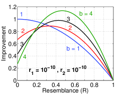
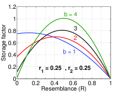
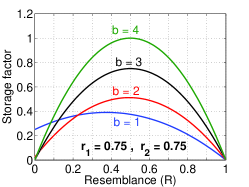
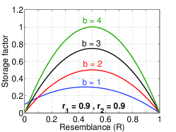
Figure 1: $B(b;R,r_{1},r_{2})$ in (15). The lower the better.

The ratio of storage factors, $\frac{B(b_{1};R,r_{1},r_{2})}{B(b_{2};R,r_{1},r_{2})}$, directly measures how much improvement using $b=b_{2}$ (e.g., $b_{2}=1$) can have over using $b=b_{1}$ (e.g., $b_{1}=64$ or 32).

Some algebraic manipulation yields the following Theorem.

Theorem 2

If $r_{1}=r_{2}$ and $b_{1}>b_{2}$, then

$$\frac{B(b_{1};R,r_{1},r_{2})}{B(b_{2};R,r_{1},r_{2})}=\frac{b_{1}}{b_{2}}\ \frac{A_{1,b_{1}}(1-R)+R}{A_{1,b_{2}}(1-R)+R}\ \frac{1-A_{1,b_{2}}}{1-A_{1,b_{1}}},$$ (16)

is a monotonically increasing function of $R\in[0,1]$.

If $R\rightarrow 1$ (which implies $r_{1}\rightarrow r_{2}$), then

$$\frac{B(b_{1};R,r_{1},r_{2})}{B(b_{2};R,r_{1},r_{2})}\rightarrow\frac{b_{1}}{b_{2}}\frac{1-A_{1,b_{2}}}{1-A_{1,b_{1}}}.$$ (17)

If $r_{1}=r_{2}$, $b_{2}=1$, $b_{1}\geq 32$ (hence we treat $A_{1,b}=0$), then

$$\frac{B(b_{1};R,r_{1},r_{2})}{B(1;R,r_{1},r_{2})}=b_{1}\frac{R}{R+1-r_{1}}$$ (18)

Proof:  We omit the proof due to its simplicity.$\Box$

Suppose the original minwise hashing used $b=64$ bits to store each sample, then the maximum improvement of the $b$-bit minwise hashing would be 64-fold, attained when $r_{1}=r_{2}=1$ and $R=1$, according to (18). In the least favorable situation, i.e., $r_{1},r_{2}\rightarrow 0$, the improvement will still be $\frac{64R}{R+1}$-fold, which is $\frac{64}{3}=21.3$-fold when $R=0.5$.

Figure 2 plots $\frac{B(32)}{B(b)}$, to directly visualize the relative improvement. The plots are, of course, consistent with what Theorem 2 would predict.

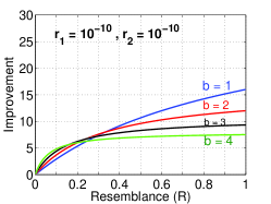
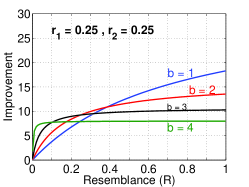
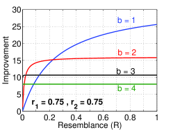
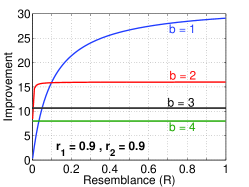
Figure 2: $\frac{B(32)}{B(b)}$, the relative storage improvement of using $b=1,2,3,4$ bits, compared to using $32$ bits.

3 Experiments

We conducted three experiments. The first two experiments were based on a set of 2633 words, extracted from a chuck of MSN Web pages. Our third experiment used a set of 10000 news articles crawled from the Web.

Our first experiment is a sanity check, to verify the correctness of the theory. That is, our proposed estimator $\hat{R}_{b}$, (12), is unbiased and its variance (the same as the mean square error (MSE)) follows the prediction by our formula in (14).

3.1 Experiment 1

For our first experiment, we selected 10 pairs of words to validate the theoretical estimator $\hat{R}_{M}$ and the variance formula $\text{Var}\left(\hat{R}_{M}\right)$, derived in in Sec. 2.1.

Table 1 summarizes the data and also provides the theoretical improvements $\frac{B(32)}{B(1)}$ and $\frac{B(64)}{B(1)}$. For each word, the data consist of the document IDs in which that word occurs. The words were selected to include highly frequent word pairs (e.g., “OF-AND”), highly rare word pairs (e.g., “GAMBIA-KIRIBATI”), highly unbalanced pairs (e.g., ”A-Test”), highly similar pairs (e.g, “KONG-HONG”), as well as word pairs that are not quite similar (e.g., “LOW-PAY”).

Table 1: Ten pairs of words used in the experiments for validating the estimator and theoretical variance (14). Since the variance is determined by $r_{1}$, $r_{2}$, and $R$, words were selected to ensure a good coverage of scenarios.

Word 1	Word 2	$r_{1}$	$r_{2}$	$R$	$\frac{B(32)}{B(1)}$	$\frac{B(64)}{B(1)}$
KONG	HONG	0.0145	0.0143	0.925	15.5	31.0
RIGHTS	RESERVED	0.187	0.172	0.877	16.6	32.2
OF	AND	0.570	0.554	0.771	20.4	40.8
GAMBIA	KIRIBATI	0.0031	0.0028	0.712	13.3	26.6
UNITED	STATES	0.062	0.061	0.591	12.4	24.8
SAN	FRANCISCO	0.049	0.025	0.476	10.7	21.4
CREDIT	CARD	0.046	0.041	0.285	7.3	14.6
TIME	JOB	0.189	0.05	0.128	4.3	8.6
LOW	PAY	0.045	0.043	0.112	3.4	6.8
A	TEST	0.596	0.035	0.052	3.1	6.2

We estimate the resemblance using the original minwise hashing estimator $\hat{R}_{M}$ and the $b$-bit version for $b=1,2,3$.

Figure 3 presents the estimation biases for selected 4 word pairs. Theoretically, the estimator $\hat{R}_{b}$ is unbiased. Figure 3 verifies this fact as the empirical biases are all very small and no systematic biases can be observed.

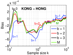
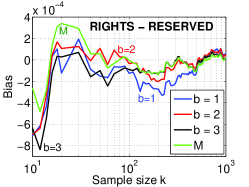
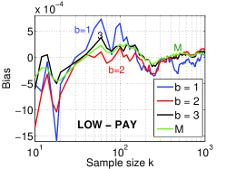
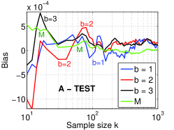
Figure 3: Biases, empirically estimated from 25000 simulations at each sample size $k$. “M” denotes the original minwise hashing.

Figure 4 plots the empirical mean square errors (MSE = variance + bias²) and the theoretical variances (in dashed lines), for all 10 word pairs. However, all dashed lines overlapped with the corresponding solid curves. This figure satisfactorily illustrates that the variance formula (14) is accurate and $\hat{R}_{b}$ is indeed unbiased (because MSE=variance).

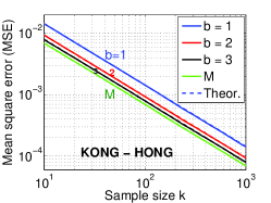
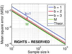
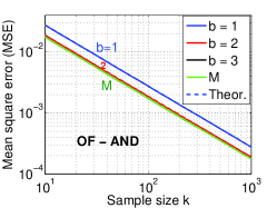
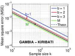
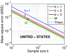
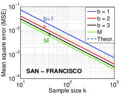
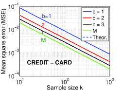
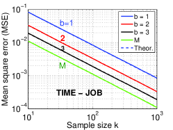
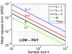
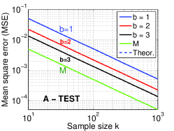
Figure 4: MSEs, empirically estimated from simulations. “M” denotes the original minwise hashing. “Theor.” denotes the theoretical variances of $Var(\hat{R}_{b})$ and $Var(\hat{R}_{M})$. Those dashed curves, however, are invisible because the empirical results overlapped the theoretical predictions. At the same sample size $k$, we always have $Var(\hat{R}_{1})>Var(\hat{R}_{2})>Var(\hat{R}_{3})>Var(\hat{R}_{M})$. However, $\hat{R}_{1}$ only requires 1 bit per sample while $\hat{R}_{2}$ requires 2 bits, etc.

3.2 Experiment 2

This section presents an experiment for finding pairs whose resemblance values $\geq R_{0}$. This experiment is in the same spirit as [3, 5]. We use all 2633 words (i.e., 3465028 pairs) as described in Experiment 1. We use both $\hat{R}_{M}$ and $\hat{R}_{b}$ ($b=1,2,3,4$) and then present the precision and recall curves, at different values of thresholds $R_{0}$ and sample sizes $k$.

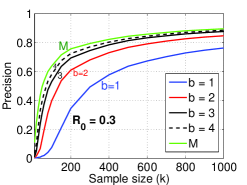
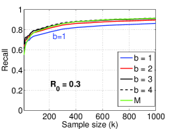
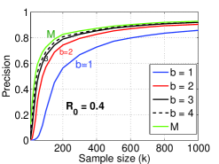
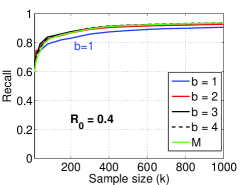
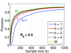
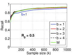
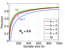
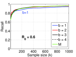
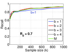
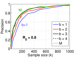
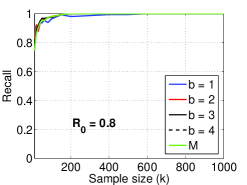
Figure 5: Precision & Recall, averaged over 700 repetitions. The task is to retrieve pairs with $R\geq R_{0}$.

Figure 5 presents the precision and recall curves. The recall curves (right panels) do not well differentiate $\hat{R}_{M}$ from $\hat{R}_{b}$ (unless $b=1$). The precision curves (left panel) show more clearly that using $b=1$ may result in lower precision values than $\hat{R}_{M}$ (especially when $R_{0}$ is small), at the same sample size $k$. When $b\geq 3$, $\hat{R}_{b}$ performs very similarly to $\hat{R}_{M}$.

We stored each sample for $\hat{R}_{M}$ using 32 bits, although in real applications, 64 bits may be needed[3, 5, 10]. Table 2 summarizes the relative improvements of $\hat{R}_{b}$ over $\hat{R}_{M}$, in terms of bits, for each threshold $R_{0}$. Not surprisingly, the results are quite consistent with Figure 2.

Table 2: Relative improvement (in space) of $\hat{R}_{b}$ (using $b$ bits per sample) over $\hat{R}_{M}$ (32 bits per sample). For precision = 0.7, 0.8, we find the required sample sizes (from Figure 5) for $\hat{R}_{M}$ and $\hat{R}_{b}$ and use them to estimate the required storage in bits. The values in the table are the ratios of the storage bits. For $b=1$ and threshold $R_{0}\geq 0.5$, the improvements are roughly $10\sim 18$-fold, consistent with the theoretical predictions in Figure 2.

$R_{0}$	Precision = $0.70$	Precision = $0.80$
	$b=1$   2     3     4	$b=1$   2     3     4
0.3	6.49   6.61   7.04   6.40	—-    7.96   7.58   6.58
0.4	7.86    8.65   7.48   6.50	8.63   8.36   7.71    6.91
0.5	9.52   9.23    7.98   7.24	11.1   9.85   8.22   7.39
0.6	11.5    10.3    8.35    7.10	13.9   10.2   8.07   7.28
0.7	13.4    12.2    9.24    7.20	14.5   12.3   8.91   7.39
0.8	17.6    12.5    9.96    7.76	18.2   12.8   9.90    8.08

3.3 Experiment 3

To illustrate the improvements by the use of b-bit minwise hashing on a real-life application, we conducted a duplicate detection experiment using a corpus of 10000 news documents (49995000 pairs). The dataset was crawled as part of the BLEWS project at Microsoft[12]. In the news domain, duplicate detection is an important problem as (e.g.) search engines must not serve up the same story multiple times and news stories (especially AP stories) are commonly copied with slight alterations/changes in bylines only.

In the experiments we computed the pairwise resemblances for all documents in the set; we present the data for retrieving document pairs with resemblance $R\geq R_{0}$ below.

We estimate the resemblances using $\hat{R}_{b}$ with $b=1$, 2, 4 bits, and the original minwise hashing (using 32 bits). Figure 6 presents the precision & recall curves. The recall values are all very high (mostly $>0.95$) and do not well differentiate various estimators.

The precision curves for $\hat{R}_{4}$ (using 4 bits per sample) and $\hat{R}_{M}$ (using 32 bits per sample) are almost indistinguishable, suggesting a 8-fold improvement in space using $b=4$.

When using $b=1$ or 2, the space improvements are normally around 10-fold to 15-fold, compared to $\hat{R}_{M}$, especially for achieving high precisions (e.g., $\geq 0.9$). This experiment again confirms the significant improvement of the $b$-bit minwise hashing using $b=1$ (or 2).

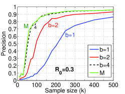
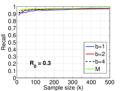
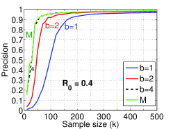
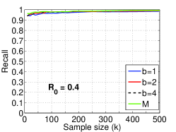
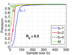
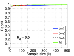
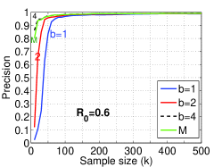
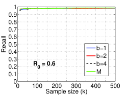
Figure 6: News Precision & Recall. The task is to retrieve news article pairs with $R\geq R_{0}$.

Note that in the context of (Web) document duplicate detection, in addition to shingling, a number of specialized hash-signatures have been proposed, which leverage properties of natural-language text (such as the placement of stopwords[25]). However, our approach is not aimed at any specific datesets, but is a general, domain-independent technique. Also, to the extent that other approaches rely on minwise hashing for signature computation, these may be combined with our techniques.

4 Discussion: Combining Bits for Enhancing Performance

Figure 1 and Figure 2 have shown that, for about $R\geq 0.4$, using $b=1$ always outperforms using $b>1$, even in the least favorable situation. This naturally leads to the conjecture that one may be able to further improve the performance using “$b<1$”, when $R$ is close to 1.

One simple approach to implement “$b<1$” is to combine two bits from two permutations.

Recall $e_{1,1,\pi}$ denotes the lowest bit of the hashed value under $\pi$. Theorem 1 has proved that

$$E_{1}=\mathbf{Pr}\left(e_{1,1,\pi}=e_{2,1,\pi}\right)=C_{1,1}+\left(1-C_{2,1}\right)R$$

Consider two permutations $\pi_{1}$ and $\pi_{2}$. We store

$$x_{1}=\text{XOR}(e_{1,1,\pi_{1}},\ e_{1,1,\pi_{2}}),\hskip 14.45377ptx_{2}=\text{XOR}(e_{2,1,\pi_{1}},\ e_{2,1,\pi_{2}})$$

Then $x_{1}=x_{2}$ either when $e_{1,1,\pi_{1}}=e_{2,1,\pi_{1}}$ and $e_{1,1,\pi_{2}}=e_{2,1,\pi_{2}}$, or, when $e_{1,1,\pi_{1}}\neq e_{2,1,\pi_{1}}$ and $e_{1,1,\pi_{2}}\neq e_{2,1,\pi_{2}}$. Thus

$$T=\mathbf{Pr}\left(x_{1}=x_{2}\right)=E_{1}^{2}+(1-E_{1})^{2},$$ (19)

which is a quadratic equation with solution

$$R=\frac{\sqrt{2T-1}+1-2C_{1,1}}{2-2C_{2,1}}.$$ (20)

We can estimate $T$ without bias as a binomial. However, the resultant estimator for $R$ will be biased, at small sample size $k$, due to the nonlinearity. We will recommend the following estimator

$$\hat{R}_{1/2}=\frac{\sqrt{\max\{2\hat{T}-1,0\}}+1-2C_{1,1}}{2-2C_{2,1}}.$$ (21)

The truncation $\max\{,0\}$ will introduce further bias; but it is necessary and is usually a good bias-variance trade-off.

We use $\hat{R}_{1/2}$ to indicate that two bits are combined into one. The asymptotic variance of $\hat{R}_{1/2}$ can be derived using the “delta method” in statistics:

$$\text{Var}\left(\hat{R}_{1/2}\right)=\frac{1}{k}\frac{T(1-T)}{4(1-C_{2,1})^{2}(2T-1)}+O\left(\frac{1}{k^{2}}\right).$$ (22)

One should keep in mind that, in order to generate $k$ samples for $\hat{R}_{1/2}$, we have to conduct $2\times k$ permutations. Of course, each sample is still stored using 1 bit, despite that we use “$b=1/2$” to denote this estimator.

Interestingly, as $R\rightarrow 1$, $\hat{R}_{1/2}$ does twice as well as $\hat{R}_{1}$:

$$\lim_{R\rightarrow 1}\frac{\text{Var}\left(\hat{R}_{1}\right)}{\text{Var}\left(\hat{R}_{1/2}\right)}=\lim_{R\rightarrow 1}\frac{2(1-2E_{1})^{2}}{(1-E_{1})^{2}+E_{1}^{2}}=2.$$ (23)

Recall, if $R=1$, then $r_{1}=r_{2}$, $C_{1,1}=C_{2,1}$, and $E_{1}=C_{1,1}+1-C_{2,1}=1$.

On the other hand, $\hat{R}_{1/2}$ may not be an ideal estimator when $R$ is not too large. For example, one can numerically show that (as $k\rightarrow\infty$)

$$\text{Var}\left(\hat{R}_{1}\right)<\text{Var}\left(\hat{R}_{1/2}\right),\hskip 14.45377pt\text{if}\ \ R<0.5774,\ r_{1},\ r_{2}\rightarrow 0$$

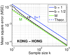
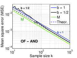
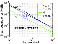
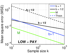
Figure 7: MSEs for comparing $\hat{R}_{1/2}$ with $\hat{R}_{1}$ and $\hat{R}_{M}$. Due to the bias, the theoretical variances $\text{Var}\left(\hat{R}_{1/2}\right)$, i.e., (22), deviate from the empirical MSEs when the sample size $k$ is not large.

Figure 7 plots the empirical MSEs for four word pairs in Experiment 1, for $\hat{R}_{1/2}$, $\hat{R}_{1}$, and $\hat{R}_{M}$:

• For the highly similar pair, “KONG-HONG,” $\hat{R}_{1/2}$ exhibits superb performance compared to $\hat{R}_{1}$.

• For the fairly similar pair, “OF-AND,” $\hat{R}_{1/2}$ is still considerably better.

• For “UNITED-STATES,” whose $R=0.591$, $\hat{R}_{1/2}$ performs similarly to $\hat{R}_{1}$.

• For “LOW-PAY,” whose $R=0.112$ only, the theoretical variance of $\hat{R}_{1/2}$ is very large. However, owing to the variance-bias trade-off, the empirical performance of $\hat{R}_{1/2}$ is not too bad.

In a summary, while the idea of combining two bits is interesting, it is mostly useful in applications which only care about pairs of very high similarities.

5 Conclusion

The minwise hashing technique has been widely used as a standard approach in information retrieval, for efficiently computing set similarity in massive data sets (e.g., duplicate detection). Prior studies commonly used $64$ or 40 bits to store each hashed value,

In this study, we propose the theoretical framework of $b$-bit minwise hashing, by only storing the lowest $b$ bits of each hashed value. We theoretically prove that, when the similarity is reasonably high (e.g., resemblance $\geq 0.5$), using $b=1$ bit per hashed value can, even in the worse case, gain a space improvement by $10.7\sim 16$-fold, compared to storing each hashed value using 32 bits. The improvement would be even more significant (e.g., at least $21.3\sim 32$-fold) if the original hashed values are stored using 64 bits.

We also discussed the idea of combining 2 bits from different hashed values, to further enhance the improvement, when the target similarity is very high.

Our proposed method is simple and requires only minimal modification to the original minwise hashing algorithm. We expect our method will be adopted in practice.

Appendix A Proof of Theorem 1

Consider two sets, $S_{1}$ and $S_{2}$,

$$S_{1},S_{2}\subseteq\Omega=\{0,1,2,...,D-1\},$$

$$f_{1}=|S_{1}|,\ f_{2}=|S_{2}|,\ a=|S_{1}\cap S_{2}|$$

We apply a random permutation $\pi$ on $S_{1}$ and $S_{2}$:

$$\pi:\Omega\longrightarrow\Omega.$$

Define the minimum values under $\pi$ to be $z_{1}$ and $z_{2}$:

$$z_{1}=\min\left(\pi\left(S_{1}\right)\right),\hskip 14.45377ptz_{2}=\min\left(\pi\left(S_{2}\right)\right).$$

Define $e_{1,i}=i$th lowest bit of $z_{1}$, and $e_{2,i}=i$th lowest bit of $z_{2}$. The task is to derive the analytical expression for

$$\mathbf{Pr}\left(\prod_{i=1}^{b}1\{e_{1,i}=e_{2,i}\}=1\right),$$

which can be decomposed to be

$$\mathbf{Pr}\left(\prod_{i=1}^{b}1\{e_{1,i}=e_{2,i}\}=1,\ z_{1}=z_{2}\right)$$

$$+ \mathbf{Pr}\left(\prod_{i=1}^{b}1\{e_{1,i}=e_{2,i}\}=1,\ z_{1}\neq z_{2}\right)$$

$$= \mathbf{Pr}\left(z_{1}=z_{2}\right)+\mathbf{Pr}\left(\prod_{i=1}^{b}1\{e_{1,i}=e_{2,i}\}=1,\ z_{1}\neq z_{2}\right)$$

$$= R+\mathbf{Pr}\left(\prod_{i=1}^{b}1\{e_{1,i}=e_{2,i}\}=1,\ z_{1}\neq z_{2}\right).$$

where $R=\frac{|S_{1}\cap S_{2}|}{|S_{1}\cup S_{2}|}=\mathbf{Pr}\left(z_{1}=z_{2}\right)$ is the resemblance.

When $b=1$, the task boils down to estimating

$$\mathbf{Pr}\left(e_{1,1}=e_{2,1},\ z_{1}\neq z_{2}\right)$$

$$= \sum_{i=0,2,4,...}\left\{\sum_{j\neq i,j=0,2,4,...}\mathbf{Pr}\left(z_{1}=i,z_{2}=j\right)\right\}$$

$$+ \sum_{i=1,3,5,...}\left\{\sum_{j\neq i,j=1,3,5,...}\mathbf{Pr}\left(z_{1}=i,z_{2}=j\right)\right\}.$$

Therefore, we need the following basic probability formula:

$$\mathbf{Pr}\left(z_{1}=i,\ z_{2}=j,\ i\neq j\right).$$

We will first start with

$$\mathbf{Pr}\left(z_{1}=i,\ z_{2}=j,\ i<j\right)=\frac{P_{1}+P_{2}}{P_{3}}$$

where

$$P_{3}=\binom{D}{a}\binom{D-a}{f_{1}-a}\binom{D-f_{1}}{f_{2}-a},$$

$$P_{1}=\binom{D-j-1}{a}\binom{D-j-1-a}{f_{2}-a-1}\binom{D-i-1-f_{2}}{f_{1}-a-1},$$

$$P_{2}=\binom{D-j-1}{a-1}\binom{D-j-a}{f_{2}-a}\binom{D-i-1-f_{2}}{f_{1}-a-1}.$$

The expressions for $P_{1}$, $P_{2}$, and $P_{3}$ can be understood by the experiment of randomly throwing $f_{1}+f_{2}-a$ balls into $D$ locations, labeled $0,1,2,...,D-1$. Those $f_{1}+f_{2}-a$ balls belong to three disjoint sets: $S_{1}-S_{1}\cap S_{2}$, $S_{2}-S_{1}\cap S_{2}$, and $S_{1}\cap S_{2}$. Without any restriction, the total number of combinations should be $P_{3}$.

To understand $P_{1}$ and $P_{3}$, we need to consider two cases:

1. The $j$th element is not in $S_{1}\cap S_{2}$ $\Longrightarrow P_{1}$.

2. The $j$th element is in $S_{1}\cap S_{2}$ $\Longrightarrow P_{2}$.
   

The next task is to simplify the expression for the probability $\mathbf{Pr}\left(z_{1}=i,\ z_{2}=j,\ i<j\right)$. After conducing expansions and cancelations, we obtain

$$\mathbf{Pr}\left(z_{1}=i,\ z_{2}=j,\ i<j\right)=\frac{P_{1}+P_{2}}{P_{3}}$$

$$= \frac{\left(\frac{1}{a}+\frac{1}{f_{2}-a}\right)\frac{(D-j-1)!(D-i-1-f_{2})!}{(a-1)!(f_{1}-a-1)(f_{2}-a-1)!(D-j-f_{2})!(D-i-f_{1}-f_{2}+a)!}}{\frac{D!}{a!(f_{1}-a)!(f_{2}-a)!(D-f_{1}-f_{2}+a)!}}$$

$$= \frac{f_{2}(f_{1}-a)(D-j-1)!(D-f_{2}-i-1)!(D-f_{1}-f_{2}+a)!}{D!(D-f_{2}-j)!(D-f_{1}-f_{2}+a-i)!}$$

$$= \frac{f_{2}(f_{1}-a)\prod_{t=0}^{j-i-2}(D-f_{2}-i-1-t)\prod_{t=0}^{i-1}(D-f_{1}-f_{2}+a-t}{\prod_{t=0}^{j}(D-t)}$$

$$= \frac{f_{2}}{D}\frac{f_{1}-a}{D-1}\prod_{t=0}^{j-i-2}\frac{D-f_{2}-i-1-t}{D-2-t}\prod_{t=0}^{i-1}\frac{D-f_{1}-f_{2}+a-t}{D+i-j-1-t}$$

For convenience, we introduce the following notation:

$$r_{1}=\frac{f_{1}}{D},\hskip 14.45377ptr_{2}=\frac{f_{2}}{D},\hskip 14.45377pts=\frac{a}{D}.$$

Also, we assume $D$ is large (which is always satisfied in practice). Thus, we can obtain a reasonable approximation:

$$\mathbf{Pr}\left(z_{1}=i,\ z_{2}=j,\ i<j\right)$$

$$= r_{2}(r_{1}-s)\left[1-r_{2}\right]^{j-i-1}\left[1-(r_{1}+r_{2}-s)\right]^{i}$$

Similarly, we obtain, for large $D$,

$$\mathbf{Pr}\left(z_{1}=i,\ z_{2}=j,\ i>j\right)$$

$$= r_{1}(r_{2}-s)\left[1-r_{1}\right]^{i-j-1}\left[1-(r_{1}+r_{2}-s)\right]^{j}$$

Now we have the tool to calculate the probability

$$\mathbf{Pr}\left(e_{1,1}=e_{2,1},\ z_{1}\neq z_{2}\right)$$

$$= \sum_{i=0,2,4,...}\left\{\sum_{j\neq i,j=0,2,4,...}\mathbf{Pr}\left(z_{1}=i,z_{2}=j\right)\right\}$$

$$+ \sum_{i=1,3,5,...}\left\{\sum_{j\neq i,j=1,3,5,...}\mathbf{Pr}\left(z_{1}=i,z_{2}=j\right)\right\}$$

For example, (again, assuming $D$ is large)

$$\mathbf{Pr}\left(z_{1}=0,z_{2}=2,4,6,...\right)$$

$$= r_{2}(r_{1}-s)\left([1-r_{2}]+[1-r_{2}]^{3}+[1-r_{2}]^{5}+...\right)$$

$$= r_{2}(r_{1}-s)\frac{1-r_{2}}{1-[1-r_{2}]^{2}}$$

$$\mathbf{Pr}\left(z_{1}=1,z_{2}=3,5,7,...\right)$$

$$= r_{2}(r_{1}-s)[1-(r_{1}+r_{2}-s)]\left([1-r_{2}]+[1-r_{2}]^{3}+[1-r_{2}]^{5}+...\right)$$

$$= r_{2}(r_{1}-s)[1-(r_{1}+r_{2}-s)]\frac{1-r_{2}}{1-[1-r_{2}]^{2}}.$$

Therefore,

$$\sum_{i=0,2,4,...}\left\{\sum_{i<j,j=0,2,4,...}\mathbf{Pr}\left(z_{1}=i,z_{2}=j\right)\right\}$$

$$+ \sum_{i=1,3,5,...}\left\{\sum_{i<j,j=1,3,5,...}\mathbf{Pr}\left(z_{1}=i,z_{2}=j\right)\right\}$$

$$= r_{2}(r_{1}-s)\frac{1-r_{2}}{1-[1-r_{2}]^{2}}\times$$

$$\left(1+[1-(r_{1}+r_{2}-s)]+[1-(r_{1}+r_{2}-s)]^{2}+...\right)$$

$$= r_{2}(r_{1}-s)\frac{1-r_{2}}{1-[1-r_{2}]^{2}}\frac{1}{r_{1}+r_{2}-s}.$$

By symmetry, we know

$$\sum_{j=0,2,4,...}\left\{\sum_{i>j,i=0,2,4,...}\mathbf{Pr}\left(z_{1}=i,z_{2}=j\right)\right\}$$

$$+ \sum_{j=1,3,5,...}\left\{\sum_{i>j,i=1,3,5,...}\mathbf{Pr}\left(z_{1}=i,z_{2}=j\right)\right\}$$

$$= r_{1}(r_{2}-s)\frac{1-r_{1}}{1-[1-r_{1}]^{2}}\frac{1}{r_{1}+r_{2}-s}.$$

Combining the probabilities, we obtain

$$\mathbf{Pr}\left(e_{1,1}=e_{2,1},\ z_{1}\neq z_{2}\right)$$

$$= \frac{r_{2}(1-r_{2})}{1-[1-r_{2}]^{2}}\frac{r_{1}-s}{r_{1}+r_{2}-s}+\frac{r_{1}(1-r_{1})}{1-[1-r_{1}]^{2}}\frac{r_{2}-s}{r_{1}+r_{2}-s}$$

$$= A_{1,1}\frac{r_{2}-s}{r_{1}+r_{2}-s}+A_{2,1}\frac{r_{1}-s}{r_{1}+r_{2}-s},$$

where

$$A_{1,b}=\frac{r_{1}\left[1-r_{1}\right]^{2^{b}-1}}{1-\left[1-r_{1}\right]^{2^{b}}},\hskip 14.45377ptA_{2,b}=\frac{r_{2}\left[1-r_{2}\right]^{2^{b}-1}}{1-\left[1-r_{2}\right]^{2^{b}}}.$$

Therefore, we can obtain the desired probability, for $b=1$,

$$\mathbf{Pr}\left(\prod_{i=1}^{b=1}1\{e_{1,i}=e_{2,i}\}=1\right)$$

$$= R+A_{1,1}\frac{r_{2}-s}{r_{1}+r_{2}-s}+A_{2,1}\frac{r_{1}-s}{r_{1}+r_{2}-s}$$

$$= R+A_{1,1}\frac{f_{2}-a}{f_{1}+f_{2}-a}+A_{2,1}\frac{f_{1}-a}{f_{1}+f_{2}-a}$$

$$= R+A_{1,1}\frac{f_{2}-\frac{R}{1+R}(f_{1}+f_{2})}{f_{1}+f_{2}-\frac{R}{1+R}(f_{1}+f_{2})}+A_{2,1}\frac{f_{1}-a}{f_{1}+f_{2}-a}$$

$$= R+A_{1,1}\frac{f_{2}-Rf_{1}}{f_{1}+f_{2}}+A_{2,1}\frac{f_{1}-Rf_{2}}{f_{1}+f_{2}}$$

$$= C_{1,1}+(1-C_{2,1})R$$

where

$$C_{1,b}=A_{1,b}\frac{r_{2}}{r_{1}+r_{2}}+A_{2,b}\frac{r_{1}}{r_{1}+r_{2}}$$

$$C_{2,b}=A_{1,b}\frac{r_{1}}{r_{1}+r_{2}}+A_{2,b}\frac{r_{2}}{r_{1}+r_{2}}.$$

To this end, we have proved the main result for $b=1$.

The proof for the general case, i.e., $b=2,3,...$, follows a similar procedure:

$$\mathbf{Pr}\left(\prod_{i=1}^{b}1\{e_{1,i}=e_{2,i}\}=1\right)$$

$$= R+A_{1,b}\frac{r_{2}-s}{r_{1}+r_{2}-s}+A_{2,b}\frac{r_{1}-s}{r_{1}+r_{2}-s}$$

$$= C_{1,b}+(1-C_{2,b})R.$$

The final task is to show some useful properties of $A_{1,b}$ (same for $A_{2,b}$). The first derivative of $A_{1,b}$ with respect to $b$ is

$$\frac{\partial A_{1,b}}{\partial b}= \frac{r_{1}[1-r_{1}]^{2^{b}-1}\log(1-r_{1})\log 2\left(1-[1-r_{1}]^{2^{b}}\right)}{\left(1-[1-r_{1}]^{2^{b}}\right)^{2}}$$

$$-\frac{-[1-r_{1}]^{2^{b}}\log(1-r_{1})\log 2\ r_{1}\left(1-[1-r_{1}]^{2^{b}-1}\right)}{\left(1-[1-r_{1}]^{2^{b}}\right)^{2}}$$

$$\leq 0\hskip 36.135pt(\text{Note that}\ \log(1-r_{1})\leq 0)$$

Thus, $A_{1,b}$ is a monotonically decreasing function of $b$.

Also,

$$\lim_{r_{1}\rightarrow 0}A_{1,b}=\lim_{r_{1}\rightarrow 0}\frac{\left[1-r_{1}\right]^{2^{b}-1}-r_{1}\left(2^{b}-1\right)[1-r_{1}]^{2^{b}-2}}{2^{b}[1-r_{1}]^{2^{b}-1}}=\frac{1}{2^{b}},$$

and

$$\frac{\partial A_{1,b}}{\partial r_{1}}= \frac{\left[1-r_{1}\right]^{2^{b}-1}-r_{1}\left(2^{b}-1\right)[1-r_{1}]^{2^{b}-2}}{\left(1-[1-r_{1}]^{2^{b}}\right)}$$

$$-\frac{2^{b}[1-r_{1}]^{2^{b}-1}r_{1}\left[1-r_{1}\right]^{2^{b}-1}}{\left(1-[1-r_{1}]^{2^{b}}\right)^{2}}$$

$$= \frac{[1-r_{1}]^{2^{b}-2}}{\left(1-[1-r_{1}]^{2^{b}}\right)^{2}}\left(1-2^{b}r_{1}-[1-r_{1}]^{2^{b}}\right)\leq 0.$$

Note that $(1-x)^{c}\geq 1-cx$, for $c\geq 1$ and $x\leq 1$.

Therefore $A_{1,b}$ is a monotonically decreasing function of $r_{1}$. We complete the whole proof.

References

- [1] Michael Bendersky and W. Bruce Croft. Finding text reuse on the web. In WSDM, pages 262–271, 2009.
- [2] Sergey Brin, James Davis, and Hector Garcia-Molina. Copy detection mechanisms for digital documents. In SIGMOD, pages 398–409, San Jose, CA, 1995.
- [3] Andrei Z. Broder. On the resemblance and containment of documents. In the Compression and Complexity of Sequences, pages 21–29, Positano, Italy, 1997.
- [4] Andrei Z. Broder, Moses Charikar, Alan M. Frieze, and Michael Mitzenmacher. Min-wise independent permutations. Journal of Computer Systems and Sciences, 60(3):630–659, 2000.
- [5] Andrei Z. Broder, Steven C. Glassman, Mark S. Manasse, and Geoffrey Zweig. Syntactic clustering of the web. In WWW, pages 1157 – 1166, Santa Clara, CA, 1997.
- [6] Gregory Buehrer and Kumar Chellapilla. A scalable pattern mining approach to web graph compression with communities. In WSDM, pages 95–106, Stanford, CA, 2008.
- [7] Moses S. Charikar. Similarity estimation techniques from rounding algorithms. In STOC, pages 380–388, Montreal, Quebec, Canada, 2002.
- [8] Flavio Chierichetti, Ravi Kumar, Silvio Lattanzi, Michael Mitzenmacher, Alessandro Panconesi, and Prabhakar Raghavan. On compressing social networks. In KDD, pages 219–228, Paris, France, 2009.
- [9] Yon Dourisboure, Filippo Geraci, and Marco Pellegrini. Extraction and classification of dense implicit communities in the web graph. ACM Trans. Web, 3(2):1–36, 2009.
- [10] Dennis Fetterly, Mark Manasse, Marc Najork, and Janet L. Wiener. A large-scale study of the evolution of web pages. In WWW, Budapest, Hungary, 2003.
- [11] George Forman, Kave Eshghi, and Jaap Suermondt. Efficient detection of large-scale redundancy in enterprise file systems. SIGOPS Oper. Syst. Rev., 43(1):84–91, 2009.
- [12] Michael Gamon, Sumit Basu, Dmitriy Belenko, Danyel Fisher, Matthew Hurst, and Arnd Christian König. BLEWS: Using blogs to provide context for news articles.
- [13] Sreenivas Gollapudi and Aneesh Sharma. An axiomatic approach for result diversification. In WWW, pages 381–390, Madrid, Spain, 2009.
- [14] Monika .R. Henzinge. Algorithmic challenges in web search engines. Internet Mathematics, 1(1):115–123, 2004.
- [15] Piotr Indyk. A small approximately min-wise independent family of hash functions. Journal of Algorithm, 38(1):84–90, 2001.
- [16] Toshiya Itoh, Yoshinori Takei, and Jun Tarui. On the sample size of k-restricted min-wise independent permutations and other k-wise distributions. In STOC, pages 710–718, San Diego, CA, 2003.
- [17] Nitin Jindal and Bing Liu. Opinion spam and analysis. In WSDM, pages 219–230, Palo Alto, California, USA, 2008.
- [18] Konstantinos Kalpakis and Shilang Tang. Collaborative data gathering in wireless sensor networks using measurement co-occurrence. Computer Communications, 31(10):1979–1992, 2008.
- [19] Eyal Kaplan, Moni Naor, and Omer Reingold. Derandomized constructions of k-wise (almost) independent permutations. Algorithmica, 55(1):113–133, 2009.
- [20] Ping Li and Kenneth W. Church. A sketch algorithm for estimating two-way and multi-way associations. Computational Linguistics, 33(3):305–354, 2007.
- [21] Ping Li, Kenneth W. Church, and Trevor J. Hastie. One sketch for all: Theory and applications of conditional random sampling. In NIPS, Vancouver, BC, Canada, 2009.
- [22] Ludmila, Kave Eshghi, Charles B. Morrey III, Joseph Tucek, and Alistair Veitch. Probabilistic frequent itemset mining in uncertain databases. In KDD, pages 1087–1096, Paris, France, 2009.
- [23] Marc Najork, Sreenivas Gollapudi, and Rina Panigrahy. Less is more: sampling the neighborhood graph makes salsa better and faster. In WSDM, pages 242–251, 2009.
- [24] Sandeep Pandey, Andrei Broder, Flavio Chierichetti, Vanja Josifovski, Ravi Kumar, and Sergei Vassilvitskii. Nearest-neighbor caching for content-match applications. In WWW, pages 441–450, Madrid, Spain, 2009.
- [25] Martin Theobald, Jonathan Siddharth, and Andreas Paepcke. Spotsigs: robust and efficient near duplicate detection in large web collections. In SIGIR, Singapore, 2008.
- [26] Tanguy Urvoy, Emmanuel Chauveau, Pascal Filoche, and Thomas Lavergne. Tracking web spam with html style similarities. ACM Trans. Web, 2(1):1–28, 2008.