Stochastic Analysis of Dimerization Systems

Abstract

The process of dimerization, in which two monomers bind to each other and form a dimer, is common in nature. This process can be modeled using rate equations, from which the average copy numbers of the reacting monomers and of the product dimers can then be obtained. However, the rate equations apply only when these copy numbers are large. In the limit of small copy numbers the system becomes dominated by fluctuations, which are not accounted for by the rate equations. In this limit one must use stochastic methods such as direct integration of the master equation or Monte Carlo simulations. These methods are computationally intensive and rarely succumb to analytical solutions. Here we use the recently introduced moment equations which provide a highly simplified stochastic treatment of the dimerization process. Using this approach, we obtain an analytical solution for the copy numbers and reaction rates both under steady state conditions and in the time-dependent case. We analyze three different dimerization processes: dimerization without dissociation, dimerization with dissociation and hetero-dimer formation. To validate the results we compare them with the results obtained from the master equation in the stochastic limit and with those obtained from the rate equations in the deterministic limit. Potential applications of the results in different physical contexts are discussed.

I Introduction

Dimerization is a common process in physical, chemical and biological systems. In this process, two identical units (monomers) bind to each other and form a dimer ($A+A\rightarrow A_{2}$). This is a special case of a more general reaction process (hetero-dimerization) of the form $A+B\rightarrow AB$. Dimerization may appear either as an isolated process or incorporated in a more complex reaction network. The modeling of dimerization systems is commonly done using rate equations, which incorporate the mean-field approximation. These equations describe the time evolution of the concentrations of the monomers and the dimers. Assuming that the system is spatially homogeneous, these concentrations can be expressed either in terms of the copy numbers per unit volume or in terms of the total copy number of each molecular species in the system. The rate equations are reliable when the copy numbers of the reacting monomers in the system are sufficiently large for the mean-field approximation to apply. However, when the copy numbers of the reacting monomers are low, the system becomes highly fluctuative, and the rate equations are no longer suitable. Therefore the analysis of dimerization processes under conditions of low copy numbers requires the use of stochastic methods vanKampen1981 ; Gardiner2004 . These methods include the direct integration of the master equation Biham2001 ; Green2001 , and Monte Carlo (MC) simulations Gillespie1976 ; Gillespie1977 ; Tielens1982 ; Newman1999 ; Charnley2001 . The master equation consists of coupled differential equations for the probabilities of all the possible microscopic states of the system. These equations are typically solved by numerical integration. However, in some simple cases, the steady state probabilities can be obtained by analytical methods Green2001 ; Biham2002 . The difficulty with the master equation is that it consists of a large number of equations, particularly if the dimerization process is a part of a larger network. This severely limits its usability for the analysis of complex reaction networks Stantcheva2002 ; Stantcheva2003 . Monte Carlo simulations provide a stochastic implementation of the master equation, following the actual temporal evolution of a single instance of the system. The mean copy numbers of the reactants and the reaction rates are obtained by averaging over an ensemble of such instances. In both methods, there is no closed form expression for the time dependence of the copy numbers and reaction rates.

Recently, a new method for the stochastic modeling of reaction networks was developed, which is based on moment equations Lipshtat2003 ; Barzel2007a ; Barzel2007 . The moment equations are much more efficient than the master equation. They consist of only one equation for each reactive species, one equation for each reaction rate, and in certain cases one equation for each product species. Thus, the number of moment equations that describe a given chemical network is comparable to the number of rate equations, which consist of one equation for each species. Moreover, unlike the rate equations, the moment equations are linear equations. In some cases, this feature enables to obtain an analytical solution for the time dependent concentrations.

In this paper, we apply the moment equations to the analysis of dimerization systems with fluctuations. These equations are accurate even in the limit of low copy numbers, where fluctuations are large and the rate equations fail. We show how to obtain an analytical solution for the time dependent concentrations of the reactant and product species as well as for the reaction rate. We identify and characterize the different dynamical regimes of the system as a function of the parameters. We examine the validity of our solution by comparison to the results obtained from the master equation. The analysis is performed for three variants of the system: dimerization, dimerization with dissociation and hetero-dimer formation.

The paper is organized as follows. In Sec. II we analyze the dimerization process using the moment equations and provide an analytical solution for the time-dependent concentrations. In Sec. III we extend the analysis to the case in which dimers may dissociate. In Sec. IV we generalize the analysis to the formation of hetero-dimers. The results are summarized and potential applications are discussed in Sec. V.

II Dimerization systems

Consider a system of molecules, denoted by $A$, which diffuse and react on a surface or in a liquid solution. Molecules are produced or added to the system at a rate $g$ (s^-1), and degrade at a rate $d_{1}$ (s^-1). When two molecules encounter each other they may bind and form the dimer $D$. The rate constant for the dimerization process is denoted by $a$ (s^-1). For simplicity, we assume that the product molecule, $D$, is non-reactive and undergoes degradation at a rate $d_{2}$ (s^-1). The chemical processes in this system can be described by

$$\varnothing\overset{g}{\longrightarrow}A$$

$$A\overset{d_{1}}{\longrightarrow}\varnothing$$

$$A+A\overset{a}{\longrightarrow}D$$

$$D\overset{d_{2}}{\longrightarrow}\varnothing.$$ (1)

II.1 Rate Equations

The dimerization system described above is characterized by the average copy number of the monomers, $\langle N_{A}\rangle$, and by the average copy number of the dimers, $\langle N_{D}\rangle$. Denoting the average dimerization rate by $\langle R\rangle$ (s^-1), the rate equations for this system take the form

$$\frac{d\langle N_{A}\rangle}{dt} = g-d_{1}\langle N_{A}\rangle-2\langle R\rangle$$

$$\frac{d\langle N_{D}\rangle}{dt} = -d_{2}\langle N_{D}\rangle+\langle R\rangle.$$ (2)

These equations include a term for each process which appears in Eq. (1). The factor of $2$ in the reaction term of the first equation accounts for the fact that the dimerization process removes two $A$ molecules, producing one dimer. The dimerization rate, $\langle R\rangle$, is proportional to the number of pairs of $A$ molecules in the system, $\langle N_{A}\rangle(\langle N_{A}\rangle-1)/2$, where the factor of $1/2$ is absorbed into the rate constant $a$. As long as the copy number of $A$ molecules is large, it can be approximated by

$$\langle R\rangle=a{\langle N_{A}\rangle}^{2}.$$ (3)

Eqs. (2) form a closed set of two non-linear differential equations. Their steady state solution is

$$\langle N_{A}\rangle^{\rm ss} = \frac{d_{1}}{4a}\left(-1+\sqrt{1+8\gamma}\right)$$

$$\langle N_{D}\rangle^{\rm ss} = \frac{d_{1}^{2}}{16ad_{2}}\left(-1+\sqrt{1+8\gamma}\right)^{2},$$ (4)

where $\gamma$ is the reaction strength parameter given by

$$\gamma=\frac{ag}{d_{1}^{2}}.$$ (5)

Two limits can be identified. In the limit where $\gamma\gg 1$, the steady state dimerization rate satisfies $\langle R\rangle^{\rm ss}\simeq g/2$, and the steady state dimer population is $\langle N_{D}\rangle^{\rm ss}\simeq g/2d_{2}$. This means that almost all the monomers that are generated end up in dimers and the monomer degradation process becomes irrelevant. Therefore, this limit is referred to as the reaction-dominated regime. The degradation-dominated limit is obtained when $\gamma\ll 1$. In this limit $\langle N_{A}\rangle^{\rm ss}\simeq g/d_{1}$, $\langle R\rangle^{\rm ss}\simeq ag^{2}/{d_{1}}^{2}=\gamma g$ and $\langle N_{D}\rangle^{\rm ss}\simeq ag^{2}/({d_{1}}^{2}d_{2})$, namely most of the monomers that are generated undergo degradation and only a small fraction end up in dimers.

The time-dependent solution for the population size of the $A$ molecules can be obtained from the first equation in Eqs. (2). The result is

$$\langle N_{A}\rangle=\langle N_{A}\rangle^{\rm ss}-\frac{1}{2a\tau}\left(1+Ce^{t/\tau}\right)^{-1},$$ (6)

where $\tau=1/\sqrt{d_{1}^{2}+8ag}$ is the relaxation time and the parameter $C$ is determined by the initial conditions. In the reaction-dominated regime, where $ag\gg d_{1}^{2}$, the relaxation time converges to $\tau\simeq 1/\sqrt{8ag}$. In the degradation-dominated regime, it approaches $\tau\simeq 1/d_{1}$.

The rate equation analysis is valid as long as the copy numbers of the reactive molecules are sufficiently large Lederhendler2008 . In the limit in which the copy number $\langle N_{A}\rangle$ of the monomers is reduced to order unity or less, the rate equations [Eqs. (2)] become unsuitable. This limit can be reached in two situations: when the monomer concentration is very low or when the volume of the system is very small. In the limit of low copy number of the monomers, the system becomes dominated by fluctuations which are not accounted for by the rate equations. A useful characterization of the system is given by the system-size parameter

$$N_{0}=\frac{g}{d_{1}},$$ (7)

which approximates the copy number of the monomers in case that the dimerization is suppressed. The parameter $N_{0}$ provides an upper limit for the monomer population size under steady state conditions. It can be used to characterize the dynamical regime of the system. In the limit where $N_{0}\gg 1$ the copy number of the monomers is typically large and the rate equations are reliable. However, when $N_{0}\lesssim 1$ the system may become dominated by fluctuations. In this regime, the rate equations fail to account for the population sizes and the dimerization rate. In Fig. 1 we present a schematic illustration of the parameter space in terms of $\gamma$ and $N_{0}$, identifying the four dynamical regimes.

II.2 Moment Equations

To obtain a more complete description of the dimerization process, which takes the fluctuations into account, we present the master equation approach. The dynamical variables of the master equation are the probabilities $P(N_{A},N_{D})$ of having a population of $N_{A}$ monomers and $N_{D}$ dimers in the system. The master equation for the dimerization system takes the form

$$\frac{dP(N_{A},N_{D})}{dt} = g[P(N_{A}-1,N_{D})-P(N_{A},N_{D})]$$

$$+ d_{1}[(N_{A}+1)P(N_{A}+1,N_{D})-N_{A}P(N_{A},N_{D})]$$

$$+ d_{2}[(N_{D}+1)P(N_{A},N_{D}+1)-N_{D}P(N_{A},N_{D})]$$

$$+ a[(N_{A}+2)(N_{A}+1)P(N_{A}+2,N_{D}-1)-N_{A}(N_{A}-1)P(N_{A},N_{D})].$$

The first term on the right hand side accounts for the addition or formation of $A$ molecules. The second and third terms account for the degradation of $A$ and $D$ molecules, respectively. The last term describes the reaction process, in which two $A$ molecules are annihilated and one $D$ molecule is formed. The dimerization rate is proportional to the number of pairs of $A$ molecules in the system, given by $N_{A}(N_{A}-1)/2$. Therefore, the dimerization rate can be expressed in terms of the moments of $P(N_{A},N_{D})$ as

$$\langle R\rangle=a\left(\langle{N_{A}}^{2}\rangle-\langle N_{A}\rangle\right),$$ (9)

where the moments are defined by

$$\langle N_{A}^{n}N_{D}^{m}\rangle=\sum_{\begin{subarray}{c}N_{A}=0\\ N_{D}=0\end{subarray}}^{\infty}{N_{A}^{n}N_{D}^{m}P(N_{A},N_{D})},$$ (10)

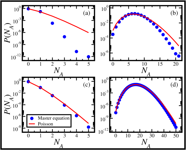
Figure 2: (color online) The steady state probability distribution $P(N_{A})$, as obtained from the master equation (circles) for (a) small degradation-dominated system; (b) small reaction-dominated system; (c) large degradation-dominated system and (d) large reaction-dominated system. For the degradation-dominated systems [(c) and (d)], $P(N_{A})$ can be fitted by a Poisson distribution (solid lines). For the reaction-dominated systems [(a) and (b)], $P(N_{A})$ significantly deviates from the Poisson distribution.

and $n$ and $m$ are integers. Note that in the stochastic formulation, the expression used for the dimerization rate, $\langle R\rangle$, is different than in the deterministic approach [Eq. (3)]. The two expressions are equal in case that $P(N_{A})$ is a Poisson distribution, for which the mean and the variance are equal. The master equation (II.2) for the dimerization system can be analytically solved to obtain the steady state probabilities $P(N_{A})$. This solution can be found at refs. Green2001 ; Biham2002 . However, an analytical solution for the time dependent case is currently not available. For dimerization systems in the degradation-dominated limit, the probability distribution $P(N_{A})$ approaches the Poisson distribution. However as $\gamma$ increases, and the system enters the reaction-dominated regime, $P(N_{A})$ becomes different from Poisson. In Fig. 2 we present the marginal probability distributions $P(N_{A})$ (circles) as obtained from the master equation for four choices of the parameters, each in one of the four regimes shown in Fig. 1. In the limit of $N_{0}\ll 1$ and $\gamma\gg 1$ (a) the system is in the reaction dominated regime (quadrant I in Fig. 1), and the results obtained from the master equation deviate from Poisson (solid lines). Here the parameters are $g=0.5$, $d_{1}=2$, $a=200$ and $d_{2}=10$ (s^-1). The distribution shown in (b), where $N_{0}\gg 1$ and $\gamma\gg 1$ (quadrant II in Fig. 1), also deviates from the Poisson distribution. Here the parameters are $g=100$, $d_{1}=1$, $a=1$ and $d_{2}=10$ (s^-1). In the limit of $N_{0}\ll 1$ and $\gamma\ll 1$ (c) the system is in the degradation-dominated regime (quadrant III in Fig. 1), and correspondingly $P(N_{A})$ coincides with the Poisson distribution. Here the parameters are $g=0.5$, $d_{1}=5$, $a=1$ and $d_{2}=10$ (s^-1). Finally, in (d) $N_{0}\gg 1$ and $\gamma\ll 1$ (quadrant IV in Fig. 1), the system is dominated by degradation and as before, the master equation results coincide with the Poisson distribution. Here the parameters are $g=10$, $d_{1}=1$, $a=5\times 10^{-3}$ and $d_{2}=10$ (s^-1).

In addition to the analytical solution mentioned above, the master equation [Eq. (II.2)] can also be integrated numerically using standard steppers such as the Runge Kutta method Acton1970 ; Press1992 . In numerical simulations, one has to truncate the master equation in order to keep the number of equations finite. This is achieved by setting upper cutoffs $N_{A}^{\rm max}$ and $N_{D}^{\rm max}$ on the numbers of $A$ and $D$ molecules, respectively. This truncation is valid if the probability for the number of molecules of each type to exceed the cutoff is vanishingly small.

The population sizes of the $A$ and $D$ molecules and the dimerization rate are expressed in terms of the first moments of $P(N_{A},N_{D})$ and one of its second moments, $\langle{N_{A}}^{2}\rangle$. Therefore, a closed set of equations for the time derivatives of these first and second moments could directly provide all the information needed in order to evaluate the population sizes and the dimerization rate Lipshtat2003 . Such equations can be obtained from the master equation using the identity

$$\frac{d\langle N_{A}^{n}N_{D}^{m}\rangle}{dt}=\sum_{\begin{subarray}{c}N_{A}=0\\ N_{D}=0\end{subarray}}^{\infty}{N_{A}^{n}N_{D}^{m}\dot{P}(N_{A},N_{D})}.$$ (11)

Inserting the time-derivative $\dot{P}(N_{A},N_{D})$ according to Eq. (II.2), one obtains the moment equations. The equations for the average copy numbers are

$$\frac{d\langle N_{A}\rangle}{dt} = g-d_{1}\langle N_{A}\rangle-2\langle R\rangle$$

$$\frac{d\langle N_{D}\rangle}{dt} = -d_{2}\langle N_{D}\rangle+\langle R\rangle,$$ (12)

while the equation for the dimerization rate is

$$\frac{d\langle R\rangle}{dt}=(2ag+4a^{2})\langle N_{A}\rangle+(10a-2d_{1})\langle R\rangle-4a^{2}\langle{N_{A}}^{3}\rangle.$$ (13)

Eqs. (12) have the same form as the rate equations (2). However the term for the dimerization rate, $\langle R\rangle$, as appears in the moment equations is different from the analogous term in the rate equations [Eq. (3)].

Eqs. (12), together with Eq. (13), are a set of coupled differential equations, which are linear in terms of the moments. Although we have written the equations only for the relevant first and second moments, the right hand side of Eq. (13) includes the third moment for which we have no equation. In order to close the set of equations one must express this third moment in terms of the first and second moments. Different expressions have been proposed. For example, in the context of birth-death processes the relation $\langle{N_{A}}^{3}\rangle=\langle{N_{A}}^{2}\rangle\langle N_{A}\rangle$ was used McQuarrie1967 . This choice makes the moment equations nonlinear, which might affect their stability. Another common choice is to assume that the third central moment is zero (which is exact for symmetric distributions) and use this relation to express the third moment in terms of the first and second moments Gomez-Uribe2007 . Here we use a different approach. We set up the closure condition by imposing a highly restrictive cutoff on the master equation. The cutoff is set at $N_{A}^{\rm max}=2$. This is the minimal cutoff that still enables the dimerization process to take place. Under this cutoff, one obtains the following relation between the first three moments Lipshtat2003

$$\langle{N_{A}}^{3}\rangle=3\langle{N_{A}}^{2}\rangle-2\langle N_{A}\rangle.$$ (14)

Using this result, one can bring the moment equations [Eqs. (12) - (13)] into a closed form:

$$\frac{d\langle N_{A}\rangle}{dt} = g-d_{1}\langle N_{A}\rangle-2\langle R\rangle$$

$$\frac{d\langle N_{D}\rangle}{dt} = -d_{2}\langle N_{D}\rangle+\langle R\rangle$$

$$\frac{d\langle R\rangle}{dt} = 2ag\langle N_{A}\rangle-2(d_{1}+a)\langle R\rangle.$$ (15)

Numerical integration of these equations provides all the required moments, from which the population sizes and the dimerization rate are obtained.

II.2.1 Steady State Analysis

The steady-state solution of the moment equations takes the form

$$\langle N_{A}\rangle^{\rm ss} = \frac{g(a+d_{1})}{2ag+d_{1}a+d_{1}^{2}}$$

$$\langle N_{D}\rangle^{\rm ss} = \frac{ag^{2}}{d_{2}(2ag+d_{1}a+d_{1}^{2})}$$

$$\langle R\rangle^{\rm ss} = \frac{ag^{2}}{2ag+d_{1}a+d_{1}^{2}}.$$ (16)

In the limit of very small copy numbers the approximation appearing in Eq. (14) is valid. Thus, in this limit the moment equations provide accurate results, both for the population sizes (first moments) and for the dimerization rate (involving a second moment). To evaluate the validity of the moment equations in the limit of large copy numbers, we compare Eqs. (16) with the solution of the rate equations (4), which is valid in this limit. Consider the large-system limit, where $N_{0}\gg 1$ [Eq. (7)]. In this limit, the common term in the denominators in Eqs. (16) approaches ${d_{1}}^{2}(2\gamma+1)$, where $\gamma$ is the reaction strength parameter, given by Eq. (5). Thus, in the degradation-dominated limit, where $\gamma\ll 1$, the steady state solution of the moment equations approaches

$$\langle N_{A}\rangle^{\rm ss} = \frac{g}{d_{1}}$$

$$\langle N_{D}\rangle^{\rm ss} = a\frac{g^{2}}{d_{2}{d_{1}}^{2}}$$

$$\langle R\rangle^{\rm ss} = a\frac{g^{2}}{{d_{1}}^{2}}.$$ (17)

Here we use the fact that in order to satisfy both the large-system limit ($N_{0}\gg 1$), and the degradation-dominated limit ($\gamma\ll 1$), one must also require $d_{1}\gg a$. The results appearing in Eqs. (17) are consistent with the results of the rate equations in this limit. We conclude that the moment equations are also reliable for large populations under the condition that the system is in the degradation-dominated regime. To test the results of the moment equations for large systems in the reaction-dominated regime we examine the case of $\gamma\gg 1$. Here Eqs. (16) are reduced to

$$\langle N_{A}\rangle^{\rm ss} = \frac{a+d_{1}}{2a}$$

$$\langle N_{D}\rangle^{\rm ss} = \frac{g}{2d_{2}}$$

$$\langle R\rangle^{\rm ss} = \frac{g}{2}.$$ (18)

In this limit, the monomer copy number $\langle N_{A}\rangle^{\rm ss}$, obtained from the moment equations, does not match the rate equation result. Nevertheless, the results for the dimer population size, $\langle N_{D}\rangle^{\rm ss}$, and for the dimerization rate $\langle R\rangle^{\rm ss}$, do converge to the results obtained from the rate equations.

We thus conclude that the accuracy of the moment equations is maintained well beyond the small system limit. The equations provide accurate results for the dimer copy number, $\langle N_{D}\rangle^{\rm ss}$, and for the dimerization rate, $\langle R\rangle^{\rm ss}$, for both small and large systems. As for the monomer copy number, the moment equations provide an accurate description in all limits, except for the limit where both $N_{0}\gg 1$ and $\gamma\gg 1$ (quadrant II in Fig. 1). In Table 1 we present a characterization of the different dynamical regimes and the applicability of the moment equations for the evaluation of the copy numbers and the dimerization rate in each regime.

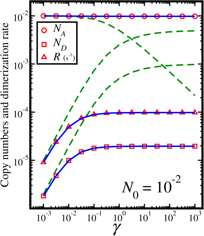
Figure 3: (color online) The average monomer copy number, $\langle N_{A}\rangle^{\rm ss}$ (circles), the average dimer copy number, $\langle N_{D}\rangle^{\rm ss}$ (squares) and the dimerization rate, $\langle R\rangle^{\rm ss}$ (triangles), versus the reaction strength parameter, $\gamma$, as obtained from the moment equations under steady state conditions. The parameters used here satisfy the small system limit, namely $N_{0}=10^{-2}$. The moment equation results are in perfect agreement with the results obtained from the master equation (solid lines). However, the rate equation results (dashed lines) show significant deviations. This is because in the limit of small monomer copy number the system is dominated by fluctuations, which are not accounted for by the rate equations. Note that $\langle N_{A}\rangle^{\rm ss}$ and $\langle N_{D}\rangle^{\rm ss}$ are dimensionless while $\langle R\rangle^{\rm ss}$ is units of s^-1.

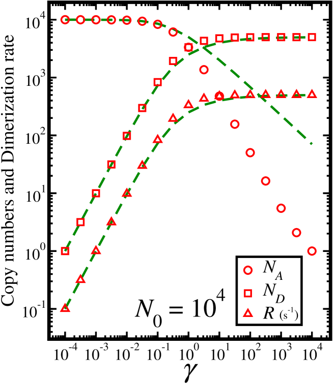
Figure 4: (color online) The average monomer copy number, $\langle N_{A}\rangle^{\rm ss}$ (circles), the average dimer copy number, $\langle N_{D}\rangle^{\rm ss}$ (squares) and the dimerization rate, $\langle R\rangle^{\rm ss}$ (triangles) versus the reaction strength parameter, $\gamma$, as obtained from the moment equations under steady state conditions. The parameters used here satisfy the large system limit, namely $N_{0}=10^{4}$. In this limit the rate equations (dashed lines) are reliable. The moment equation results are in agreement with the results obtained from the rate equations for the dimer copy number and its production rate. This is in spite of the fact that the copy numbers are large, far beyond the conditions for which the moment equations are designed. For the monomer copy number, the moment equations deviate in the reaction-dominated limit ($\gamma>1$). Slight deviations in the results for $\langle N_{D}\rangle^{\rm ss}$ and $\langle R\rangle^{\rm ss}$ appear around $\gamma\simeq 1$, where the crossover from the degradation-dominated regime to the reaction-dominated regime takes place.

In Fig. 3 we present the monomer copy number $\langle N_{A}\rangle^{\rm ss}$ (circles), the dimer copy number $\langle N_{D}\rangle^{\rm ss}$ (squares) and the dimerization rate $\langle R\rangle^{\rm ss}$ (triangles), as obtained from the moment equations, versus the reaction strength parameter, $\gamma$. The rate constants are $g=0.01$, $d_{1}=1$ and $d_{2}=5$ (s^-1). The reaction rate, $a$, is varied. These parameters satisfy the small-system limit $N_{0}\ll 1$. The moment equation results are in excellent agreement with those obtained from the master equation (solid lines). However, since the populations are small, the results of the rate equations show deviations (dashed lines). In Fig. 4 we present $\langle N_{A}\rangle^{\rm ss}$ (circles), $\langle N_{D}\rangle^{\rm ss}$ (squares) and $\langle R\rangle^{\rm ss}$ (triangles), as obtained from the moment equations, versus the reaction strength parameter, $\gamma$. Here the rate constants are $g=10^{3}$, $d_{1}=0.1$ and $d_{2}=0.1$ (s^-1). As before, the reaction rate, $a$, is varied. These parameters satisfy the large-system limit $N_{0}\gg 1$, and thus the rate equation results (dashed lines) are accurate. Although the populations are large for the entire parameter range displayed, the results of the moment equations are in excellent agreement with those obtained from the rate equations. The only deviation appears in the results for the monomer population in the limit $\gamma\gg 1$. For the parameters used in this simulation it was impractical to simulate the master equation.

In any chemical reaction it is important to characterize the extent to which fluctuations are significant. From the master equation, one can evaluate the fluctuation level in the monomer copy number, given by the variance

$$\sigma^{2}=\langle{N_{A}}^{2}\rangle-\langle N_{A}\rangle^{2},$$ (19)

where $\sigma$ is the standard deviation. The problem is that the expression for $\sigma$ includes the first moment $\langle N_{A}\rangle$, which is not always accurately accounted for by the moment equations. However, when the copy number is sufficiently large, the rate equations apply, and thus one can extract the value of $\langle N_{A}\rangle^{2}$ in this limit from the rate equations. On the other hand, the moment equations account correctly for the second moment $\langle{N_{A}}^{2}\rangle$ by $\langle{N_{A}}^{2}\rangle=\langle R\rangle/a+\langle N_{A}\rangle$. Using this relation, the result at steady state is

$$\sigma^{2} = \left\{\begin{array}[]{ccccr}\frac{g\left[d_{1}^{3}+a^{2}(d_{1}+g)+a(2d_{1}^{2}+d_{1}g+2g^{2})\right]}{\left(2ag+ad_{1}+d_{1}^{2}\right)^{2}}&&{\rm for}&&N_{0}\leq 1\\ \\ \frac{g(g+d_{1}+a)}{2ag+ad_{1}+d_{1}^{2}}-\frac{d_{1}^{2}}{16a}\left(-1+\sqrt{1+8\gamma}\right)^{2}&&{\rm for}&&N_{0}>1.\end{array}\right.$$ (23)

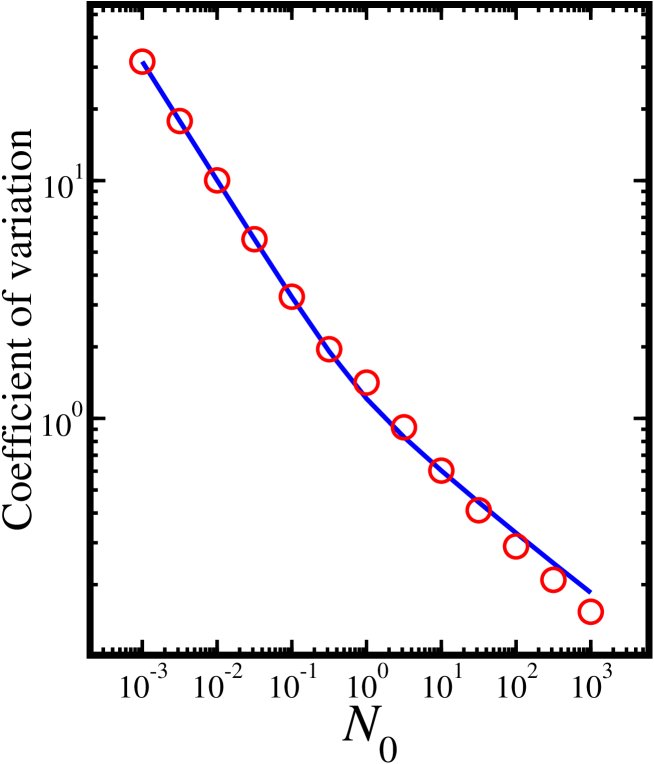
Figure 5: (color online) The coefficient of variation of the monomer copy number, $\sigma/\langle N_{A}\rangle^{\rm ss}$, versus the system size parameter $N_{0}$ (circles), as obtained from Eq. (23). As the average population size increases, $\sigma$ becomes smaller than $\langle N_{A}\rangle^{\rm ss}$. For $N_{0}<1$ the results are in perfect agreement with those obtained from the master equation (solid line). For $N_{0}>1$, where the expression in Eq. (23) combines results obtained from the moment equations and the rate equations, a slight deviation emerges. Nevertheless, Eq. (23) is shown to provide a good approximation for $\sigma$.

In Fig. 5 we present the coefficient of variation $\sigma/\langle N_{A}\rangle^{\rm ss}$ (circles), as obtained from Eq. (23) versus the system size parameter $N_{0}$. The parameters are $d_{1}=1$, $a=1$, $d_{2}=5$ (s^-1) and $g$ is varied. Here $\langle N_{A}\rangle^{\rm ss}$ was extracted from the moment equations for $N_{0}\leq 1$, and from the rate equations for $N_{0}>1$. In the small-system limit ($N_{0}\ll 1$), the average fluctuation becomes much larger than $\langle N_{A}\rangle^{\rm ss}$. The system is thus dominated by fluctuations. As the system size increases, $\sigma$ becomes small with respect to $\langle N_{A}\rangle^{\rm ss}$, implying that the system enters the deterministic regime. In order to validate our results, we compare them with results obtained from the master equation (solid line). For $N_{0}<1$ the agreement is perfect, as in this limit the moment equations are expected to be accurate. A slight deviation appears for $N_{0}>1$, where $\sigma$ is constructed by combining results obtained from the moment equations and from the rate equations. In both limits, Eq. (23) is found to provide a good approximation for the fluctuation level of the system.

II.2.2 Time-Dependent Solution

The time dependent solution for $\langle N_{A}\rangle$ can be obtained by solving the two coupled equations for $\langle N_{A}\rangle$ and for $\langle R\rangle$ in Eqs. (15). The equation for $\langle N_{D}\rangle$ receives input from these two equations. However, the dimers are the final products of this network and $\langle N_{D}\rangle$ has no effect on $\langle N_{A}\rangle$ and $\langle R\rangle$. Thus the equations for $\langle N_{A}\rangle$ and $\langle R\rangle$ can be decoupled from the equation for $\langle N_{D}\rangle$. One obtains a set of two coupled linear differential equations of the form

$$\dot{\vec{N}}={\bf M}\vec{N}+\vec{b},$$ (24)

where $\vec{N}=(\langle N_{A}\rangle,\langle R\rangle)$, $\vec{b}=(g,0)$ and the matrix ${\bf M}$ is

$${\bf M}=\left(\begin{array}[]{cc}-d_{1}&-2\\ 2ag&-2(d_{1}+a)\end{array}\right).$$ (27)

The two eigenvectors of the matrix ${\bf M}$ are given by

$$\vec{v}_{1}=\left(\begin{array}[]{c}\frac{2a+d_{1}-\omega}{4ag}\\ 1\end{array}\right); \vec{v}_{2}=\left(\begin{array}[]{c}\frac{2a+d_{1}+\omega}{4ag}\\ 1\end{array}\right),$$ (32)

where $\omega=\sqrt{4a^{2}+d_{1}^{2}+4ad_{1}-16ag}$. The corresponding eigenvalues are

$$-\frac{1}{\tau_{1}}=\frac{1}{2}(-2a-3d_{1}-\omega); -\frac{1}{\tau_{2}}=\frac{1}{2}(-2a-3d_{1}+\omega).$$ (33)

Using the matrix ${\bf Q}=(\vec{v}_{1},\vec{v}_{2})$, one can write Eq. (24) as

$${\bf Q}^{-1}\dot{\vec{N}}={\bf Q}^{-1}{\bf M}{\bf Q}{\bf Q}^{-1}\vec{N}+{\bf Q}^{-1}\vec{b}.$$ (34)

The result is a set of two un-coupled differential equations of the form

$$\dot{\vec{f}} = \left(\begin{array}[]{cc}-\frac{1}{\tau_{1}}&0\\ 0&-\frac{1}{\tau_{2}}\end{array}\right)\vec{f}+\vec{k},$$ (37)

where $\vec{f}={\bf Q}^{-1}\vec{N}$ and $\vec{k}={\bf Q}^{-1}\vec{b}$. The solution of Eq. (37) is

$$\vec{f}(t) = \left(\begin{array}[]{c}k_{1}\tau_{1}+C_{1}e^{-{t}/{\tau_{1}}}\\ k_{2}\tau_{1}+C_{2}e^{-{t}/{\tau_{2}}}\end{array}\right),$$ (40)

where $C_{1}$ and $C_{2}$ are arbitrary constants. Multiplying Eq. (40) from the left hand side by the matrix ${\bf Q}$ one obtains the time dependent solution of Eq. (24), which is

$$\langle N_{A}\rangle = \frac{g(a+d_{1})}{2ag+ad_{1}+d_{1}^{2}}+{\bf Q}_{1,1}C_{1}e^{-{t}/{\tau_{1}}}+{\bf Q}_{1,2}C_{2}e^{-{t}/{\tau_{2}}}$$

$$\langle R\rangle = \frac{ag^{2}}{2ag+ad_{1}+d_{1}^{2}}+{\bf Q}_{2,1}C_{1}e^{-{t}/{\tau_{1}}}+{\bf Q}_{2,2}C_{2}e^{-{t}/{\tau_{2}}}.$$ (41)

The first terms on the right hand side of Eqs. (41) are the steady state solutions $\langle N_{A}\rangle^{\rm ss}$ and $\langle R\rangle^{\rm ss}$ as they appear in Eqs. (16). The second and third terms represent the time-dependent parts of $\langle N_{A}\rangle$ and $\langle R\rangle$. These terms exhibit an exponential decay with two characteristic relaxation times, $\tau_{1}$ and $\tau_{2}$. Practically, since $\tau_{1}<\tau_{2}$, the effective relaxation time for the monomers is $\tau_{A}=\tau_{2}$.

In the limit of small copy numbers, where $N_{0}\ll 1$, Eqs. (41) account correctly for the copy numbers and for the reaction rates. In this limit (where $g\ll d_{1}$), one obtains $\tau_{A}\simeq 1/d_{1}$. In the limit of large copy numbers, where $N_{0}\gg 1$, one has to distinguish between degradation-dominated and reaction-dominated systems. Consider a degradation-dominated system, where $N_{0}\gg 1$ and $\gamma\ll 1$. These two conditions require that $d_{1}\gg a$. As before, the effective relaxation time is approximated by $\tau_{A}\simeq 1/d_{1}$. This result is consistent with the results of the rate equations in this regime [Eq. (6)]. A peculiar result arises in the reaction-dominated regime, in the limit of large populations. In this limit $\omega\simeq\sqrt{4a^{2}-16ag}$. For $a<4g$ the parameter $\omega$ becomes a purely imaginary number. This result leads to spurious oscillations in the solution presented in Eqs. (41). As shown for the steady state solution [Eq. (16)], the moment equations consistently fail in the limit of reaction-dominated systems with large copy numbers. To obtain the relaxation time in this limit, one can rely on the results obtained from the rate equations, which give $\tau_{A}\simeq 1/\sqrt{8ag}$. The relaxation times in all the different limits are summarized in Table 2.

Finally, we refer to the time evolution of the dimer population $\langle N_{D}\rangle$. The equation for $\langle N_{D}\rangle$ is the second equation in Eqs. (15), where $\langle R\rangle$ is to be taken from Eqs. (41). The solution of this equation takes the form

$$\langle N_{D}\rangle=\langle N_{D}\rangle^{\rm ss}+\tilde{C}_{1}e^{-{t}/{\tau_{1}}}+\tilde{C}_{2}e^{-{t}/{\tau_{2}}}+C_{3}e^{-{t}/{\tau_{3}}},$$ (42)

where $\langle N_{D}\rangle^{\rm ss}$ is taken from Eqs. (16), $\tilde{C}_{i}={\bf Q}_{2,i}C_{i}/[d_{2}-(1/\tau_{i})]$, $\tau_{3}=1/d_{2}$ and $C_{3}$ is an arbitrary constant. The effective relaxation time for the copy number of the dimer product depends on the value of $\tau_{3}$. If $\tau_{3}<\tau_{A}$, the copy number of the dimers relaxes rapidly. Thus, the time required for the dimers to reach steady state is determined by the monomer relaxation time, namely $\tau_{D}\simeq\tau_{A}$. In the opposite case, where $\tau_{3}>\tau_{A}$, the monomer population reaches steady state quickly, and the production rate of the dimers acts in effect as a constant generation rate. Correspondingly, the relaxation time for $\langle N_{D}\rangle$ in this limit is approximated by $\tau_{D}\simeq 1/d_{2}$ (Table 2).

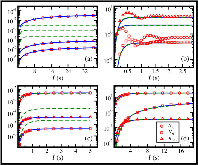
Figure 6: (color online) The time dependence of $\langle N_{A}\rangle$ (circles), $\langle N_{D}\rangle$ (squares) and $\langle R\rangle$ (triangles), as obtained from the moment equations. Four different limits are observed. In the limit where $N_{0}\ll 1$ and $\gamma\gg 1$ (a) the moment equations are in perfect agreement with the master equation. In this limit, the rate equations fail to account both for the steady state copy numbers and for the relaxation time. According to the rate equations, the relaxation time is $\tau\simeq 1/\sqrt{8ag}$, while according to the moment equations it is $\tau\simeq 1/d_{1}$, in agreement with the master equation. In the limit where $N_{0}\gg 1$ and $\gamma\gg 1$ (b), the rate equations and the master equation are in good agreement. In this limit the moment equations fail to produce the correct time dependent solution, as they predict an oscillatory convergence towards steady state. Note, however, that even in this limit, the moment equations do provide correct results for the steady state values of $\langle N_{D}\rangle$ and $\langle R\rangle$. In the limit where $N_{0}\ll 1$ and $\gamma\ll 1$ (c), the moment equations are in perfect agreement with the master equation (solid lines). The rate equations (dashed lines), which do not account for fluctuations, fail in this limit. The limit where $N_{0}\gg 1$ and $\gamma\ll 1$ is shown in (d). Although the copy numbers are large in this limit, the moment equations are still in perfect agreement with the master equation. Not surprisingly, the rate equations also apply.

In Fig. 6(a) we present the time evolution of $\langle N_{A}\rangle$ (circles) $\langle N_{D}\rangle$ (squares) and $\langle R\rangle$ (triangles), as obtained from the moment equations. The parameters are $g=2\times 10^{-3}$, $d_{1}=0.05$, $a=100$ and $d_{2}=5$ (s^-1). These parameters correspond to the small system limit and to the reaction-dominated regime (quadrant I in Fig. 1). The moment equations (symbols) are in perfect agreement with the master equation (solid lines). The rate equations (dashed lines) deviate from the stochastic results both in evaluating the steady state values of $\langle N_{A}\rangle$, $\langle N_{D}\rangle$ and $\langle R\rangle$, and in predicting the relaxation times of $\langle N_{A}\rangle$ and $\langle R\rangle$. According to the rate equations, this relaxation time should be $\tau_{A}\simeq 1/\sqrt{8ag}\simeq 0.8$ (s), while according to the stochastic description $\tau_{A}\simeq 1/d_{1}\simeq 20$ (s). In Fig. 6(b) we present results for a system in the large population limit and in the regime of reaction-dominated kinetics (quadrant II in Fig. 1). Here the parameters are $g=10$, $d_{1}=0.5$, $a=1$ and $d_{2}=10$ (s^-1). Under these conditions the moment equations fail to produce the correct time transient, and give rise to an oscillatory solution (symbols). In this regime the results obtained from the rate equations (dashed lines) are accurate and coincide with the master equation results (solid lines). Note that even in this case the moment equations provide the correct values for the dimer production rate, $\langle R\rangle$, and for the dimer population, $\langle N_{D}\rangle$, under steady state conditions. In Fig. 6(c) the parameters are $g=0.01$, $d_{1}=2$, $a=10$ and $d_{2}=10$ (s^-1). These parameters satisfy the small system limit and are in the kinetic regime dominated by degradation (quadrant III in Fig. 1). The results are in perfect agreement with those obtained from the master equation (solid lines). However, the rate equations (dashed lines), although displaying similar relaxation times, show significant deviations in the steady state values of $\langle N_{D}\rangle$ and $\langle R\rangle$. In Fig. 6(d) we present results for the case of a large system, where the parameters are $g=10$, $d_{1}=0.5$, $a=10^{-3}$ and $d_{2}=0.05$ (s^-1). These parameters correspond to a system in the degradation-dominated regime (quadrant IV in Fig. 1). Although in this system the copy numbers are large, the results obtained from the moment equations (symbols) are in perfect agreement with those obtained from the master equation (solid lines) and from the rate equations (dashed lines). Here the relaxation time for the monomer population is $\tau_{A}\simeq 1/d_{1}$ and for the dimer population it is $\tau_{D}\simeq 1/d_{2}$.

III Dimerization-Dissociation Systems

To generalize the discussion of the previous Section we now consider the case where the dimer product $D$ may undergo dissociation into two monomers, at a rate $u$ (s^-1). The chemical processes in this system are thus

$$\varnothing\overset{g}{\longrightarrow}A$$

$$A\overset{d_{1}}{\longrightarrow}\varnothing$$

$$A+A\overset{a}{\longrightarrow}D$$

$$D\overset{d_{2}}{\longrightarrow}\varnothing$$

$$D\overset{u}{\longrightarrow}A+A.$$ (43)

III.1 Rate Equations

The rate equations for this reaction take the form

$$\frac{d\langle N_{A}\rangle}{dt} = g-d_{1}\langle N_{A}\rangle-2\langle R\rangle+2u\langle N_{D}\rangle$$

$$\frac{d\langle N_{D}\rangle}{dt} = -(d_{2}+u)\langle N_{D}\rangle+\langle R\rangle,$$ (44)

where $\langle R\rangle=a\langle N_{A}\rangle^{2}$. These equations are similar to Eqs. (2), except for the $u$ terms which account for the dissociation. We define the effective reaction rate constant as $a_{\rm eff}=a[d_{2}/(u+d_{2})]$ such that the effective dimerization rate is $\langle R\rangle_{\rm eff}=a_{\rm eff}\langle N_{A}\rangle^{2}$. Under steady state conditions, Eqs. (44) can be written as

$$g-d_{1}\langle N_{A}\rangle-2\langle R\rangle_{\rm eff} = 0$$

$$\langle R\rangle_{\rm eff}-d_{2}\langle N_{D}\rangle = 0.$$ (45)

They take the same form as Eqs. (2), for dimerization without dissociation, under steady state conditions. The steady state solution for these equations is

$$\langle N_{A}\rangle^{\rm ss} = \frac{d_{1}}{4a_{\rm eff}}\left(-1+\sqrt{1+8\gamma_{\rm eff}}\right)$$

$$\langle N_{D}\rangle^{\rm ss} = \frac{d_{1}^{2}}{16a_{\rm eff}d_{2}}\left(-1+\sqrt{1+8\gamma_{\rm eff}}\right)^{2},$$ (46)

where

$$\gamma_{\rm eff}=\frac{ga_{\rm eff}}{d_{1}^{2}}$$ (47)

is the effective reaction strength parameter. In the limit where $d_{2}\gg u$, most dimers undergo degradation. The dissociation process is suppressed, and the effective reaction rate constant is $a_{\rm eff}\simeq a$, namely the solution approaches that of dimerization without dissociation. In the limit where $d_{2}\ll u$, most of the produced dimers end up dissociating into monomers, and correspondingly $a_{\rm eff}\rightarrow 0$. In this limit, the dimerization and dissociation processes reach a balance. The effective dimerization rate vanishes and $\langle N_{A}\rangle^{\rm ss}\simeq g/d_{1}$.

III.2 Moment Equations

In order to conduct a stochastic analysis we present the master equation for the dimerization-dissociation system, which takes the form

$$\frac{dP(N_{A},N_{D})}{dt} = g[P(N_{A}-1,N_{D})-P(N_{A},N_{D})]$$ (48)

$$+ d_{1}[(N_{A}+1)P(N_{A}+1,N_{D})-N_{A}P(N_{A},N_{D})]$$

$$+ d_{2}[(N_{D}+1)P(N_{A},N_{D}+1)-N_{D}P(N_{A},N_{D})]$$

$$+ a[(N_{A}+2)(N_{A}+1)P(N_{A}+2,N_{D}-1)-N_{A}(N_{A}-1)P(N_{A},N_{D})]$$

$$+ u[(N_{D}+1)P(N_{A}-2,N_{D}+1)-N_{D}P(N_{A},N_{D})].$$

This equation resembles Eq. (II.2), except for the last term which accounts for the dissociation process. The master equation can be solved numerically by imposing suitable cutoffs, $N_{A}^{\rm max}$ and $N_{D}^{\rm max}$. However an analytical solution is currently unavailable. To obtain a much simpler stochastic description of this system we refer to the moment equations. Following the same steps as in the previous Section, we impose the minimal cutoffs on the master equation, that enable all the required processes to take place. More specifically, we choose $N_{A}^{\rm max}=2$ in order to enable the dimerization. We do not limit the copy number of the dimer, $N_{D}$. However, we do not allow $N_{A}\neq 0$ and $N_{D}\neq 0$ simultaneously, because $A$ and $D$ molecules do not react with each other. These cutoffs reproduce the closure condition of Eq. (14). They also gives rise to another closure condition, which is needed here, namely $\langle N_{A}N_{D}\rangle=0$. The closed set of moment equations takes the form

$$\frac{d\langle N_{A}\rangle}{dt} = g-d_{1}\langle N_{A}\rangle-2\langle R\rangle+2u\langle N_{D}\rangle$$

$$\frac{d\langle N_{D}\rangle}{dt} = -(u+d_{2})\langle N_{D}\rangle+\langle R\rangle$$

$$\frac{d\langle R\rangle}{dt} = 2ag\langle N_{A}\rangle-2(d_{1}+a)\langle R\rangle+2au\langle N_{D}\rangle.$$ (49)

The steady state solution of these equations is

$$\langle N_{A}\rangle = \frac{g(a_{\rm eff}+d_{1})}{2ga_{\rm eff}+d_{1}a_{\rm eff}+d_{1}^{2}}$$

$$\langle N_{D}\rangle = \frac{a_{\rm eff}g^{2}}{d_{2}(2ga_{\rm eff}+d_{1}a_{\rm eff}+d_{1}^{2})}$$

$$\langle R\rangle = \frac{ag^{2}}{2ga_{\rm eff}+d_{1}a_{\rm eff}+d_{1}^{2}}.$$ (50)

Note that this solution resembles the steady state solution shown in Eqs. (16), except for the replacement of $a$ by $a_{\rm eff}$. As before, the validity of the moment equations can be characterized by the system size parameter, $N_{0}$, and by the effective reaction strength parameter $\gamma_{\rm eff}$. For small systems, where $N_{0}\ll 1$, the approximation underlying the moment equations is valid, and thus the moment equations provide accurate results for $\langle N_{A}\rangle$, $\langle N_{D}\rangle$ and $\langle R\rangle$. In the limit of large systems, where $N_{0}\gg 1$, the validity of the moment equations can be evaluated by comparison with the rate equations. Two limits are observed. In the degradation-dominated limit, where $\gamma_{\rm eff}\ll 1$, the solution obtained from the moment equations (50) converges to the solution obtained from the rate equations (46). The moment equations are thus valid in this limit for the monomer copy number, $\langle N_{A}\rangle$, as well as for the dimer copy number, $\langle N_{D}\rangle$, and its production rate, $\langle R\rangle$. However, for large systems in the reaction-dominated limit, where $\gamma_{\rm eff}\gg 1$, the moment equations converge to the rate equations only for $\langle N_{D}\rangle$ and $\langle R\rangle$. In this limit the monomer population size, $\langle N_{A}\rangle$, is not correctly accounted for by the moment equations. In conclusion, the validity of the moment equations is the same as in the case of dimerization without dissociation (Table 1) under the substitution $\gamma\rightarrow\gamma_{\rm eff}$.

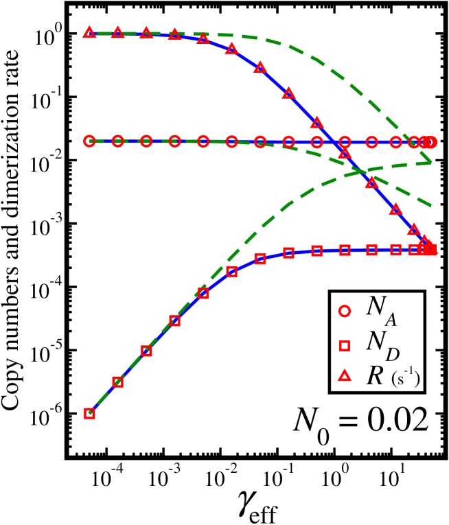
Figure 7: (color online) The average monomer copy number, $\langle N_{A}\rangle^{\rm ss}$ (circles), the average dimer copy number, $\langle N_{D}\rangle^{\rm ss}$ (squares) and the dimerization rate, $\langle R\rangle^{\rm ss}$ (triangles), versus the effective reaction strength parameter, $\gamma_{\rm eff}$, as obtained from the moment equations for the dimerization-dissociation reaction. The parameters used here represent the small system limit, namely $N_{0}=0.02$. The moment equation results are in perfect agreement with those obtained from the master equation (solid lines). However the results of the rate equations (dashed lines) show significant deviations.

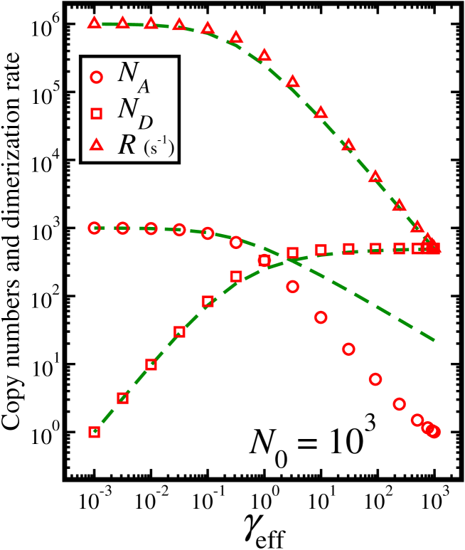
Figure 8: (color online) The average monomer copy number, $\langle N_{A}\rangle^{\rm ss}$ (circles), the average dimer copy number, $\langle N_{D}\rangle^{\rm ss}$ (squares) and the dimerization rate, $\langle R\rangle^{\rm ss}$ (triangles), versus the effective reaction strength parameter, $\gamma_{\rm eff}$, as obtained from the moment equations for the dimerization-dissociation reaction. The parameters used here represent the large system limit, namely $N_{0}=10^{3}$. In this limit the rate equations (dashed lines) are reliable. The moment equation results are in agreement with those obtained from the rate equations for the dimer copy number and its production rate. However, for the monomer copy number, the moment equations deviate in the reaction-dominated limit ($\gamma_{\rm eff}>1$). Slight deviations in the results for $\langle N_{D}\rangle^{\rm ss}$ and $\langle R\rangle^{\rm ss}$ appear around $\gamma_{\rm eff}\simeq 1$, where the crossover from the degradation-dominated regime to the reaction-dominated regime takes place.

In Fig. 7 we present $\langle N_{A}\rangle^{\rm ss}$ (circles), $\langle N_{D}\rangle^{\rm ss}$ (squares) and $\langle R\rangle^{\rm ss}$ (triangles), as obtained from the moment equations for the dimerization-dissociation system versus the effective reaction strength, $\gamma_{\rm eff}$. Here the parameters are $g=0.02$, $d_{1}=1$, $a=2500$ and $d_{2}=1$ (s^-1). The variation of $\gamma_{\rm eff}$ along the horizontal axis was achieved by varying the dissociation rate constant, $u$. For these parameters the system is in the small population limit, namely $N_{0}\ll 1$. The moment equation results are found to be in perfect agreement with the results obtained from the master equations (solid lines). However, the rate equations (dashed lines) show significant deviations for a wide range of parameters. These deviations are largest when the dimerization process is dominant ($\gamma_{\rm eff}>1$) as the effects of stochasticity become important. In Fig. 8 we present $\langle N_{A}\rangle^{\rm ss}$ (circles), $\langle N_{D}\rangle^{\rm ss}$ (squares) and $\langle R\rangle^{\rm ss}$ (triangles), as obtained from the moment equations, versus the effective reaction strength, $\gamma_{\rm eff}$. Here the parameters are $g=1000$, $d_{1}=1$, $a=1$ and $d_{2}=1$ (s^-1). The dissociation rate constant, $u$, was varied. For these parameters the system is in the large population limit, namely $N_{0}\gg 1$. Although the population sizes of the monomer and of the dimer are large, the moment equations are in perfect agreement with the rate equations (dashed lines) in the limit of $\gamma_{\rm eff}\ll 1$. For $\gamma_{\rm eff}\gg 1$ this agreement is maintained for the dimer population size and for its production rate. In this limit the monomer population size is not accounted for by the moment equations. Slight deviations in $\langle N_{D}\rangle$ and $\langle R\rangle$ appear within a narrow range around $\gamma_{\rm eff}\simeq 1$. In this narrow range the effective reaction strength parameter is far away from either of its limiting values. In any case, these deviations are insignificantly small.

In the case of the dimerization-dissociation process the moment equations (49) are a set of three linear coupled differential equations. As opposed to the case of dimerization without dissociation, here the equation for $\langle N_{D}\rangle$ does not only receive input from the other two equations, but also generates an output into those equations. This does not enable one to solve the first and third equations independently to obtain a time dependent solution as shown in the previous Section. Here the time dependent solution will include three characteristic time scales for the relaxation times of both $\langle N_{A}\rangle$, $\langle N_{D}\rangle$ and $\langle R\rangle$. To obtain these time scales we first write Eqs. (49) in matrix form as

$$\dot{\vec{N}}={\bf M}\vec{N}+\vec{b},$$ (51)

where $\vec{N}=(\langle N_{A}\rangle,\langle N_{D}\rangle,\langle R\rangle)$, $\vec{b}=(g,0,0)$ and

$${\bf M}=\left(\begin{array}[]{ccc}-d_{1}&2u&-2\\ 0&-(u+d_{2})&1\\ 2ag&2au&-2(d_{1}+a)\end{array}\right).$$ (55)

The time dependent solution of the moment equations is given by

$$N_{i}=N_{i}^{\rm ss}+\sum_{j=1}^{3}{{\bf C}_{ij}e^{-{t}/{\tau_{j}}}},$$ (56)

where $i,j=1,2,3$. Here, $\vec{N}^{\rm ss}=(\langle N_{A}\rangle^{\rm ss},\langle N_{D}\rangle^{\rm ss},\langle R\rangle^{\rm ss})$, and the matrix elements ${\bf C}_{ij}$ are determined by the initial conditions of the system. The relaxation times $\tau_{j}$ are

$$\tau_{j}=-\frac{1}{\lambda_{j}},$$ (57)

where $\lambda_{j}$, $j=1,2,3$, are the eigenvalues of the matrix ${\bf M}$ [Eq. (55)]. The time dependent solution obtained from the moment equations applies in the limits where $N_{0}\ll 1$, or in the limits where $N_{0}\gg 1$ and $\gamma_{\rm eff}\ll 1$. In the limit where $N_{0}\gg 1$ and $\gamma_{\rm eff}\gg 1$, the time dependent solution should be obtained from the rate equations [Eqs. (44)].

IV Hetero-dimer Production

Consider the case where the reacting monomers are from two different types of molecules, $A$ and $B$. Each of these molecules is generated at a rate $g_{A}$ ($g_{B}$) and degraded at a rate $d_{A}$ ($d_{B}$). The two molecules react to form the dimer $D=AB$ at a rate $a$ (s^-1). The dimer product undergoes degradation at a rate $d_{D}$ (s^-1). For simplicity, here we assume that the process of the dimer dissociation is suppressed. The chemical processes in this system are thus

$$\varnothing\overset{g_{A}}{\longrightarrow}A$$

$$\varnothing\overset{g_{B}}{\longrightarrow}B$$

$$A\overset{d_{A}}{\longrightarrow}\varnothing$$

$$B\overset{d_{B}}{\longrightarrow}\varnothing$$

$$A+B\overset{a}{\longrightarrow}D$$

$$D\overset{d_{D}}{\longrightarrow}\varnothing.$$ (58)

The average copy numbers of the reactive monomers and of the dimer product are described by the following set of rate equations

$$\frac{d\langle N_{A}\rangle}{dt} = g_{A}-d_{A}\langle N_{A}\rangle-\langle R\rangle$$

$$\frac{d\langle N_{B}\rangle}{dt} = g_{B}-d_{B}\langle N_{A}\rangle-\langle R\rangle$$

$$\frac{d\langle N_{D}\rangle}{dt} = -d_{D}\langle N_{D}\rangle+\langle R\rangle,$$ (59)

where $\langle R\rangle$, the dimer production rate, is given by

$$\langle R\rangle=a\langle N_{A}\rangle\langle N_{B}\rangle.$$ (60)

The master equation for this system describes the time evolution of the probabilities $P(N_{A},N_{B},N_{D})$ for a population $N_{A}$ molecules of type $A$, $N_{B}$ molecules of type $B$ and $N_{D}$ dimers $D$ in the system. It takes the form

$$\frac{dP(N_{A},N_{B},N_{D})}{dt} = g_{A}[P(N_{A}-1,N_{B},N_{D})-P(N_{A},N_{B},N_{D})]$$

$$+ g_{B}[P(N_{A},N_{B}-1,N_{D})-P(N_{A},N_{B},N_{D})]$$

$$+ d_{A}[(N_{A}+1)P(N_{A}+1,N_{B},N_{D})-N_{A}P(N_{A},N_{B},N_{D})]$$

$$+ d_{B}[(N_{B}+1)P(N_{A},N_{B}+1,N_{D})-N_{B}P(N_{A},N_{B},N_{D})]$$

$$+ d_{D}[(N_{D}+1)P(N_{A},N_{B},N_{D}+1)-N_{D}P(N_{A},N_{B},N_{D})]$$

$$+ a[(N_{A}+1)(N_{B}+1)P(N_{A}+1,N_{B}+1,N_{D}-1)-N_{A}N_{B}P(N_{A},N_{B},N_{D})]$$

In the stochastic description the production rate of the dimer $D$ is proportional to the number of pairs of $A$ and $B$ molecules in the system, namely

$$\langle R\rangle=a\langle N_{A}N_{B}\rangle.$$ (62)

A more compact stochastic description can be obtained from the moment equations. Here one must include equations for the first moments $\langle N_{A}\rangle$, $\langle N_{B}\rangle$ and $\langle N_{D}\rangle$, and for the production rate, which involves the second moment $\langle N_{A}N_{B}\rangle$. The results for the first moments can be obtained by tracing over the master equation as shown in Sec. II. However, when deriving the equation for $\langle R\rangle$ one obtains

$$\frac{d\langle R\rangle}{dt} = ag_{B}\langle N_{A}\rangle+ag_{A}\langle N_{B}\rangle-(d_{A}+d_{B})\langle R\rangle$$ (63)

$$- a^{2}(\langle{N_{A}}^{2}N_{B}\rangle+\langle N_{A}{N_{B}}^{2}\rangle-\langle N_{A}N_{B}\rangle),$$

which includes third moments for which we have no equations. To obtain the closure condition we follow the procedure presented in Sec. II and impose highly restrictive cutoffs on the master equation. Here the cutoffs are chosen as $N_{A}^{\rm max}=N_{B}^{\rm max}=N_{D}^{\rm max}=1$. These are the minimal cutoffs that enable the dimerization process to take place. Under these cutoffs, the third order moments appearing in Eq. (63) can be expressed by Barzel2007

$$\langle{N_{A}}^{2}N_{B}\rangle=\langle N_{A}{N_{B}}^{2}\rangle=\langle N_{A}N_{B}\rangle.$$ (64)

One then obtains a closed set of moment equations

$$\frac{d\langle N_{A}\rangle}{dt} = g_{A}-d_{A}\langle N_{A}\rangle-\langle R\rangle$$

$$\frac{d\langle N_{B}\rangle}{dt} = g_{B}-d_{B}\langle N_{B}\rangle-\langle R\rangle$$

$$\frac{d\langle N_{D}\rangle}{dt} = -d_{D}\langle N_{D}\rangle+\langle R\rangle$$

$$\frac{d\langle R\rangle}{dt} = ag_{B}\langle N_{A}\rangle+ag_{A}\langle N_{B}\rangle-(d_{A}+d_{B}+a)\langle R\rangle.$$ (65)

As in the case of the homo-molecular dimerization presented above, the validity of the moment equations extends well beyond the cutoff restriction. It can be characterized by four parameters. The first two are $N_{0}^{A}=g_{A}/d_{A}$ and $N_{0}^{B}=g_{B}/d_{B}$, which provide the upper limits on the monomer population sizes $\langle N_{A}\rangle^{\rm ss}$ and $\langle N_{B}\rangle^{\rm ss}$, respectively. The second two parameters are the reaction strength parameters, which in the case of hetero-dimer production are $\gamma_{A}=ag_{A}/(d_{A}d_{B})$ and $\gamma_{B}=ag_{B}/(d_{A}d_{B})$. In the limit where the populations are small, the moment equations provide accurate results for all the moments appearing in Eqs. (65). When the populations are large, the moment equations provide accurate results for the dimerization rate, $\langle R\rangle$, and for the dimer population $\langle N_{D}\rangle$. However, if the reaction strength parameters are also large, the moment equations will not correctly account for the monomer population sizes, $\langle N_{A}\rangle$ and $\langle N_{B}\rangle$.

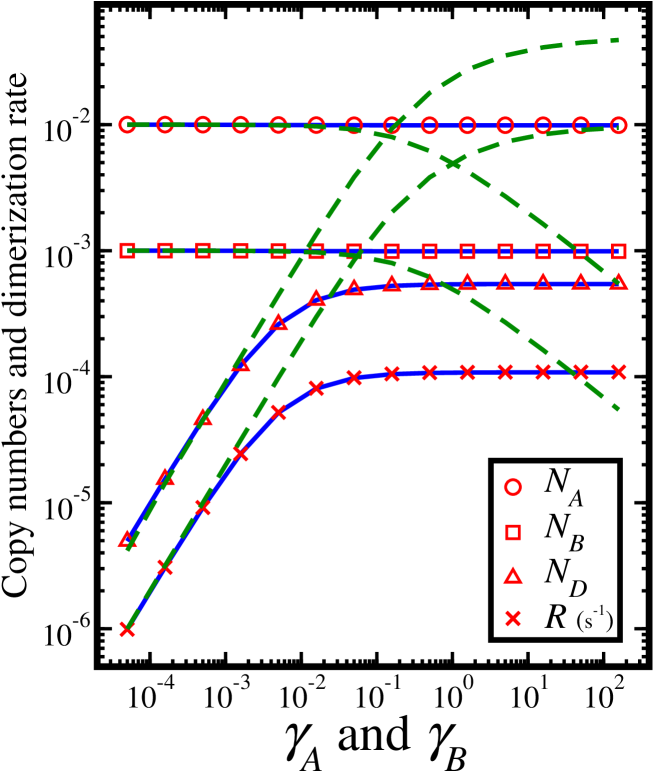
Figure 9: (color online) The average monomer copy numbers, $\langle N_{A}\rangle^{\rm ss}$ (circles) and $\langle N_{B}\rangle^{\rm ss}$ (squares), the average dimer copy number, $\langle N_{D}\rangle^{\rm ss}$ (triangles), and the dimerization rate, $\langle R\rangle^{\rm ss}$ ($\times$), versus the reaction strength parameters, $\gamma_{A}=\gamma_{B}$, as obtained from the moment equations, for the hetero-dimer production system. The parameters used here represent the small system limit. The moment equation results are in perfect agreement with those obtained from the master equation (solid lines). However the results of the rate equations (dashed lines) show significant deviations.

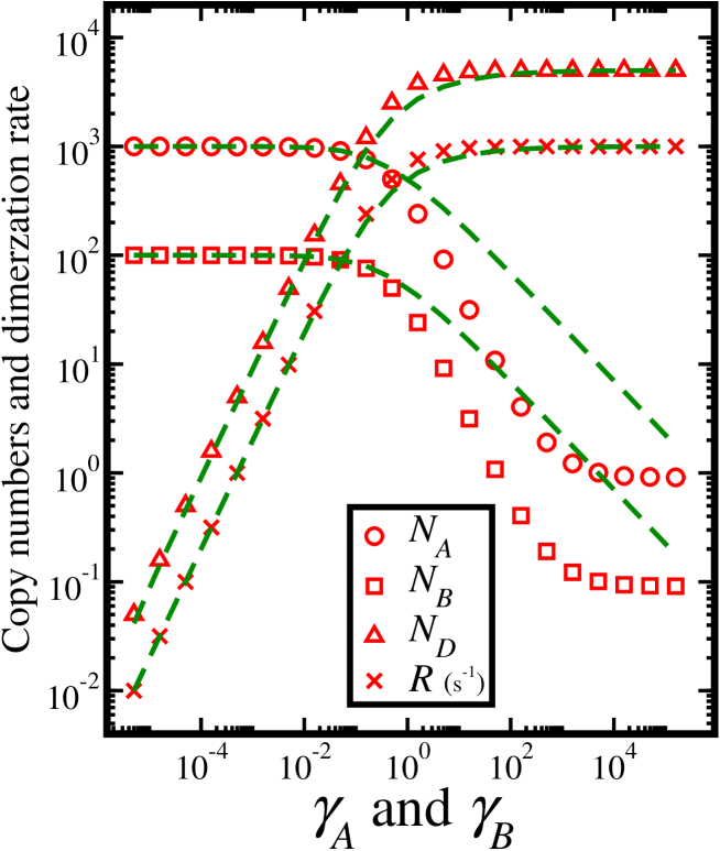
Figure 10: (color online) The average monomer copy numbers, $\langle N_{A}\rangle^{\rm ss}$ (circles) and $\langle N_{B}\rangle^{\rm ss}$ (squares), the average dimer copy number, $\langle N_{D}\rangle^{\rm ss}$ (triangles), and the dimerization rate, $\langle R\rangle^{\rm ss}$ ($\times$), versus the reaction strength parameters, $\gamma_{A}=\gamma_{B}$, as obtained from the moment equations for the hetero-dimer production system. The parameters used here represent the large system limit. In this limit the rate equations (dashed lines) are reliable. The moment equation results are in agreement with the results obtained from the rate equations for the dimer population and its production rate. However, for the monomer copy numbers, the moment equations deviate in the reaction-dominated limit ($\gamma_{A(B)}>1$).

In Fig. 9 we present $\langle N_{A}\rangle^{\rm ss}$ (circles), $\langle N_{B}\rangle^{\rm ss}$ (squares), $\langle N_{D}\rangle^{\rm ss}$ (triangles) and $\langle R\rangle^{\rm ss}$ ($\times$), versus the reaction strength parameters $\gamma_{A}=\gamma_{B}$, as obtained from the moment equations. Here the parameters are $g_{A}=10^{-2}$, $g_{B}=10^{-2}$, $d_{A}=1$, $d_{B}=10$, $d_{D}=0.2$ (s^-1), and the parameter $a$ is varied. These parameters are within the limit of small populations. The results are in perfect agreement with those obtained from the master equation (solid lines). The rate equations (dashed lines) show strong deviations, which are mainly expressed in the reaction-dominated regime. In Fig. 10 we present $\langle N_{A}\rangle^{\rm ss}$ (circles), $\langle N_{B}\rangle^{\rm ss}$ (squares), $\langle N_{D}\rangle^{\rm ss}$ (triangles) and $\langle R\rangle^{\rm ss}$ ($\times$), versus the reaction strength parameters $\gamma_{A}=\gamma_{B}$, as obtained from the moment equations. Here the parameters are $g_{A}=10^{3}$, $g_{B}=10^{3}$, $d_{A}=1$, $d_{B}=10$, $d_{D}=0.2$ (s^-1), and the parameter $a$ is varied. These parameters are within the limit of large populations. Nevertheless the results obtained from the moment equations for $\langle N_{D}\rangle^{\rm ss}$ and for $\langle R\rangle^{\rm ss}$ are in good agreement with those obtained from the rate equations (dashed lines) in both the reaction-dominated limit and in the degradation-dominated limit. For the monomer population sizes, $\langle N_{A}\rangle^{\rm ss}$ and $\langle N_{B}\rangle^{\rm ss}$, the moment equations apply only in the limit where $\gamma_{A}<1$ and $\gamma_{B}<1$.

V Summary and Discussion

We have addressed the problem of dimerization reactions under conditions in which fluctuations are important. We focused on two types of reactions, homo-molecular dimerization ($A+A\rightarrow A_{2}$) and hetero-dimer production ($A+B\rightarrow AB$). Common approaches for the stochastic simulation of such reaction systems include the direct integration of the master equation and Monte Carlo simulations. The master equation involves a large number of coupled equations, for which there is no analytical solution in the time-dependent case. Monte Carlo simulations are often computationally intensive and require averaging over large sets of data. As a result, the relaxation times and the steady state populations for given values of the rate constants can only be obtained by numerical calculations.

Here we have utilized the recently proposed moment equations method, in order to obtain an analytical solution for the relaxation times and for the steady state populations. The moment equations provide an accurate description of dimerization processes in the stochastic limit, at the cost of no more than three or four coupled linear differential equations. Another useful feature of these equations is that in certain cases they also apply in the deterministic limit. Using the moment equations we obtained a complete time dependent solution for the monomer population $\langle N_{A}\rangle$, the dimer population $\langle N_{D}\rangle$ and the dimerization rate $\langle R\rangle$, in the case of homo-molecular dimerization. Expressions for the relaxation times and the steady state populations were found in terms of the rate constants of the different processes. In the case of hetero-dimer production the moment equations include four coupled linear equations. These equations can be easily solved by direct numerical integration. However, a general algebraic expression for this solution is tedious and was not pursued in this paper. Stochastic dimerization processes appear in many natural systems. Below we discuss several examples.

One of the most fundamental chemical reactions taking place in the interstellar medium is hydrogen recombination, namely ${\rm H}+{\rm H}\rightarrow{\rm H}_{2}$ Gould1963 ; Hollenbach1970 ; Hollenbach1971a ; Hollenbach1971b . This reaction occurs on the surfaces of microscopic dust grains in interstellar clouds Spitzer1978 ; Hartquist1995 ; Herbst1995 . The resulting ${\rm H}_{2}$ molecules participate in further reactions in the gas phase, giving rise to more complex molecules Tielens2005 . They also play an important role in cooling processes during gravitational collapse and star formation. In recent years there has been much activity in the computational modeling of interstellar chemistry. While the gas phase chemistry can be simulated by rate equations Pickles1977 ; Hasegawa1992 , the reactions taking place on the dust grain surfaces often require stochastic methods Biham2001 ; Green2001 ; Charnley2001 . This is because under the extreme interstellar conditions of low gas density, the population sizes of the reacting H atoms on the surfaces of these microscopic grains are small and highly fluctuative Tielens1982 ; Charnley1997 ; Caselli1998 ; Shalabiea1998 . The processes taking place on the grains are the accretion of H atoms onto the surface, the desorption of H atoms from the surface, and the diffusion of atoms between adsorption sites on the surface. These processes can be described by the dimerization system discussed in Sec. II. In recent years, experimental work was carried out in an effort to obtain the relevant rate constants and for certain grain compositions these constants were found Pirronello1997a ; Katz1999 ; Hornekaer2003 ; Perets2005 ; Perets2007 . The solution of the moment equations, as appears in Sec. II, provides the production rate of molecular hydrogen on interstellar dust grains, in the limit of small grains and low fluxes, where fluctuations are important.

In the biological context, regulation processes in cells can be described by networks of interacting genes Alon2006 ; Palsson2006 . The interactions between genes include transcriptional regulation processes as well as protein-protein interactions Yeger-Lotem2004 . Due to the small size of the cells, some of these proteins my appear in low copy numbers, with large fluctuations McAdams1997 ; Paulsson2000 ; Paulsson2004 ; Friedman2006 . Deterministic methods are thus not suitable for the modeling of these systems. Dimerization of proteins is a common process in living cells. In particular, many of the transcriptional regulator proteins bind to their specific promoter sites on the DNA in the form of dimers. It turns out that such dimerization, taking place before binding to the DNA, provides an effective mechanism for the reduction of fluctuations in the monomer copy numbers Bundschuh2003 .

In a broader perspective, complex reaction networks appear in a variety of physical contexts. The building blocks of these networks are intra-species interactions and inter-species interactions. Thus, the analysis presented in this paper of homo-molecular and hetero-molecular dimerization processes, lays the foundations for the analysis of more complex networks. Complex stochastic networks are difficult to simulate using standard methods, because they require exceedingly long simulation times. The moment equations, applied here to dimerization systems, provide a highly efficient method for the simulation of complex chemical networks.

This work was supported by the US-Israel Binational Science Foundation and by the France-Israel High Council for Science and Technology Research.

Table 1: The validity ($\surd$) or invalidity ($\times$) of the moment equations for the evaluation of $\langle N_{A}\rangle$, $\langle N_{D}\rangle$ and $\langle R\rangle$ in the different limits of the dimerization system. The results for $\langle N_{D}\rangle$ and $\langle R\rangle$ are valid in all limits. The results for $\langle N_{A}\rangle$ are invalid in the limit of large systems and reaction-dominated kinetics.

	$N_{0}\ll 1$		$N_{0}\gg 1$
	$\gamma\ll 1$	$\gamma\gg 1$	$\gamma\ll 1$	$\gamma\gg 1$
$\langle N_{A}\rangle$	$\surd$	$\surd$	$\surd$	$\times$
$\langle N_{D}\rangle$	$\surd$	$\surd$	$\surd$	$\surd$
$\langle R\rangle$	$\surd$	$\surd$	$\surd$	$\surd$

Table 2: The relaxation times for $\langle N_{A}\rangle$ and $\langle N_{D}\rangle$ in the different limits of the dimerization system. For the monomer population the relaxation time is determined by the degradation rate, $d_{1}$ in three of the four limits. In the reaction-dominated, large system limit the relaxation time is determined by $\sqrt{8ag}$. In case that the degradation rate of the dimer, $d_{2}$, is large, its relaxation follows that of the monomer population. Otherwise, it is determined by $d_{2}$.

	$N_{0}\ll 1$		$N_{0}\gg 1$
	$\gamma\ll 1$	$\gamma\gg 1$	$\gamma\ll 1$	$\gamma\gg 1$
$\tau_{A}$	$\frac{1}{d_{1}}$			$\frac{1}{\sqrt{8ag}}$
$\tau_{D}$	$\max\left(\frac{1}{d_{1}},\frac{1}{d_{2}}\right)$			$\max\left(\frac{1}{\sqrt{8ag}},\frac{1}{d_{2}}\right)$

Figure 1: Dimerization systems can be classified into four different regimes, characterized by the system size parameter, $N_{0}=g/d_{1}$, and by the reaction strength parameter $\gamma=ag/d_{1}^{2}$. In the large system limit, where $N_{0}\gg 1$ (quadrants II and IV), the monomer copy number is typically large, and the fluctuation level of the system is low. In the small system limit, where $N_{0}\ll 1$ (quadrants I and III), the monomer copy number is low, and the system becomes dominated by fluctuations. The reaction strength parameter characterizes the dominant dynamical process in the system. In the limit where $\gamma\gg 1$ (quadrants I and II) the process of dimerization is dominant, and the degradation is suppressed. In the limit where $\gamma\ll 1$ (quadrants III and IV) the degradation process is dominant, and only a small fraction of the monomers undergo dimerization.

References

- (1) N.G. van Kampen, Stochastic Processes in Physics and Chemistry (North-Holland, Amsterdam, 1981).
- (2) C.W. Gardiner, Handbook of Stochastic Methods (Springer, Berlin, 2004).
- (3) O. Biham, I. Furman, V. Pirronello and G. Vidali, Astrophys. J. 553, 595 (2001).
- (4) N.J.B. Green, T. Toniazzo, M.J. Pilling, D.P. Ruffle, N. Bell and T.W. Hartquist, Astron. Astrophys. 375, 1111 (2001).
- (5) D.T. Gillespie, J. Comput. Physics 22, 403 (1976).
- (6) D.T. Gillespie, J. Phys. Chem. 81, 2340 (1977).
- (7) A.G.G.M. Tielens and W. Hagen, Astron. Astrophys. 114, 245 (1982).
- (8) M.E.J. Newman and G.T. Barkema, Monte Carlo methods in statistical physics (Clarendon Press, Oxford, 1999).
- (9) S.B. Charnley, Astrophys. J. 562, L99 (2001).
- (10) O. Biham and A. Lipshtat, Phys. Rev. E 66, 056103 (2002).
- (11) T. Stantcheva, V.I. Shematovich and E. Herbst, Astron. Astrophys. 391, 1069 (2002).
- (12) T. Stantcheva and E. Herbst, Mon. Not. R. Astron. Soc. 340, 983 (2003).
- (13) A. Lipshtat, O. Biham, Astron. Astrophys. 400, 585 (2003).
- (14) B. Barzel and O. Biham, Astrophys. J. 658, L37 (2007).
- (15) B. Barzel and O. Biham, J. Chem. Phys. 127, 144703 (2007).
- (16) A. Lederhendler and O. Biham, Phys. Rev. E 78, 041105 (2008).
- (17) F.S. Acton, Numerical Methods that Work (The Mathematical Association of America, New York, 1970).
- (18) W. H. Press, S. A. Teukpolsky, W. T. Vetterling & B. P. Flannery, Numerical Recipes: The Art of Scientific Computing (Cambridge University Press, Cambridge, 1992).
- (19) D.A. McQuarrie, J. Appl. Prob. 4, 413 (1967).
- (20) C.A. Gómez-Uribe and G.C. Verghese, J. Chem. Phys. 126, 024109 (2007).
- (21) R.J. Gould and E.E. Salpeter, Astrophys. J. 138, 393 (1963).
- (22) D. Hollenbach and E.E. Salpeter, J. Chem. Phys. 53, 79 (1970).
- (23) D. Hollenbach and E.E. Salpeter, Astrophys. J. 163, 155 (1971).
- (24) D. Hollenbach, M.W. Werner and E.E. Salpeter, Astrophys. J. 163, 165 (1971).
- (25) L. Spitzer, Physical Processes in the Interstellar Medium (Wiley, New York, 1978).
- (26) T.W. Hartquist and D.A. Williams, The chemically controlled cosmos (Cambridge University Press, Cambridge, UK, 1995).
- (27) E. Herbst, Annu. Rev. Phys. Chem. 46, 27 (1995).
- (28) A.G.G.M. Tielens, The Physics and Chemistry of the Interstellar Medium (Cambridge University Press, Cambridge, 2005).
- (29) J.B. Pickles and D.A. Williams, ApSS 52, 433 (1977).
- (30) T.I. Hasegawa and E. Herbst and C.M. Leung, ApJ Supplement 82, 167 (1992).
- (31) S.B. Charnley, A.G.G.M. Tielens and S.D. Rodgers, Astrophys. J. 482, L203 (1997).
- (32) P. Caselli, T.I. Hasegawa and E. Herbst, Astrophys. J. 495, 309 (1998).
- (33) O.M. Shalabiea, P. Caselli and E. Herbst, Astrophys. J. 502, 652 (1998).
- (34) N. Katz, I. Furman, O. Biham, V. Pirronello and G. Vidali, Astrophys. J. 522, 305 (1999).
- (35) H.B. Perets, O. Biham, V. Pirronello, J.E. Roser, S. Swords, G. Manico and G. Vidali, Astrophys. J. 627, 850 (2005).
- (36) H.B. Perets, A. Lederhendler, O. Biham, G. Vidali, L. Li, S. Swords, E. Congiu, J. Roser, G. Manicó, J.R. Brucato and V. Pirronello, Astrophys. J. 661, L163 (2007).
- (37) V. Pirronello, C. Liu, L. Shen and G. Vidali, Astrophys. J. 475, L69 (1997).
- (38) L. Hornekaer, A. Baurichter, V.V. Petrunin, D. Field and A.C. Luntz, Science 302, 1943 (2003).
- (39) U. Alon, An introduction to systems biology: design principles of biol ogical circuits (Chapman & Hall/CRC, London, 2006).
- (40) B.Ø. Palsson, Systems biology: properties of reconstructed networks (Cambridge University Press, Cambridge, 2006).
- (41) E. Yeger-Lotem, S. Sattath, N. Kashtan, S. Itzkovitz,R. Milo, R.Y. Pinter, U. Alon and H. Margalit, Proc. Natl. Acad. Sci. US 101, 5934 (2004).
- (42) H.H. McAdams and A. Arkin, 94, 814 (1997).
- (43) J. Paulsson and M. Ehrenberg, Phys. Rev. Lett. 84, 5447 (2000).
- (44) J. Paulsson, Nature 427, 415 (2004).
- (45) N. Friedman, L. Cai and X.S. Xie, Phys. Rev. Lett. 97, 168302 (2006).
- (46) R. Bundschuh, F. Hayot and C. Jayaprakash, J. Theor. Biol. 220, 261 (2003).