Abstract

We consider a supersymmetric (SUSY) scenario including right-handed neutrinos, one of whose scalar superpartners is the lightest SUSY particle (LSP). The distinguishing feature in the collider signal of SUSY in such a case is not missing energy but a pair of charged tracks corresponding to the next-to-lightest SUSY particle, when it is, as in the case considered, a stau. Following up on our recent work on neutralino reconstruction in such cases, we explore the possibility of reconstructing charginos, too, through a study of transverse mass distributions in specified final states. The various steps of isolating the transverse momenta of neutrinos relevant for this are outlined, and regions of the parameter space where our procedure works are identified.

1 Introduction

If supersymmetry (SUSY) [1, 2], broken at the TeV scale, has to validate itself as the next step in physics beyond the standard model (SM), then it is likely to be discovered at the Large Hadron Collider (LHC), with the superpartners of the SM particles being identified. It is therefore of great importance to make a thorough inventory of collider signals answering to various SUSY scenarios. These can serve not only to unveil the general character of the scenario but also to yield a wealth of information as possible about the specific properties of the new particles.

One attractive feature of supersymmetric theories, in the $R$-parity (defined as $R=(-)^{3B+L+2S}$) conserving form, is that the superparticles are always produced in pairs and each interaction vertex must involve an even number of superparticles (having R = -1). Hence the lightest SUSY particle (LSP) is stable and all SUSY cascades at the collider experiments should end up with the pair production of the LSP. As a bonus, it provides a viable candidate for dark matter (DM) if the LSP is electrically neutral and only weakly interacting. Since the LSP, due to such a character, escapes the detector without being detected, a prototype signature of $R$-conserving SUSY is energetic jets and/or leptons associated with large missing transverse energy ($/\!\!\!E_{T}$).

However, there can be several SUSY models [3] which include a quasi-stable next-to-lightest supersymmetric particle (NLSP). This can happen in cases where the NLSP is nearly degenerate in mass with the LSP, or if its coupling to the LSP is too small. Hence the decay width of the NLSP into the LSP is highly suppressed. Consequently the NLSP becomes stable on the detector scale, its lifetime being long enough to escape the detector without decaying inside it. Thus the NLSP behaves like a stable particle within the detector. The resulting collider signals change drastically, especially if the NLSP is a charged particle. The quintessential SUSY signals then is not $/\!\!\!E_{T}$ but two hard charged tracks of massive stable particles which appear as far as up to the muon chamber. This opens up a whole set of new possibilities for collider studies, including reconstruction of the sparticle masses, something that is relatively more difficult in the presence of $/\!\!\!E_{T}$.

The scenario we have considered here, as an illustration of such a quasi-stable NLSP, is the minimal supersymmetric standard model (MSSM) augmented with a right-chiral Dirac-type neutrino superfields for each generation. This is consistent with the existing evidence [4] of neutrino masses and mixing, although no explanation for the smallness of neutrino masses is offered. It is possible in such a case to have an LSP is dominated by this right-chiral sneutrino state ($\tilde{\nu}_{R}$) together with a charged particle as the NLSP. We specifically consider a situation with a stau ($\tilde{\tau}$) NLSP . Such a scenario can easily be motivated [7] by assuming that the MSSM is embedded in a high scale framework of SUSY breaking. As we shall see, this can happen in minimal supergravity (mSUGRA) [8] where the masses evolve from “universal” scalar ($m_{0}$) and gaugino ($M_{1/2}$) mass parameters at a high scale. The only extension here is the right-chiral neutrino superfield (in fact, three of them) whose scalar component derives its soft mass from the same $m_{0}$. The existence of such a quasistable charged slepton can be well in agreement with the observed abundance of light elements as predicted by the big-bang nucleosynthesis (BBN) [9], provided, its mass is below a TeV. Since the right-chiral sneutrino has no gauge couplling but only interactions proportional to the neutrino Yukawa coupling, the strength of which is too feeble to be seen in dark matter search experiments, such an LSP is consistent with all direct searches carried out so far. Moreover, it has been shown that such a spectrum is consistent with all low energy constraints [10], and the contribution to the relic density of the universe can be compatible with the limits set by the Wilkinson Microwave Anisotropy Probe (WMAP) [11] with appropriate values of the relevant parameters [12].

In this work, we have concentrated on the mass reconstruction of the lightest chargino in a $\tilde{\tau}$-NLSP, $\tilde{\nu}_{1}$-LSP scenario. This is a follow-up of our earlier work [13] on neutrlino reconstruction under similar circumstances. We have shown that it is possible to determine the mass of the lightest chargino, produced in the cascade decay of squarks or gluinos, from the sharp drop noticed in the transverse mass [14] distribution of the chargino decay products. More precisely, we show a way of disentangling the transverse mass of the system consisting of a $\tilde{\tau}$-track and the associated neutrino from chargino decay. We suggest a method for extracting the transverse momentum ($p_{T}$) of the neutrino. Though a sizable statistics is required for this purpose, and one may have to wait for considerable accumulated luminosity after the discovery of the LHC, still this is a rather spectacular prospect. We have successfully applied the criteria, developed in our earlier work, for separating the signal from standard model backgrounds. Ways of suppressing SUSY processes that are likely to contaminate the transverse mass distributions are also suggested.

It should be mentioned that neither the signal we have studied nor the prescribed reconstruction technique is limited just to scenarios with right-sneutrino LSP. It can be applied successfully to all cases [15, 16, 17] where the NLSP is a charged scalar with quasi-stable character, provided that it decays outside the detector, leaving behind a charged track in the muon chamber.

The paper is organized as follows: in Sec. 2, we motivate the scenario under investigation and present a brief review of the mass reconstruction for neutralinos as done in the earlier paper and used in this work. There we also summarise our choice of benchmark points. The signal under study and the reconstruction strategy for determining the chargino mass as well as the possible sources of background, both from the SM and within the model itself, and their possible discrimination, are discussed in Sec. 3. We summarise and conclude in Sec. 4.

2 The overall scenario, mass reconstruction and representative benchmark points

2.1 Scenarios with $\tilde{\nu}_{R}$ LSP and $\tilde{\tau}$ NLSP

As has been already stated, the most simple-minded extension of the MSSM [18], accommodating neutrino masses, is the addition of one right-handed neutrino superfield per family. In this situation the neutrinos have Dirac masses induced by very small Yukawa couplings. The superpotential of such an extended MSSM becomes (suppressing family indices),

$$W_{MSSM}=y_{l}\hat{L}\hat{H_{d}}\hat{E^{c}}+y_{d}\hat{Q}\hat{H_{d}}\hat{D^{c}}+y_{u}\hat{Q}\hat{H_{u}}\hat{U^{c}}+\mu\hat{H_{d}}\hat{H_{u}}+y_{\nu}\hat{H}_{u}\hat{L}\hat{\nu}^{c}_{R}$$ (1)

where $\hat{H_{d}}$ and $\hat{H_{u}}$, respectively, are the Higgs superfields that give masses to the $T_{3}=-1/2$ and $T_{3}=+1/2$ fermions, and $y^{\prime}s$ are the strengths of Yukawa interaction. $\hat{L}$ and $\hat{Q}$ are the left-handed lepton and quark superfields respectively, whereas $\hat{E^{c}}$, $\hat{D^{c}}$ and $\hat{U^{c}}$, in that order, are the right handed gauge singlet charged lepton, down-type and up-type quark superfields. $\mu$ is the Higgsino mass parameter.

It is a common practice to attempt reduction of free parameters in the theory, by assuming a high-scale framework of SUSY breaking. The most commonly adopted scheme is based on N = 1 minimal supergravity (mSUGRA). There SUSY breaking in the hidden sector at high scale is manifested in universal soft masses for scalars ($m_{0}$) and gauginos ($M_{1/2}$), together with the trilinear ($A$) and bilinear ($B$) SUSY breaking parameters in the scalar sector. The bilinear parameter is determined by the electroweak symmetry breaking (EWSB) conditions. All the scalar and gaugino masses at low energy obtained by renormalization group evolution (RGE) of the universal mass parameters $m_{0}$ and $M_{1/2}$ from high-scale values [19]. Thus one generates all the squark, slepton, and gaugino masses as well as all the mass parameters in the Higgs sector. The Higgsino mass parameter $\mu$ (up to a sign), too is determined from EWSB conditions. All one has to do in this scheme is to specify the high scale ($m_{0},M_{1/2},A_{0}$, together with $sign(\mu)~{}{\rm and}~{}\tan\beta~{}=~{}\langle H_{u}\rangle/\langle H_{d}\rangle$) where, $\tan\beta$ is the ratio of the vacuum expectation values of the two Higgs doublets that give masses to the up-and down-type quarks respectively.

The neutrino masses are typically given by,

$$m_{\nu}=y_{\nu}\left<H_{u}^{0}\right>=y_{\nu}v~{}\sin\beta$$ (2)

The small Dirac masses of the neutrinos imply that the neutrino Yukawa couplings ($y_{\nu}$) are quite small ($\mathrel{\mathchoice{\lower 1.72218pt\vbox{\halign{$\m@th\displaystyle\hfil#\hfil$\cr<\crcr\sim\crcr}}}{\lower 1.72218pt\vbox{\halign{$\m@th\textstyle\hfil#\hfil$\cr<\crcr\sim\crcr}}}{\lower 1.72218pt\vbox{\halign{$\m@th\scriptstyle\hfil#\hfil$\cr<\crcr\sim\crcr}}}{\lower 1.72218pt\vbox{\halign{$\m@th\scriptscriptstyle\hfil#\hfil$\cr<\crcr\sim\crcr}}}}10^{-13}$).

With the inclusion of the right-chiral neutrino superfields as a minimal extension, it makes sense to assume that the masses of their scalar components, too, originate in the same parameter $m_{0}$. The evolution of all other parameters practically remain the same in this scenario as in the MSSM, while the right-chiral sneutrino mass parameter evolves at the one-loop level [20] as

$$\frac{dM^{2}_{\tilde{\nu}_{R}}}{dt}=\frac{2}{16\pi^{2}}y^{2}_{\nu}~{}A^{2}_{\nu}~{}~{}.$$ (3)

where $A_{\nu}$ is obtained by the running of the trilinear soft SUSY breaking term $A$ and is responsible for left-right mixing in the sneutrino mass matrix.

It follows from above that the value of $M_{\tilde{\nu}_{R}}$ remains practically frozen at $m_{0}$, thanks to the extremely small Yukawa couplings, whereas the other sfermion masses are enhanced at the electroweak scale. Thus, for a wide range of values of the gaugino masses, one naturally ends up with a sneutrino LSP ($\tilde{\nu}_{1}$), dominated by the right-chiral state. This is because the mixing angle is controlled by the neutrino Yukawa couplings:

$$\tilde{\nu}_{1}=-\tilde{\nu}_{L}\sin\theta+\tilde{\nu}_{R}\cos\theta$$ (4)

where the mixing angle $\theta$ is given by,

$$\tan 2\theta=\frac{2y_{\nu}v\sin\beta|\cot\beta\mu-A_{\nu}|}{m^{2}_{\tilde{\nu}_{L}}-m^{2}_{\tilde{\nu}_{R}}}$$ (5)

Of the three charged sleptons, the amount of left-right mixing is always the largest in the third, and hence the lighter stau ($\tilde{\tau}_{1}$) often turns out to be the NLSP in such a scenario. There are regions in the parameter space the three lighter sneutrino states corresponding to the three flavours act virtually as co-LSP’s. It is, however, sufficient for illustrating our points to consider the lighter sneutrino mass eigenstate of the third family, as long as the state ($\tilde{\tau}_{1}$) is the lightest among the charged sleptons. Thus the addition of a right-handed sneutrino superfield, for each family, which is perhaps the most minimal input to explain neutrino masses and mixing, can eminently turn a mSUGRA theory into one with a stau NLSP and a sneutrino LSP. It is should be emphasized that the physical LSP state can have (a) Yukawa couplings proportional to the neutrino mass, and (b) gauge coupling with the small left-chiral admixture in it, driven by left-right mixing which is again proportional to $y_{\nu}$. Thus the decay of any particle (particularly the NLSP) into the LSP will always be a very slow process, not taking place within the detector. Under such circumstances, the quintessential SUSY signal is not $/\!\!\!E_{T}$ anymore but a pair of charged tracks left by the quasi-stable NLSP.

2.2 Neutralino reconstructed

In an earlier study [13], we suggested a reconstruction technique for at least one of the two lightest neutralinos, in the $\tilde{\nu}_{R}$ LSP and $\tilde{\tau}$ NLSP scenario. The signal studied there was: $2\tau_{j}+2\tilde{\tau}(charged-track)+E_{T}/~{}~{}+X$. Here $\tau_{j}$ denotes a jet out of one-prong decays of the tau, and all accompanying hard jets arising from cascades are included in X. The kinematic cuts imposed by us, such as $p^{track}_{T}>$100 GeV and $\sum\vec{|}p_{T}|>$1 TeV, ($p_{T}$ = transverse momentum, and $\sum\vec{|}p_{T}|$ is the scalar sum of all visible tarnsverse momenta) reduced the backgrounds considerably.

Since the signal we investigated involves two taus in the final state, and hadronic decays of tau was considered, tau-jet identification and tau reconstruction were two important components of the procedure. For this a method suggested in [21] was used, which involved solving the following equation event-by-event:

$$\vec{/}\!\!\!p_{T}=({1\over x_{\tau_{h1}}}-1)\;\vec{p}_{h1}+({1\over x_{\tau_{h2}}}-1)\;\vec{p}_{h2}\;$$ (6)

where $x_{\tau_{hi}}$ (i = 1,2) is the fraction of the tau energy carried by each product jet collinear with the parent tau, when it is boosted. $\vec{/}\!\!\!p_{T}$ is the vector sum of the transverse components of the 3-momenta of the two product neutrinos produced in hadronic decay of each tau. Clearly this method is applicable when there is no other invisible particle in the final state. This was ensured in the best possible manner by vetoing any isolated lepton in the final state, thus getting rid of additional neutrinos from W-decays.

The reconstruction of $\vec{/}\!\!\!p_{T}$ is undoubtedly very crucial here. $\vec{/}\!\!\!p_{T}$ is reconstructed as the negative of the total visible $\vec{p_{T}}$ which receives the contributions from isolated leptons/ sleptons, jets and unclustered components. The last among these includes all particles (electron/photon/ muon/stau) with $0.5<E_{T}<10$GeV and $|\eta|<5$ (for muon or muon-like tracks, $|\eta|<2.5$), or hadrons with $0.5<E_{T}<20$GeV and $|\eta|<5$, which do not contribute to a jet and constitute ‘hits’ in the detector [22]. In order to simulate the finite resolution of detectors, the energies/transverse momenta of all particles were smeared following prescriptions detailed in [13].

Once the tau 4-momenta are obtained, they are combined with the staus to find the stau-tau invariant mass distribution. This requires the knowledge of stau mass as well as the choice of the correct pair. The correct pairs are obtained by using a seed mass for $\tilde{\tau}$ which was taken to be 100 GeV, satisfying the criterion $|M^{pair1}_{\tilde{\tau}\tau}-M^{pair2}_{\tilde{\tau}\tau}|<50~{}GeV$. The actual stau mass is then extracted by demanding that the invariant masses of the two $\tilde{\tau}\tau$ pairs were equal, which yields an equation involving one unknown quantity, namely, $m_{\tilde{\tau}}$:

$$\sqrt{m^{2}_{\tilde{\tau}}+|\vec{p_{\tilde{\tau}_{1}}}|^{2}}.E_{\tau_{1}}-\sqrt{m^{2}_{\tilde{\tau}}+|\vec{p_{\tilde{\tau}_{2}}}|^{2}}.E_{\tau_{2}}=\vec{p_{\tilde{\tau}_{1}}}.\vec{p_{\tau_{1}}}-\vec{p_{\tilde{\tau}_{2}}}.\vec{p_{\tau_{2}}}$$ (7)

Having thus extracted $m_{\tilde{\tau}}$ on an event-by-event basis in the event generator, it was demonstrated that the distribution of this mass value has a peak at the actual $m_{\tilde{\tau}}$. We have used this peak value in reconstructing the neutralino from the invariant mass distribution of the $\tilde{\tau}\tau$ pair. In some regions of the parameter space, it is possible to thus reconstruct only $\chi^{0}_{1}$, as the production rate of $\chi^{0}_{2}$ in cascade decay of $\tilde{q}$ (or $\tilde{g}$) as well as the decay branching ratio of $\chi^{0}_{2}\rightarrow\tilde{\tau}\tau$ is small. In some other regions, we have been able to reconstruct both of them. There are still other regions only the $\chi^{0}_{2}$ peak shows up. This is because of the small mass splitting between $\chi^{0}_{1}$ and $\tilde{\tau}$, which softens the tau (jet) arising from its decay, preventing it from passing the requisite hardness cut.

2.3 The choice of benchmark points

The choice of benchmark points for this study is the same as in the case of neutralino reconstruction [13]. The mSUGRA parameter space is utilised for this purpose. A $\tilde{\tau}$ NLSP and a $\tilde{\nu}_{1}$ LSP occur in those regions in which one would have had a $\tilde{\tau}$ LSP in the absence of right-chiral neutrino superfields. We focus on both the regions where (a) $m_{{\tilde{\tau}}_{1}}>m_{{\tilde{\nu}}_{1}}+m_{W}$, and (b) the above inequality is not satisfied. In the first case, the dominant decay mode is the two-body decay of the NLSP, ${\tilde{\tau}}_{1}\to\tilde{\nu}_{1}W$, and, in the second, the decay takes place via a virtual $W$. Decay into a charged Higgs is a subdominant channel for the lighter stau. The decay takes place outside the detector in all cases. At different benchmark points, however, the mass splittings between the $\tilde{\tau}_{1}$ and neutralinos/charginos are different. This in turn affects the kinematic characteristics of the final states under consideration.

We have used the spectrum generator ISAJET 7.78 [23] for our study. In Table-1 we list the six benchmark points used, both in terms of high-scale parameters and low-energy spectra. The justification of their choice and their representative character have been explained in reference [13].

	BP-1	BP-2	BP-3	BP-4	BP-5	BP-6
mSUGRA	$m_{0}=100$	$m_{0}=100$	$m_{0}=100$	$m_{0}=100$	$m_{0}=100$	$m_{0}=100$
input	$m_{1/2}=600$	$m_{1/2}=500$	$m_{1/2}=400$	$m_{1/2}=350$	$m_{1/2}=325$	$m_{1/2}=325$
	$\tan\beta=30$	$\tan\beta=30$	$\tan\beta=30$	$\tan\beta=30$	$\tan\beta=30$	$\tan\beta=25$
$m_{\tilde{e_{L}}},m_{\tilde{\mu}_{L}}$	418	355	292	262	247	247
$m_{\tilde{e_{R}}},m_{\tilde{\mu}_{R}}$	246	214	183	169	162	162
$m_{\tilde{\nu}_{eL}},m_{\tilde{\nu}_{\mu L}}$	408	343	279	247	232	232
$m_{\tilde{\nu}_{\tau L}}$	395	333	270	239	224	226
$m_{\tilde{\nu}_{iR}}$	100	100	100	100	100	100
$m_{\tilde{\tau}_{1}}$	189	158	127	112	106	124
$m_{\tilde{\tau}_{2}}$	419	359	301	273	259	255
$m_{\chi^{0}_{1}}$	248	204	161	140	129	129
$m_{\chi^{0}_{2}}$	469	386	303	261	241	240
$m_{\chi^{\pm}_{1}}$	470	387	303	262	241	241
$m_{\tilde{g}}$	1362	1151	937	829	774	774
$m_{\tilde{t}_{1}}$	969	816	772	582	634	543
$m_{\tilde{t}_{2}}$	1179	1008	818	750	683	709
$m_{h^{0}}$	115	114	112	111	111	111

Table 1: Proposed benchmark points (BP) for the study of the stau-NLSP scenario in SUGRA with right-sneutrino LSP. The values of $m_{0}$ and $M_{1/2}$ are given in GeV. We have also set $A_{0}=100~{}GeV$ and $sgn(\mu)=+$ for benchmark points under study.

It may be noted that the region of the mSUGRA parameter space where we have worked is consistent with all the experimental bounds [24], including both collider and low-energy constraints (such as the LEP and Tevatron constraints on the masses of Higgs, gluinos, charginos etc., as also those from $b\rightarrow s\gamma$, correction to the $\rho$-parameter, ($g_{\mu}-2$) and so on). In the next section we describe the procedure for the reconstruction of $\chi^{\pm}_{1}$, for these benchmark points.

3 Reconstruction of the lighter chargino

The final state of use for the reconstruction of the lighter chargino is

• $\tau_{j}+2\tilde{\tau}{\rm(opposite-sign~{}charged~{}tracks)}+E_{T}/~{}~{}+X$

where, $\tau_{j}$ represents a jet which has been identified as a tau jet, the missing transverse energy is denoted by $E_{T}/~{}~{}$ and all other jets coming from cascade decays are included in X .

Simulation for the LHC has been done for the signal as well as backgrounds using PYTHIA (v6.4.16) [25]. The $pp$ events has been studied with a centre-of-mass energy ($E_{c.m.}$)=14 TeV at an integrated luminosity of 300 $fb^{-1}$. The numerical values of the electromagnetic and the strong coupling constant have been set at $\alpha^{-1}_{em}(M_{Z})=127.9$ and $\alpha_{s}(M_{Z})=0.118$ respectively [10]. The hard scattering process has been folded with CTEQ5L parton distribution function [26]. We have set the factorization and renormalization scales at the average mass of the particles produced in the parton level hard scattering process. In order to make our estimate conservative, the signal rates have not been multiplied by any K-factor [27]. The effects of initial and final state radiation as well as the finite detector resolution of the energies/momenta of the final state particles have been taken into account.

3.1 Chargino reconstruction from transverse mass distribution

Now we are all set to describe the main principle adopted by us for chargino ($\chi^{\pm}_{1}$) reconstruction. For this purpose, we have looked for the processes in which $\chi^{\pm}_{1}-\chi^{0}_{1}/\chi^{0}_{2}$ is being produced in association with hard jets in cascade decays of squarks and gluinos. The $\chi^{\pm}_{1}$ subsequently decays into a $\tilde{\tau}$-$\nu_{\tau}$ pair, while the $\chi^{0}_{1}$ (or $\chi^{0}_{2}$) decays into a $\tilde{\tau}$-$\tau$ pair. Since the decay of $\chi^{\pm}_{1}$ involves an invisible particle ($\nu_{\tau}$), for which it is not possible to know all the four components of momenta, a transverse mass distribution, rather than invariant mass distribution, of $\tilde{\tau}$-$\nu_{\tau}$ pair will give us mass information of $\chi^{\pm}_{1}$. In spite of the recent progress in measuring the masses of particles in semi-invisible decay mode (for example the $m_{T_{2}}$ variable introduced by [28] and its further implications [29]), we have focused on transverse mass variable ($m_{T}$) because of the fact that the only invisible particle present in the final state is the neutrino, which is massless.

The procedure, however, still remains problematic, because the $\tau$ on the other side (arising from neutralino decay) also produces a neutrino in the final state, which contributes to $E_{T}/~{}~{}$. In order to correctly reconstruct the transverse mass of the $\tilde{\tau}-\nu_{\tau}$ pair from chargino decay, the contribution to $E_{T}/~{}~{}$ from the aforementioned neutrino must be subtracted.

Keeping this in mind, we have prescribed a method for reconstruction of the transverse component of the neutrino 4-momenta ($\vec{P}^{T}_{\nu_{1}}$) produced from the decay of $\chi^{\pm}_{1}$, in association with $\tilde{\tau}$. To describe it in short:

We label the transverse momentum of the neutrino coming from chargino decay by $\vec{P}^{T}_{\nu_{1}}$. Attention is focused on cases where the tau, produced from a neutralino, decays hadronically and the $\tau$-jet, out of a one-prong decay of tau, is identified following the prescription of [21]. We have assumed a true tau-jet identification efficiency to be 50$\%$, while a non-tau jet rejection factor of 100 has been used [30, 31, 32] (The results for higher identification efficiency are also shown in Sec. 4.). We have also assumed that there is no invisible particle other than the two neutrinos mentioned above. We have attempted to ensure this by vetoing any event with isolated charged leptons. This only leaves out neutrinos from $Z$-decay and $W$-decays into a $\tau\nu_{\tau}$ pair. The contamination of our signal from these are found to be rather modest.

The transverse momenta of the neutrino ($\vec{P}^{T}_{\nu_{2}}$), out of a tau decay, is first reconstructed in the collinear approximation, where the product neutrino and the jet are both assumed to move collinearly with the parent tau. In this approximation, one can write

$$P_{\tau_{j}}=xP_{\tau}$$ (8)

Following the decay $\chi^{0}_{1}$ (or, $\chi^{0}_{2}$)$\rightarrow\tilde{\tau}^{\pm}\tau^{\mp}$ we have then combined the identified tau-jet with the oppositely charged stau (track), thus forming the invariant mass

$$m^{2}_{\chi^{0}_{i}}=(P_{\tilde{\tau}}+P_{\tau})^{2}=(P_{\tilde{\tau}}+P_{\tau_{j}}/x)^{2}~{}~{}~{}~{}(i=1,2)$$ (9)

This pairing requires the charge information of the tau-induced jet. We have assumed that, for a true tau-jet, the charge identification efficiency is 100%, while to a non-tau jet we have randomly assigned positive and negative charge, each with 50% weight. One can solve this equation for $x$ (neglecting the tau-jet invariant mass), to obtain

$$x\approx\frac{2P_{\tilde{\tau}}.P_{\tau_{j}}}{m^{0}_{\chi^{0}_{i}}-m^{0}_{\tilde{\tau}}}$$ (10)

This requires the information of $m_{\chi^{0}_{1}}$ (or, $m_{\chi^{0}_{2}}$) and $m_{\tilde{\tau}}$ as well, which we have used from our earlier work for the respective benchmark points. Once $x$ is known we have,

$$\vec{P}^{T}_{\nu_{2}}=\vec{P}^{T}_{\tau}-\vec{P}^{T}_{\tau_{j}}=\frac{1-x}{x}.\vec{P}^{T}_{\tau_{j}}$$ (11)

Hence, the transverse component of the neutrino, out of $\chi^{\pm}_{1}$-decay can be extracted from the knowledge of $\vec{/}\!\!\!E_{T}$ of that particular event. This is given by,

$$\vec{P}^{T}_{\nu_{1}}=/\!\!\!\vec{E}_{T}-\vec{P}^{T}_{\nu_{2}}$$ (12)

Finally, from the end point of the transverse mass distribution of the $\tilde{\tau}$-$\nu_{\tau}$ pair the value of $m_{\chi^{\pm}_{1}}$ can be obtained. However, one should keep in mind that, both $\chi^{0}_{1}$ or $\chi^{0}_{2}$ can decay into a $\tilde{\tau}\tau$ pair. Therefore, it is necessary to specify some criterion to separate whether a given $\tilde{\tau}\tau$ pair has originated from a $\chi^{0}_{1}$ or $\chi^{0}_{2}$ which we have discussed in the next subsection.

3.2 Distinguishing between decay products of $\chi^{0}_{1}$ and $\chi^{0}_{2}$

In order to identify the origin of a given opposite sign $\tilde{\tau}$-$\tau$ pair, the first information that is to be extracted from data is which benchmark region one is in. We have assumed of gaugino mass universality for this process, for the sake of simplicity.

If one looks at the effective mass (defined by $M_{eff}=\sum|\vec{p}_{T}|+/\!\!\!\vec{E}_{T}$) distribution of the final state, then the peak of the distribution gives one an idea of the masses of the strongly interacting superparticles which are the dominant products of the initial hard scattering process. This is seen from Figure 1. Once the order of magnitude of the gluino mass is inferred from this distribution, one can use the universality of gaugino masses, which, in turn, indicates where $m_{\chi^{0}_{1}}$ and $m_{\chi^{0}_{2}}$, masses of the two lightest neutralinos, are expected to lie.

      

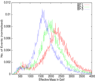
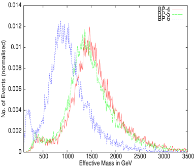
Figure 1: $M_{eff}$ distribution (normalized to unity) of the final state under consideration, for all benchmark points.

      

      

      

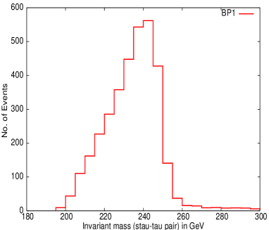
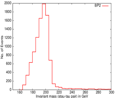
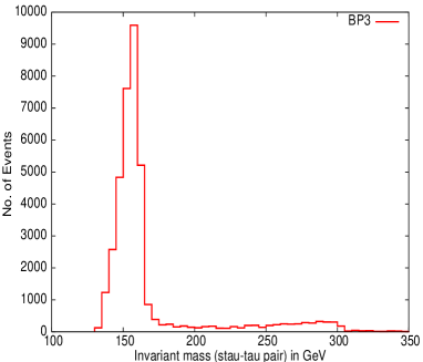
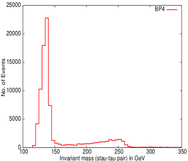
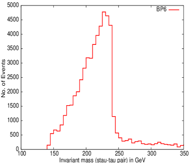
Figure 2: $M_{\tilde{\tau}\tau_{j}}$ distribution for all the benchmark points. BP1, BP2 and BP3 show only the $\chi^{0}_{1}$ peak. Both the $\chi^{0}_{1}$ and $\chi^{0}_{2}$ peaks are visible for BP4 and BP5, while BP6 displays only the $\chi^{0}_{2}$ peak.

Next, for each event that we record, we look at a $\tilde{\tau}$ and a $\tau$-jet of opposite signs. The invariant mass distribution of this $\tilde{\tau}\tau_{j}$ pair displays a peak whose location, although not precisely telling us about the parent neutralino, is still in the vicinity of the mass values. Thus, by observing these distributions (Figure 2) one often is able to tell whether it is a $\chi^{0}_{1}$ or a $\chi^{0}_{2}$, once one simultaneously uses information obtained from the $M_{eff}$ distribution.

As has already been noted in [13], the mass of either $\chi^{0}_{1}$ or $\chi^{0}_{2}$ or both can be reconstructed in this scenario, depending on one’s location in the parameter space. Once a peak in the $\tau\tilde{\tau}$ invariant mass is located, the next step is to check whether $|M_{\tilde{\tau}-\tau_{j}}-m_{\chi^{0}_{i}}|<0.1.m_{\chi^{0}_{i}}$, where $m_{\chi^{0}_{i}}$ is either one (or the only one) of the two lightest neutralinos deemed reconstructible in the corresponding region. The mass of that neutralino is used in equation 9. If this equality is not satisfied for either neutralino or the only one reconstructed, then the event is not included in the analysis.

3.3 SM backgrounds and cuts

The final state we have considered, namely, $\tau_{j}+2\tilde{\tau}{\rm(opposite-sign~{}charged~{}track)}+E_{T}/~{}~{}+X$, suffers from several SM background processes. This is because charged tracks in the muon chamber due to the presence of quasistable charged particle can be faked by muons. Such faking is particularly likely for ultra-relativistic particles, for which neither the time-delay measurement nor the degree of ionisation in the inner tracking chamber is a reliable discriminator. The dominant contributions come from the following subprocesses:

      

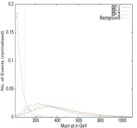
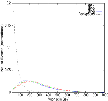
Figure 3: $p_{T}$ distribution (normalised to unity) of the harder muonlike track for the signal and the background, for all benchmark points. The vertical lines indicate the effects of a $p_{T}$-cut at 100 GeV.

      

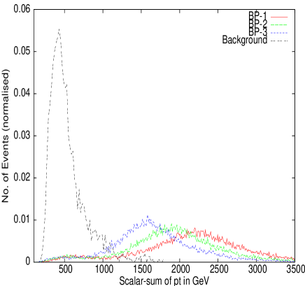
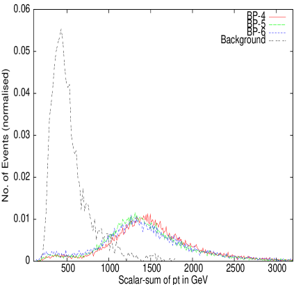
Figure 4: $\Sigma|p_{T}|$ distribution (normalized to unity) for the signal and the background, for all benchmark points.

1. $t\bar{t}$: This is a potential background for any final state in the context of LHC, due to its large production cross-section. In this case $t\bar{t}\rightarrow bW^{+}\bar{b}W^{-}$, followed by various combinations of leptonic as well as hadronic decays of the $b$ and the $W$, can produce opposite sign dimuons and jets. The jets may emanate from actual taus, but may as well be fake. One has an efficiency of 50% in the former case, and a mistagging probability of 1% in the latter. The $t\bar{t}$ cross-section has been multiplied by a K-factor of 1.8 [33].

2. $b\bar{b}$: This, too, has an overwhelmingly large event rate at the LHC. The semileptonic decay of both the b’s ($b\rightarrow c\mu\nu_{\mu}$) can give rise to a dimuon final state and any of the associated jets can be faked as tau-jet. Though the mistagging probability of a non-tau jet being identified as a tau-jet is small, the large cross-section of $b\bar{b}$ production warrants serious attention to this background.

3. $ZZ$: In this case any one of the $Z$’s can decays into a dimuon pair ($Z\rightarrow\mu\mu$) while the other one can decays into $\tau\tau$ pair where only one of the tau can be identified. The hadronic decay of $Z$ and the subsequent misidentification of any of them as tau-jet is also possible.

4. $ZW$: This SM process also contributes to the final state under consideration with $Z\rightarrow\mu\mu$ and $W\rightarrow\tau\bar{\nu}_{\tau}$.

5. $ZH$: This subprocess can also contribute to the final state $\tau_{j}+2\mu(charged-track)+E_{T}/~{}~{}$ where the Higgs decaying into a pair of $\tau$’s, with only one of the $\tau$ being identified has been considered.

Our chosen event selection criteria have been prompted by all the above backgrounds. First of all, we have subjected the events to the following basic cuts:

• $p_{T}^{lep,track}>10$ GeV

• $p_{T}^{hardest-jet}>75$ GeV

• $p_{T}^{other-jets}>30$ GeV

• $40~{}GeV</\!\!\!E_{T}<180~{}GeV$

• $|\eta|<2.5$ for Leptons, Jets & Stau

• $\Delta R_{ll}>0.2,~{}\Delta R_{lj}>0.4$, where $\Delta R^{2}=\Delta\eta^{2}+\Delta\phi^{2}$

• $\Delta R_{\tilde{\tau}l}>0.2,~{}\Delta R_{\tilde{\tau}j}>0.4$

• $\Delta R_{jj}>0.7$

Though the above cuts largely establish the bona fide of a signal event, the background events are too numerous to be effectively suppressed by them. One therefore has to use the fact that the jets and stau-tracks are all arising from the decays of substantially heavy sparticles. This endows them with added degrees of hardness, as compound to jets and muons produced in SM process. Thus we can impose a $p_{T}$ cut on each track on the muon chamber, and also demand a large value of the scalar sum of transverse momenta of all the visible final state particles:

• $p_{T}^{muonlike~{}track}>100~{}GeV$

• $\Sigma|\vec{p_{T}}|>1~{}TeV$

The justification of these cuts can also be seen from Figures 3 and 4. It may be noted that no invariant mass cut on the pair of charged tracks has been imposed. While such a cut, too, can suppress the dimuon background, we find it more rewarding to use the scalar sum of $p_{T}$ cut.

3.4 SUSY backgrounds

Apart from the SM backgrounds, SUSY processes in this scenario itself contribute to the final state $\tau_{j}+2\tilde{\tau}~{}+~{}E_{T}/~{}~{}+X$, which are often more serious than the SM backgrounds. These events will survive the kinematic cuts listed in the previous subsection, since they, too, originate in heavy sparticles produced in the initial hard scattering. The dominant contributions of this kind come from:

1. $\chi^{0}_{i}\chi^{0}_{j}$ production in cascade decay of squarks/gluinos: This is one of the potentially dangerous background where both the $\chi^{0}_{i}$’s ($i,j=1,2$) decay into $\tilde{\tau}\tau$-pairs, with only one tau being identified. This then mimics our final state in all details with a much higher event rate.

2. $\tilde{\nu}_{\tau_{L}}\chi^{0}_{i}$ production in cascade decay of squarks/gluinos: The decay of $\tilde{\nu}_{\tau_{L}}$ as part of the cascade produces a $W\tilde{\tau}_{1}$-pair, while the $\chi^{0}_{i}$ decays into a $\tilde{\tau}\tau$-pair to give rise to same final state with an additional $W$ which then can decay hadronically. The $\tilde{\nu}_{\tau L}$ is produced in association with a tau in large number of events (e.g., $\chi^{\pm}_{1}\rightarrow\tilde{\nu}_{\tau L}\tau$). The $\tilde{\nu}_{\tau_{L}}$ can also be produced from, say, a $\chi^{0}_{2}$. In both of the above situations, a tau-stau pair can be seen together with another stau track, thus leading to a background event.

The first background can be reduced partially by looking at the invariant mass distribution of the $\tilde{\tau}$ (having same sign as that of the identified $\tau$ in the final state) with each jet in the final state. If this distribution for any particular combinations falls within $m_{\chi_{i}}-20<M_{\tilde{\tau}j}<m_{\chi_{i}}+20$ (where $m_{\chi_{i}}=m_{\chi^{0}_{1}}~{}or~{}\frac{m_{\chi^{0}_{2}}}{2}$, depending on whether $\chi^{0}_{1}$ or $\chi^{0}_{2}$ is better constructed), we have thrown away that event. The reason for this lies in the observations depicted in Figure 2; the invariant mass of a $\tau$-induced jet and the $\tilde{\tau}$ which shows a peak close to the mass of the neutralino from which the $\tilde{\tau}$-$\tau$ pair is produced. This has been denoted by Cut X in Tables 2 and 3. In addition, if the available information on the effective mass tells us that the $\chi^{0}_{2}$ is better reconstructed in the region, and is produced along with a $\chi^{0}_{1}$ with substantial rate, then a similar invariant mass cut around the $\chi^{0}_{2}$ mass will also be useful. A further cut on the transverse mass distribution $M^{T}_{\tilde{\tau}\nu_{\tau}}$ ($>1.5m_{\chi^{0}_{1}}$ or $0.75m_{\chi^{0}_{2}}$) substantially decreases this background without seriously effecting the signal.

The background of the second kind can in principle be reduced by vetoing events with additional $W$’s. To identify events with $W$ we have considered only the hadronic decays of $W$’s. We first observe the $\Delta R$ separation between the stau (produced in decay of $\tilde{\nu}_{\tau L}$) and the direction formed out of the vector sum of the momenta of the two jets produced in $W$ decay. If this separation lies within $\Delta R=0.8$ and the invariant mass of the two jets lies within $M_{W}-20<M_{jj}<M_{W}+20$ we discard that particular event. In addition, for a sufficiently boosted $W$, one can have a situation where the two jets merge to form a single jet. For such a case, we again look at the stau and each jet within $\Delta R<0.8$ around it. The invariant mass of the resultant jet is taken to be 20% of the jet energy. The event is rejected if a jet with the mass lies within $\pm$20 GeV of the $W$-mass. We have denoted this by Cut Y in Tables 2 and 3. Of course, while it is useful in reducing the background, a fraction of the signal events also gets discarded in the process.

4 Numerical results

We finally present the numerical results of our study, after imposing the various cuts for all the benchmark points. From Tables 2 and 3 one can see that, after demanding a minimum hardness of the charged track ($p^{track}_{T}>100$ GeV), together with the cut on the scalar sum of $p_{T}$ ($\Sigma|p_{T}|>1TeV$), the contribution from the SM processes get reduced substantially. The cuts X and Y, defined in the previous subsection, are relatively inconsequential for SM processes. However, in the process of solving for neutrino momentum in tau decay, most of the SM background events gets eliminated on demanding the invariant mass of the tau, paired with a oppositely charged track, to be around the neutralino mass ($m_{\chi^{0}_{1}}~{}or~{}m_{\chi^{0}_{2}}$). This is due to the demand that the solution be physical, i.e. the fraction $x$ lies between 0 and 1. It is very unlikely to have admissible solutions for $x$ in SM processes, with the $\tau$-(muon)track pair invariant mass peaking at $m_{\chi^{0}_{1}}$/$m_{\chi^{0}_{2}}$. Thus, although the demand $0<x<1$ is not meant specifically for background elimination, it is nonetheless helpful in reducing backgrounds. We have verified that the SM contributions within a bin of $\pm 20$GeV around the reconstructed peak is very small.

As has been already mentioned, SUSY backgrounds within the model itself is hard to get rid of completely. The peak in the transverse mass distribution of the $\tilde{\tau}$-$\nu_{\tau}$ pair get smeared due to such background events (see Figure 4). We have already mentioned two suggested cuts, namely, X and Y, which partially reduce these backgrounds. Of these, cut Y suppresses (by about 15%) some of the $\tilde{\nu}_{\tau_{L}}$-$\chi^{0}_{1/2}$ events, as can be seen from Tables 2 and 3. the effects of this cut on the other SUSY backgrounds as well as the signal are very similar.

Cut X, meant to eliminate mainly the $\chi^{0}_{i}$-$\chi^{0}_{j}$ background. Our analysis shows that this cut is rather effective in in this respect; the event rate is reduced by almost 50% Surprisingly, it also reduces the $\tilde{\nu}_{\tau_{L}}$-$\chi^{0}_{1/2}$ background by a considerable amount. The reason for this is the following: $\tilde{\nu}_{\tau_{L}}$-$\chi^{0}_{1/2}$ is produced in cascade decays of squarks and gluinos and the $\tilde{\nu}_{\tau_{L}}$ is often produced from a $\chi^{\pm}_{1}$ (the branching fraction being 30% or more in some BP’s). In that case the decay process is $\chi^{\pm}_{1}\rightarrow\tau^{\pm}\tilde{\nu}_{\tau_{L}}$. The tau out of such a $\chi^{\pm}_{1}$ is sometimes identified, whereas the tau out of a $\chi^{0}_{1/2}$ ($\chi^{0}_{1/2}\rightarrow\tau^{\pm}\tilde{\tau}^{\mp}$) from the other decay chain goes untagged. The invariant mass distribution of a track and the jet coming from an unidentified $\tau$ is clustered around $m_{\chi^{0}_{i}}$ ($i$ = 1,2). Thus cut X turns out to be effective in eliminating this type of background.

After all this effort, however, one still left with background events which smear the peak in the transverse mass distribution of the $\tilde{\tau}\nu_{\tau}$-pair. We have to impose an aadditional cut on the transverse mass distribution to separate the peak from the background event. This is in the form of the demand $M^{T}_{\tilde{\tau}\nu_{\tau}}>\frac{3}{4}m_{\chi^{0}_{2}}$, whereby it is possible to reduce these backgrounds further, as can be seen from Tables 2 and 3. It is then possible to determine the chargino mass ($m_{\chi^{\pm}_{1}}$) by looking at the peak, followed by a sharp descent, in the transverse mass distribution for several benchmark points.

The transverse mass distributions for different benchmark points are shown in Figures 5 and 6. The tau-identification efficiency is assumed to be 50% in Figure 5; Figure 6 reflects the improvement achieved in a relatively optimistic situation when this efficiency is 70%.

BP1	Signal	SM	SUSY backgrounds
	($\chi^{0}_{1/2}-\chi^{\pm}_{1}$)	backgrounds	$\chi^{0}_{1}-\chi^{0}_{1}$	$\chi^{0}_{1}-\chi^{0}_{2}$	$\chi^{0}_{2}-\chi^{0}_{2}$	$\chi^{0}_{1/2}-\tilde{\nu}_{\tau L}$
Basic cuts	121	65588	2557	62	1	786
With $p_{T}$+$\Sigma{|p_{T}|}$ Cut	92	202	2236	49	1	551
Cut Y	83	202	1969	42	1	433
Cut X	58	202	1130	26	1	244
$M^{T}_{\tilde{\tau}\nu_{\tau}}>\frac{3}{4}m_{\chi^{0}_{2}}$	28	10	83	2	0	25
$|M_{peak}-M^{T}_{\tilde{\tau}\nu_{\tau}}|\leq 20$	9	3	7	0	0	2
BP2	Signal	SM	SUSY backgrounds
	($\chi^{0}_{1/2}-\chi^{\pm}_{1}$)	backgrounds	$\chi^{0}_{1}-\chi^{0}_{1}$	$\chi^{0}_{1}-\chi^{0}_{2}$	$\chi^{0}_{2}-\chi^{0}_{2}$	$\chi^{0}_{1/2}-\tilde{\nu}_{\tau L}$
Basic cuts	677	65588	6600	390	9	2157
With $p_{T}$+$\Sigma{|p_{T}|}$ Cut	492	202	5552	301	7	1418
Cut Y	444	202	4885	262	6	1106
Cut X	336	202	2675	170	5	605
$M^{T}_{\tilde{\tau}\nu_{\tau}}>\frac{3}{4}m_{\chi^{0}_{2}}$	173	3	278	26	1	76
$|M_{peak}-M^{T}_{\tilde{\tau}\nu_{\tau}}|\leq 20$	62	0	33	5	0	11
BP3	Signal	SM	SUSY backgrounds
	($\chi^{0}_{1/2}-\chi^{\pm}_{1}$)	backgrounds	$\chi^{0}_{1}-\chi^{0}_{1}$	$\chi^{0}_{1}-\chi^{0}_{2}$	$\chi^{0}_{2}-\chi^{0}_{2}$	$\chi^{0}_{1/2}-\tilde{\nu}_{\tau L}$
Basic cuts	5519	65588	19400	3361	170	6959
With $p_{T}$+$\Sigma{|p_{T}|}$ Cut	3571	202	15181	2240	98	4186
Cut Y	3131	202	13091	1924	91	3231
Cut X	2372	202	6974	1192	71	1679
$M^{T}_{\tilde{\tau}\nu_{\tau}}>\frac{3}{4}m_{\chi^{0}_{2}}$	1189	0	985	205	14	208
$|M_{peak}-M^{T}_{\tilde{\tau}\nu_{\tau}}|\leq 20$	523	0	154	46	1	27

Table 2: Number of signal and background events for the $\tau_{j}+2\tilde{\tau}$ (charged-track)+$E_{T}/~{}~{}+X$ final state, considering all SUSY processes, for BP1, BP2 and BP3 at an integrated luminosity 300 $fb^{-1}$ assuming tau identification efficiency $\epsilon_{\tau}=50\%$.

BP4	Signal	SM	SUSY backgrounds
	($\chi^{0}_{1/2}-\chi^{\pm}_{1}$)	backgrounds	$\chi^{0}_{1}-\chi^{0}_{1}$	$\chi^{0}_{1}-\chi^{0}_{2}$	$\chi^{0}_{2}-\chi^{0}_{2}$	$\chi^{0}_{1/2}-\tilde{\nu}_{\tau L}$
Basic cuts	18194	65588	33076	10618	886	10613
With $p_{T}$+$\Sigma{|p_{T}|}$ Cut	10697	202	24475	6342	439	5713
Cut Y	9431	202	21100	5431	368	4436
Cut X	4875	202	7583	2132	157	1480
$M^{T}_{\tilde{\tau}\nu_{\tau}}>\frac{3}{4}m_{\chi^{0}_{2}}$	2345	0	1274	439	41	231
$|M_{peak}-M^{T}_{\tilde{\tau}\nu_{\tau}}|\leq 20$	1076	0	254	114	13	58
BP5	Signal	SM	SUSY backgrounds
	($\chi^{0}_{1/2}-\chi^{\pm}_{1}$)	backgrounds	$\chi^{0}_{1}-\chi^{0}_{1}$	$\chi^{0}_{1}-\chi^{0}_{2}$	$\chi^{0}_{2}-\chi^{0}_{2}$	$\chi^{0}_{1/2}-\tilde{\nu}_{\tau L}$
Basic cuts	34489	65588	39521	19574	1976	12039
With $p_{T}$+$\Sigma{|p_{T}|}$ Cut	18748	202	28329	10827	958	5953
Cut Y	16419	202	24348	9326	815	4586
Cut X	8508	186	8869	3764	376	1626
$M^{T}_{\tilde{\tau}\nu_{\tau}}>\frac{3}{4}m_{\chi^{0}_{2}}$	4099	0	1574	866	144	258
$|M_{peak}-M^{T}_{\tilde{\tau}\nu_{\tau}}|\leq 20$	2145	0	339	221	52	37
BP6	Signal	SM	SUSY backgrounds
	($\chi^{0}_{1/2}-\chi^{\pm}_{1}$)	backgrounds	$\chi^{0}_{1}-\chi^{0}_{1}$	$\chi^{0}_{1}-\chi^{0}_{2}$	$\chi^{0}_{2}-\chi^{0}_{2}$	$\chi^{0}_{1/2}-\tilde{\nu}_{\tau L}$
Basic cuts	17146	65588	14519	20756	1970	4644
With $p_{T}$+$\Sigma{|p_{T}|}$ Cut	8379	202	9593	11405	968	2524
Cut Y	7326	202	8004	9776	778	2025
Cut X	4204	186	3837	5697	374	1038
$M^{T}_{\tilde{\tau}\nu_{\tau}}>\frac{3}{4}m_{\chi^{0}_{2}}$	1475	0	231	1783	128	15
$|M_{peak}-M^{T}_{\tilde{\tau}\nu_{\tau}}|\leq 20$	774	0	62	569	44	0

Table 3: Same as in Table-2, but for BP4, BP5 and BP6.

      

      

      

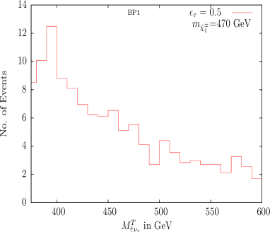
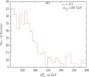
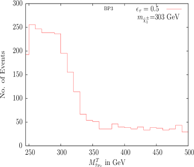
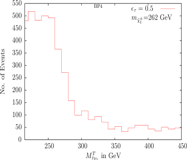
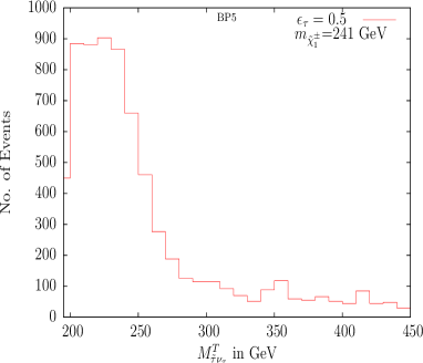
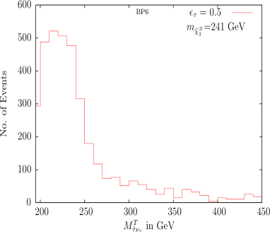
Figure 5: The transverse mass $\tilde{\tau}\nu_{\tau}$-pair from chargino deacy described in the text, for all the benchmark points with tau identification efficiency $(\epsilon_{\tau})=50\%$.

      

      

      

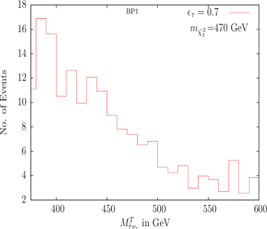
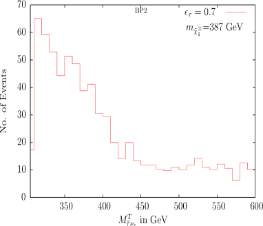
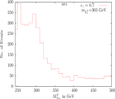
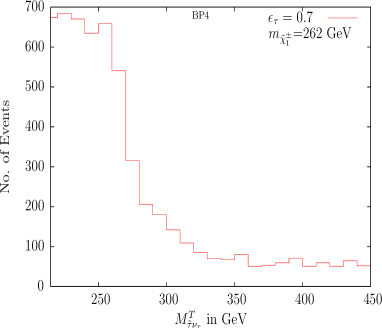
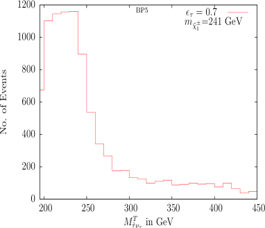
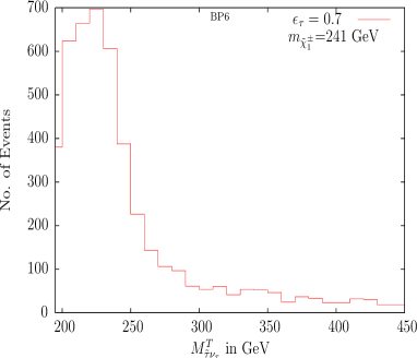
Figure 6: Same as in Figure 5, but with tau identification efficiency $(\epsilon_{\tau})=70\%$.

At BP1 the statistics is very poor and we have realtively few events within a bin of 40 GeV around $m_{\chi^{\pm}_{1}}$. One has about 50% of the events coming from other SUSY processes (Table 2). Also the peak is not clearly visible due to the presence of a large number of $\chi^{0}_{1}\chi^{0}_{1}$ events, even after imposing the $M^{T}_{\tilde{\tau}\nu_{\tau}}$ $>\frac{3}{4}m_{\chi^{0}_{2}}$ cut.

The situation is similar for BP2 as well. In BP3 and BP4 the peak followed by a sharp fall is considerably more distinct, from which one can extract the value of $m_{\chi^{\pm}_{1}}$.

For BP5 and BP6 the contamination due to the SUSY background is found to be small compared to the other benchmark points.

The $\chi^{\pm}_{1}$ production rate in cascade decays of squarks/gluinos is also higher there. Hence the transverse mass distribution shows a distinct peak, from which a faithful reconstruction of chargino mass is possible.

As a comparison between Figures 5 and 6 shows, the prospect can be improved noticeably if one has a better tau identification efficiency ($\epsilon_{\tau}=70\%$). In such a case, the background from $\chi^{0}_{1}$-$\chi^{0}_{1}$/$\chi^{0}_{1}$-$\chi^{0}_{2}$/$\chi^{0}_{2}$-$\chi^{0}_{2}$ is less severe compared to the case where the tau identification efficiency is 50%.

From Figures 5 and 6, one can also see some small peaks in the $M^{T}_{\tilde{\tau}\nu_{\tau}}$ distribution with very few event rate, in the region where $M^{T}_{\tilde{\tau}\nu_{\tau}}>m_{\chi^{0}_{2}}$. This can be attributed to those events where a $\chi^{0}_{3}$ or a $\chi^{0}_{4}$ decays into a $\tilde{\tau}\tau$ pair, and also to the production of the heavier chargino.

5 Summary and conclusions

We have considered a SUSY scenario where the LSP is dominated by a right-sneutrino state, while a dominantly right-chiral stau is the NLSP. The stau, being stable on the length scale of collider detectors, gives rise to charged tracks, the essence of SUSY signal in such a scenario. It is also shown that such a spectrum follows naturaly from a high-scale scenario of universal scalar and gaugino masses.

We have extended our earlier study on the mass reconstruction of non-strongly interacting superparticles in such cases, by considering final states resulting from the decays of a $\chi^{\pm}_{1}\chi^{0}_{1(2)}$ pair in SUSY cascades. The final state under consideration is $\tau_{j}+2\tilde{\tau}{\rm(opposite-sign~{}charged~{}tracks)}+E_{T}/~{}~{}+X$. We have systematically developed a procedure for identifying the contribution to $\vec{p_{T}/~{}~{}}$ from the neutrino produced in $\chi^{\pm}_{1}$-decay, together with a quasi-stable stau. Once this is possible, the transverse mass distribution of the corresponding $\tilde{\tau}-\nu_{\tau}$ pair can be extracted from data at the LHC, and a sharp edge in that distribution yields information on the chargino mass. While eliminating the SM backgrounds in this process is straightforward, we have suggested ways of minimising the contamination of the relevant final state from competing processes in the same SUSY scenario. Selecting a number of benchmark points in the parameter space, we show in which regions the above procedure works. In cases where it does not, the main causes of failure are identified as the overwhelmingly large contribution from $\chi^{0}_{1}$-pairs, and, for example, in the first two benchmark points, somewhat poor statistics. The other important issue is the differentiation between the $\chi^{0}_{1}$ and the $\chi^{0}_{2}$ produced in association with the $\chi^{\pm}_{1}$. For this, we make use of the assumption of gaugino universality as well as the information extacted from the effective mass distribution in SUSY processes.

To conclude, the existence of quasi-stable charged particles, a possibility not too far-fetched, opens a new vista in the reconstruction of superparticle masses. We have repeatedly suggested utilisation of this facility in our works on gluino[6] and neutralino[13] mass reconstruction. The present work underscores a relatively arduous task in this respect, in obtaining transverse mass edges in chargino decays. In spite of rather challenging obstacles from underlying SUSY processes, we demonstrate the feasibility of our procedure, which is likely to be enhanced by improvement in, for example, the W-and tau-identification efficiencies.

Acknowledgment: This work was partially supported by funding available from the Department of Atomic Energy, Government of India for the Regional Centre for Accelerator-based Particle Physics, Harish-Chandra Research Institute. Computational work for this study was partially carried out at the cluster computing facility of Harish-Chandra Research Institute (http://cluster.mri.ernet.in).

References

- [1] For reviews see for example, H. E. Haber and G. L. Kane, Phys. Rept. 117, 75 (1985).
- [2] S. Dawson, E. Eichten and C. Quigg, Phys. Rev. D 31, 1581 (1985); X. Tata, arXiv:hep-ph/9706307. M. E. Peskin, arXiv:0801.1928 [hep-ph].
- [3] K. Hamaguchi, M. M. Nojiri and A. de Roeck, JHEP 0703, 046 (2007) [arXiv:hep-ph/0612060].
- [4] T. Schwetz, M. Tortola and J. W. F. Valle, New J. Phys. 10, 113011 (2008) [arXiv:0808.2016 [hep-ph]]. G. L. Fogli et al., Phys. Rev. D 78, 033010 (2008) [arXiv:0805.2517 [hep-ph]]. A. Bandyopadhyay, S. Choubey, S. Goswami, S. T. Petcov and D. P. Roy, arXiv:0804.4857 [hep-ph].
- [5] C. L. Chou and M. E. Peskin, Phys. Rev. D 61, 055004 (2000) [arXiv:hep-ph/9909536].
- [6] D. Choudhury, S. K. Gupta and B. Mukhopadhyaya, Phys. Rev. D 78, 015023 (2008) [arXiv:0804.3560 [hep-ph]].
- [7] S. K. Gupta, B. Mukhopadhyaya and S. K. Rai, Phys. Rev. D 75, 075007 (2007) [arXiv:hep-ph/0701063].
- [8] A. H. Chamseddine, R. L. Arnowitt and P. Nath, Phys. Rev. Lett. 49 (1982) 970.
- [9] M. Kawasaki, K. Kohri and T. Moroi, Phys. Lett. B 649, 436 (2007) [arXiv:hep-ph/0703122].
- [10] C. Amsler et al. [Particle Data Group], Phys. Lett. B 667, 1 (2008).
- [11] E. Komatsu et al. Astrophys. J. Suppl. 180, 330 (2009) [arXiv:0803.0547 [astro-ph]].
- [12] T. Asaka, K. Ishiwata and T. Moroi, Phys. Rev. D 73, 051301 (2006) [arXiv:hep-ph/0512118]. T. Asaka, K. Ishiwata and T. Moroi, Phys. Rev. D 75, 065001 (2007) [arXiv:hep-ph/0612211].
- [13] S. Biswas and B. Mukhopadhyaya, Phys. Rev. D 79, 115009 (2009) [arXiv:0902.4349 [hep-ph]].
- [14] J. Smith, W. L. van Neerven and J. A. M. Vermaseren, Phys. Rev. Lett. 50, 1738 (1983).
- [15] J. L. Feng, A. Rajaraman and F. Takayama, Phys. Rev. Lett. 91, 011302 (2003) [arXiv:hep-ph/0302215]; J. L. Feng, A. Rajaraman and F. Takayama, Phys. Rev. D 68, 063504 (2003) [arXiv:hep-ph/0306024]; J. R. Ellis, K. A. Olive, Y. Santoso and V. C. Spanos, Phys. Lett. B 588, 7 (2004) [arXiv:hep-ph/0312262]; J. L. Feng, S. Su and F. Takayama, Phys. Rev. D 70, 075019 (2004) [arXiv:hep-ph/0404231]; A. Ibarra and S. Roy, JHEP 0705, 059 (2007) [arXiv:hep-ph/0606116].
- [16] S. Dimopoulos, M. Dine, S. Raby and S. D. Thomas, Phys. Rev. Lett. 76, 3494 (1996) [arXiv:hep-ph/9601367]. D. A. Dicus, B. Dutta and S. Nandi, Phys. Rev. Lett. 78, 3055 (1997) [arXiv:hep-ph/9701341]; S. Ambrosanio, G. D. Kribs and S. P. Martin, Phys. Rev. D 56, 1761 (1997) [arXiv:hep-ph/9703211]; D. A. Dicus, B. Dutta and S. Nandi, Phys. Rev. D 56, 5748 (1997) [arXiv:hep-ph/9704225]; K. M. Cheung, D. A. Dicus, B. Dutta and S. Nandi, Phys. Rev. D 58, 015008 (1998) [arXiv:hep-ph/9711216]; J. L. Feng and T. Moroi, Phys. Rev. D 58, 035001 (1998) [arXiv:hep-ph/9712499]; P. G. Mercadante, J. K. Mizukoshi and H. Yamamoto, Phys. Rev. D 64, 015005 (2001) [arXiv:hep-ph/0010067].
- [17] A. V. Gladyshev, D. I. Kazakov and M. G. Paucar, Mod. Phys. Lett. A 20, 3085 (2005) [arXiv:hep-ph/0509168]; T. Jittoh, J. Sato, T. Shimomura and M. Yamanaka, Phys. Rev. D 73, 055009 (2006) [arXiv:hep-ph/0512197].
- [18] S. P. Martin, arXiv:hep-ph/9709356, and references therein;
- [19] S. P. Martin and P. Ramond, Phys. Rev. D 48 (1993) 5365 [arXiv:hep-ph/9306314].
- [20] N. Arkani-Hamed, L. J. Hall, H. Murayama, D. Tucker-Smith and N. Weiner, Phys. Rev. D 64, 115011 (2001) [arXiv:hep-ph/0006312].
- [21] D. L. Rainwater, D. Zeppenfeld and K. Hagiwara, Phys. Rev. D 59, 014037 (1998) [arXiv:hep-ph/9808468].
- [22] G. Aad et al. [The ATLAS Collaboration], [arXiv:0901.0512].
- [23] F. E. Paige, S. D. Protopopescu, H. Baer and X. Tata, arXiv:hep-ph/0312045.
- [24] A. Djouadi, M. Drees and J. L. Kneur, JHEP 0603, 033 (2006) [arXiv:hep-ph/0602001].
- [25] T. Sjostrand, S. Mrenna and P. Skands, JHEP 0605, 026 (2006) [arXiv:hep-ph/0603175].
- [26] H. L. Lai et al. [CTEQ Collaboration], Eur. Phys. J. C 12, 375 (2000) [arXiv:hep-ph/9903282].
- [27] W. Beenakker, R. Hopker, M. Spira and P. M. Zerwas, Nucl. Phys. B 492, 51 (1997) [arXiv:hep-ph/9610490].
- [28] C. G. Lester and D. J. Summers, Phys. Lett. B 463, 99 (1999) [arXiv:hep-ph/9906349].
- [29] B. Gripaios, JHEP 0802, 053 (2008) [arXiv:0709.2740 [hep-ph]]; H. C. Cheng and Z. Han, JHEP 0812, 063 (2008) [arXiv:0810.5178 [hep-ph]]; A. J. Barr, B. Gripaios and C. G. Lester, arXiv:0908.3779 [hep-ph].
- [30] Y. Coadou et al. ATLAS Internal Note ATL-PHYS-98-126
- [31] The CMS Collaboration, CMS-TDR-8.1, CERN/LHCC 2006-001
- [32] S. Asai et al., Eur. Phys. J. C 32S2, 19 (2004) [arXiv:hep-ph/0402254].
- [33] W. Beenakker, S. Dittmaier, M. Kramer, B. Plumper, M. Spira and P. M. Zerwas, Nucl. Phys. B 653, 151 (2003) [arXiv:hep-ph/0211352].