HD 174884: a strongly eccentric, short-period early-type binary system discovered by CoRoT

Accurate photometric CoRoT space observations of a secondary seismological target, HD 174884, led to the discovery that this star is an astrophysically important double-lined eclipsing spectroscopic binary in an eccentric orbit ($e\sim 0.3$), unusual for its short 3$\aas@@fstack{d}$65705 orbital period. The high eccentricity, coupled with the orientation of the binary orbit in space, explains the very unusual observed light curve with strongly unequal primary and secondary eclipses having the depth ratio of 1-to-100 in the CoRoT “seismo” passband. Without the high accuracy of the CoRoT photometry, the secondary eclipse, 1.5 mmag deep, would have gone unnoticed. A spectroscopic follow-up program provided 45 high dispersion spectra. The analysis of the CoRoT light curve was performed with an adapted version of PHOEBE that supports CoRoT passbands. The final solution was obtained by simultaneous fitting of the light and the radial velocity curves. Individual star spectra were derived by spectrum disentangling. The uncertainties of the fit were derived by bootstrap resampling and the solution uniqueness was tested by heuristic scanning.

The results provide a consistent picture of the system composed of two late B stars. The Fourier analysis of the light curve fit residuals yields two components, with orbital frequency multiples and an amplitude of $\sim$ 0.1 mmag, which are tentatively interpreted as tidally induced pulsations.

An extensive comparison with theoretical models is carried out by means of the Levenberg-Marquardt minimization technique and the discrepancy between models and the derived parameters is discussed. The best fitting models yield a young system age of 125 million years which is consistent with the eccentric orbit and synchronous component rotation at periastron.

1 Introduction

HD 174884 (Corot 7758) was selected as a seismology target for the first short run in the CoRoT “center” direction (SRc1) because – on the basis of its B8 V spectral classification – it was considered a good candidate to pinpoint the instability strip red edge of the Slowly Pulsating B stars (e.g. Waelkens et al. 1998). Its only available spectrum, obtained before launch with the Elodie spectrograph and available from the Gaudi database (Solano et al. 2005) did not reveal the star’s binary nature, which was instead immediately evident from CoRoT photometry. The system was continuously observed during 27 days. The light curve of HD 174884 is characterized by signatures of high eccentricity: the secondary minimum markedly displaced from phase 0.5 and a bump, typical of close eccentric binaries, due to variable distortion of stellar surfaces along the orbit. The system is very interesting for several reasons: the high eccentricity is coupled with quite short a period ($P_{orb}=3\aas@@fstack{d}66$), putting the system in an extreme location of the period - eccentricity diagram of B stars. This indicates young age or an inefficient circularization process. Secondly, the huge difference between the primary and secondary minima, the latter detected only thanks to CoRoT accuracy, and the overall shape and accuracy of the light curve is a challenge for light curve fitting methods and a test of their adequacy to solve light curves of this unprecedented quality. Finally, only a thorough analysis of HD 174884 could yield information of the possible pulsational properties of the components.

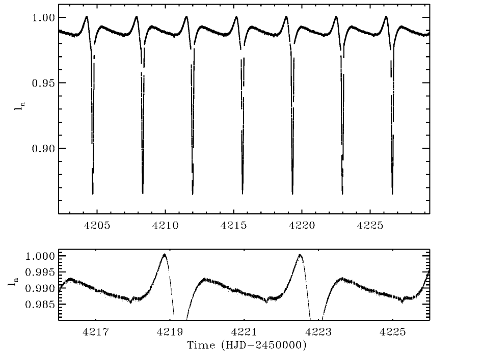
Figure 1: Upper panel: the complete CoRoT light curve of HD 174884 as normalized flux vs HJD. Lower panel: a blow-up, spanning approximately three periods, showing the tiny secondary minimum (first occurrence at reduced HJD of around 4218)

In the following sections we present the results of the analysis of CoRoT photometry and of ground-based high dispersion spectroscopy. A critical analysis of parameter uncertainties and of the uniqueness of the light and radial velocity curve solution is an essential part of the study.

The well constrained physical parameters of the binary components are then compared with evolutionary models computed with the CLÉS code (Code Liègeois d’ Évolution Stellaire, Scuflaire et al. 2008b) with the aim of constraining the age and the structural parameters (chemical composition, overshooting). Finally the light curve fit residuals, with variations of a few $10^{-4}$ mag, are analyzed.

2 Observations of HD 174884 and their analysis

2.1 CoRoT photometry and extant data

HD 174884 is a relatively bright star and several photometric measurements could be found in databases and catalogs. A spectral classification as B8 V appears in the Simbad database (operated at CDS, Strasbourg, France) and was confirmed by the Gaudi classification. Available magnitudes and colors are collected in Table 1, the Strömgren photometry is from the Gaudi database, the infrared ones from 2MASS (Skrutskie et al. 2006). These magnitudes and colors were dereddened according to Moon (1985), assuming a ratio of total to selective absorption $A_{\mathrm{v}}/E(b-y)=4.28$ (Crawford & Mandwewala 1976). For the 2MASS colors the respective ratios were taken from Rieke & Lebofsky (1985). The colors, once corrected for the rather heavy absorption, correspond to the expected values for the (primary) spectral type, and in particular rule out the presence of a near IR excess,which was suggested by the observed values. The star was also observed by Hipparcos, but its parallax is of little use, being affected by a large error, $\pi=1.95\pm 0.73$ mas, according to the new reduction of the Hipparcos data (van Leeuwen 2007).

Table 1: Colors and magnitudes of HD 174884

	Observed	Dereddened
V	7.998$\pm$0.002	7.001 $\pm$0.006
b-y	0.173$\pm$0.001	-0.055$\pm$0.002
m1	0.042 $\pm 0.001$	0.117$\pm$0.001
c1	0.637$\pm$0.005	0.594$\pm$0.005
$\beta$	2.701 $\pm$0.011
J	7.577$\pm$ 0.024	7.302$\pm$0.025
H	7.562$\pm$ 0.023	7.391 $\pm$ 0.024
K	7.521$\pm$ 0.021	7.412$\pm$0.021

CoRoT observed HD 174884 (Corot ID: 7758) for 27 days. The almost uninterrupted time series extends over about seven orbital cycles with a time sampling of $32^{\mathrm{s}}$. The full light curve has 60016 points, after removal of the measurements perturbed by South Atlantic Anomaly crossing (proton events). Each point is the mean made of 32 1-s exposures and has, therefore, an associated r.m.s. deviation, which is typically of the order of $10^{-3}$ times the measured flux.

A slow decreasing trend, presumably due to some kind of instrumental decay or gradual pointing drift, was corrected by fitting and subtracting a second order polynomial passing through the maxima. Furthermore, we deleted a few hundred spurious points that arise from the inadequate linear fit used in the first version of the CoRoT pipeline. The complete, normalized, light curve (59492 points) is shown in Fig. 1 together with a blow-up of the central part, displaying a tiny ($\simeq 1.5$ mmag deep) secondary minimum.

The binary period was derived in two steps: an initial estimate with Period04 (Lenz & Breger 2005) was refined with the Phase Dispersion Minimization method (Stellingwerf 1978), which is better suited for the analysis of non-sinusoidal variations. The epoch of primary minimum was derived by a linear fit to the seven minimum epochs, which were obtained by parabolic fit to the curve minima. The results were checked with PHOEBE (Prša & Zwitter 2005). Note that PHOEBE determines the epoch of zero phase with respect to the argument of periastron (rather than with the position of the primary minimum), and provides phases for important positions in orbit, like superior conjunction. We adopt the following ephemeris:

$$T_{\mathrm{minI}}=2454204.68162(4)+3\aas@@fstack{d}65705(1)\times E.$$ (1)

The light curve was folded with this period and found to be stable within the observed time frame, as the dispersion of the phased curve was comparable to that of the original time series. Therefore, we binned the oversampled curve into 650 normal points, to facilitate the light curve solution. The binning was performed with a variable step, $\Delta\phi=0.002$ outside the eclipses and $\Delta\phi=0.0005$ during the eclipses to keep good sampling. The mean number of points contributing to normals is $\sim 130$ outside the eclipse and $\sim 30$ inside, the folded light curve is shown in Fig. 2.

2.1.1 Preliminary light curve analysis

Figure 2: Upper panel: the phased and binned CoRoT light curve of HD 174884. Dots: normal points as described in the text. The solid line is the light curve fit according to the model of Sect. 3, which can be distinguished from normal points only during primary eclipse. Lower panel: the corresponding residuals (observed - computed normalized flux)

The light curve fit procedure went through several stages, also because the spectroscopic data were obtained only some months after the CoRoT run, thanks to a follow-up program organized after the discovery of binarity. Our final fit is a simultaneous solution of both light and radial velocity curves, but the first steps, based on photometry alone, were quite instructive. They were a test of what can be derived from a single light curve which, on the one side, is of unprecedented accuracy but on the other has features suggesting weak constraining of the solution.

All light curve solutions were performed with PHOEBE (Prša & Zwitter 2005), which was expanded to include flux computation in the CoRoT passbands for both seismology and exo-planet field. Specific passband intensities and limb darkening coefficients were computed for CoRoT passbands from Castelli & Kurucz (2004)’s NEWODF models spanning from 3500 K to 50,000 K across the entire H-R diagram. The spectral energy distribution functions (SEDs) were synthesized with SPECTRUM 2.75 (Gray & Corbally 1994) at a 1 Å dispersion, on a 3000 Å to 10,000 Å  wavelength range. The limb darkening tables were computed by synthesizing SEDs in 20 values of $\mu=\cos\theta$ from the center of the disk to the limb, and fitting the linear cosine law and non-linear log and square root laws by least squares.

For the preliminary solutions, we profited from the scripter version of PHOEBE and used Nelder & Mead’s Simplex minimization for quick descent towards the minima and standard differential corrections when close to the solution. The value of primary effective temperature was fixed to that provided by Gaudi, which is derived by means of the code TempLogG and Strömgren photometry. TempLogG uses the grids of Moon & Dworetsky (1985) in the $T_{\rm eff}$-log g parameter space, with the improvements by Napiwotzki et al. (1993). The resulting value is $T_{\mathrm{eff,1}}=13140$ K; we did not use the internal error from TempLogG but assumed an uncertainty of 1500 K, expressing the accuracy of $T_{\rm eff}$ determination for B-stars by different methods (De Ridder et al. 2004). For the secondary star we actually started from a $T{\rm eff}$ value (3500 K) very far from the final one (wrongly) assuming, on the basis of the great difference of in-eclipse depths, a small, cool secondary star.

We computed, as starting value of a grid, pairs of eccentricity ($e$) and longitude of periastron ($\omega$) providing the observed distance between maxima. The parameters adjusted in the minimizations were inclination $i$, $e$, $\omega$, $T_{\mathrm{eff,2}}$, and surface potentials $\Omega_{1,2}$; the primary passband luminosity $L_{1}$ was separately computed, rather than adjusted, as this allows a smoother convergence to the minimum (Prša & Zwitter 2005). For limb darkening we adopted a square root law that employs two coefficients, $x_{LD}$ and $y_{LD}$ per star and per passband. The gravity darkening and albedo coefficients were kept fixed at their theoretical values, $g=1.0$ and $A=1.0$ for radiative envelopes (von Zeipel 1924). The mass ratio was set to values between 0.1 and 0.5. When the adjustment of these parameters did not provide further improvement, we attempted to adjust synchronicity parameters (ratios of rotational to orbital velocity), $F_{1,2}$.

In spite of the very shallow secondary eclipse and the low inclination, the solution we obtained is fairly close to the final one, implying that the single light curve is already constraining the solution (this was confirmed later on by the results of heuristic scan, presented in Section 3.3). In particular, we could exclude solutions with a cool secondary, in favour of a system configuration yielding a grazing eclipse of a relatively hot secondary star. The very different depth of eclipses is actually due to the combination of high eccentricity and orbit orientation in space.

It was interesting to check, a posteriori, that this single light curve solution gave the following deviations for the various parameters with respect to the combined solution of photometry and radial velocity data: 6% for $e$ and $\omega$, 1% for $i$, 15% for $T_{\mathrm{eff,2}}$, 6-15% for the component radii ($r{{}_{\mathrm{1}}}$,$r{{}_{\mathrm{2}}}$), 12% on $L_{1}$. We did not adjust the mass ratio, and actually the true value is outside the range we explored, but we had indeed a tendency of smaller values of the cost function for the higher $q$ values. Furthermore, the value of $F_{1}$ was within 7% of that derived later on from line profile fitting. On the other hand the value of $F_{2}$ was almost 4 times the spectroscopic one.

In conclusion the light curve solution was well constrained for the main parameters and for primary rotational distortion. This has to be put in relation to the high eccentricity signatures which act as pinpoints on the parameter values.

Table 2: Radial velocities of HD 174884

BJD -245000	$v_{\mathrm{rad,1}}$	$v_{\mathrm{rad,2}}$
	(km s-1)	(km s-1)
4625.6910668	-94.5 $\pm$1.6	85.1$\pm$2.6
4625.7333949	-97.1 $\pm$1.7	87.6$\pm$2.6
4625.7767647	-97.5 $\pm$1.5	99.5 $\pm$2.5
4625.8241393	-104.4$\pm$1.5	99.3$\pm$2.5
4625.8549044	-107.6$\pm$1.5	99.0$\pm$2.5
4626.6823677	-78.7 $\pm$1.6	69.8$\pm$2.7
4626.7347772	-74.8 $\pm$1.6	63.9$\pm$2.7
4626.7602527	-76.1 $\pm$1.6	60.4$\pm$2.7
4626.7880894	-74.4 $\pm$1.6	58.2$\pm$2.8
4626.8353945	-70.3 $\pm$1.6	53.4$\pm$2.8
4627.6872211	24.9 $\pm$2.0	-83.9$\pm$2.9
4627.7463070	31.6 $\pm$2.0	-90.4$\pm$2.8
4627.7684857	35.1 $\pm$2.0	-98.2$\pm$2.7
4627.8089965	36.6 $\pm$2.0	-107.4$\pm$2.5
4627.8536741	43.6 $\pm$1.9	-113.1$\pm$2.5
4628.6470598	77.1 $\pm$1.7	-162.4$\pm$2.5
4628.6771883	66.7 $\pm$1.8	-152.9$\pm$2.5
4628.7144813	58.6 $\pm$1.8	-137.3$\pm$2.5
4628.8275062	23.3 $\pm$2.1	-91.6$\pm$2.8
4628.8613847	15.2 $\pm$2.2	-80.6$\pm$2.9
4629.6750711	-108.0$\pm$1.5	105.0$\pm$2.5
4629.7286030	-106.9$\pm$1.5	108.1$\pm$2.5
4629.7752019	-106.6$\pm$1.5	107.4$\pm$2.5
4630.6845270	-54.8 $\pm$2.0	30.7$\pm$3.5
4630.7230468	-48.7 $\pm$2.0	23.9$\pm$3.5
4630.7712660	-44.7 $\pm$2.0	18.1$\pm$3.5
4630.8161634	-42.1 $\pm$2.0	13.7$\pm$3.5
4630.8495673	-32.2 $\pm$2.0	5.1$\pm$3.5
4631.7076510	71.8 $\pm$1.7	-159.7$\pm$2.5
4631.7415409	77.3 $\pm$1.6	-175.2$\pm$2.5
4631.7768777	83.5 $\pm$1.7	-176.7$\pm$2.5
4631.8041587	85.6 $\pm$1.7	-182.6$\pm$2.5
4631.8305253	89.7 $\pm$1.8	-187.0$\pm$2.5
4632.6861425	-32.9 $\pm$2.0	3.2$\pm$3.5
4632.7415956	-51.7 $\pm$2.0	25.0$\pm$3.5
4632.7934837	-62.5 $\pm$2.0	45.0$\pm$3.0
4632.8199197	-72.8 $\pm$1.8	48.0$\pm$3.0
4632.8472122	-75.2 $\pm$1.6	53.9$\pm$3.0
4633.7128864	-98.8 $\pm$1.6	92.8$\pm$2.5
4633.7401557	-95.9 $\pm$1.6	94.8$\pm$2.5
4633.7913378	-94.1 $\pm$1.6	87.2$\pm$2.5
4633.8186997	-91.9 $\pm$1.6	81.4$\pm$2.5

2.2 Spectroscopic follow-up

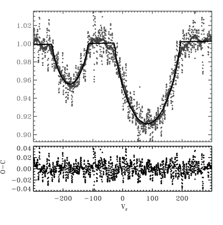
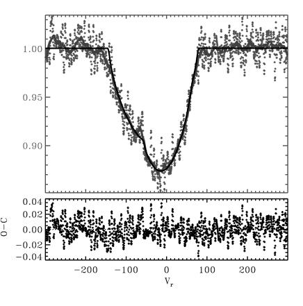
Figure 3: An example of the fit of the line profiles of Mg ii 4481 Å . The black solid line is the fit with a function obtained by summing the individual profiles of the components (a convolution of a gaussian and rotational broadening). For clarity a gray line is also shown, which corresponds to a smoothing with an averaging boxcar of width comparable to the FWHM of the interstellar Na ii D line (the narrowest lines appearing in the spectra). Left panel: unblended lines at phase $\varphi=0.71$, right panel: blended lines at $\varphi=0.45$. The lower boxes show the fit residuals.

Given that HD 174884 turned out to be a close binary, a spectroscopic campaign was organised as soon as possible after the CoRoT space photometry had become available to us. We used the CORALIE échelle spectrograph attached to the 1.2m Euler telescope at La Silla in Chile. The star was monitored from 7 to 16 June 2008, adopting an exposure time of 30 minutes. We used the online reduction package available for the CORALIE spectrograph and based on the method by Baranne et al. (1996). The process involves the usual steps of de-biasing, flat-fielding, background subtraction and wavelength calibration by means of measurements of a ThAr calibration lamp. All spectra were subsequently normalized to the continuum by fitting a cubic spline and barycentric corrections were computed for the times of mid-exposure. This led to barycentric wavelength-calibrated normalized spectra with a S/N ratio between 50 and 120 in the blue spectral region (the red parts suffered more from relatively poor atmospheric conditions during some nights). nspection of the spectra revealed that HD 174884 is a double-lined spectroscopic binary, evident line doubling could be seen in He i and, more clearly in Mg ii 4481 Å  line (see Fig. 3), identifying both components as stars of spectral type B. The finding of similar temperatures from the preliminary light curve solution was therefore fully confirmed.

The set of 45 spectra was independently analyzed with different methods: profile fitting of the abovementioned Mg ii line and Fourier spectra disentangling. The radial velocity curves from profile fitting were used in the simultaneous solution discussed in Section 3.1. Fourier disentangling provided the individual stellar spectra and allowed, as well, a cross-check with the results of radial velocity analysis, that turned out to be very useful, given the peculiarity of the system configuration.

Figure 4: The radial velocity curves for the two components of HD 174884 (dots: primary , triangles: secondary component). The phases are computed according to the ephemeris in Eq. 1, velocity unit is kms^-1. The solid line is the fit described in Section 3.1.

2.2.1 Radial velocity curves from profile fitting

We extracted the region 4450-4500 Å  and fitted the Mg ii 4481 Å line profile with a standard non-linear least squares fit procedure (IDL’s CURVEFIT) using a user-supplied non-linear function with an arbitrary number of parameters. The supplied function was a theoretical profile obtained by convolving for each star a Gaussian (corresponding to CORALIE spectra resolution) and a (dominant) rotationally broadened profile. In principle there were 8 adjustable parameters (position, width, depth of each profile and the values of continuum on the two sides). However, the iterative procedure did not converge in the case of heavily blended profiles. Therefore, we fitted first the unblended profiles, adjusting the full set of 8 parameters, and fixed then the rotational velocities, $v_{\mathrm{r}}\sin i$, to the average values obtained in this way for the remaining fits. These average values are $v_{\mathrm{r,1}}\sin i=109.3\pm 1.5$ kms^-1 and $v_{\mathrm{r,2}}\sin i=59.7\pm 2.7$ kms^-1.

The fits were performed on the original profiles and as well on the smoothed ones, with different boxcars (see Fig. 3 for examples). The results were very similar even with resolution degraded down to 0.025 Å/pix, i.e. the FWHM of the narrow NaI D interstellar lines (the narrowest lines seen in the spectra). The values in Table 2 correspond to the fit of the unsmoothed profiles. The fit uncertainties were derived with a bootstrap experiment (see Section 3.2), providing a more meaningful statistical estimate than formal errors of the fit.

Figure 5: A search for optimal values of $K_{1}$ and the mass ratio $K_{1}/K_{2}$.

Only 42 out of 45 spectra yielded a determination of radial velocities, for the remaining three, too close to conjunctions, the fitting procedure did not converge. The resulting values are collected in Table 2 and the radial velocity curves are shown in Fig. 4. The radial velocity curves were fitted with PHOEBE. This preliminary solution was not simultaneous, but we used an iterative procedure between light and radial velocity curve solutions, feeding the output of the iteration on one set of data as input to the other. The purpose was to get a set of input parameters for the final combined solution presented in Section 3. Actually the parameters obtained from the preliminary light curve fit of Section 2.1.1 were found to predict fairly well the radial velocity curves, apart of course from the mass ratio. The values best fitting the radial velocity curves alone were: $e=0.292\pm 0.003$, $\omega=51.85^{\circ}\pm 0.5$, $a\sin i=18.27\pm 0.08$ R_⊙, $\gamma=-20.7\pm 0.3$ kms^-1, $q=0.674\pm 0.005$ (formal errors). The corresponding radial velocity amplitude for the primary is $K_{1}=106.4\pm 0.6$ km s^-1.

2.2.2 Fourier disentangling of spectra

Southworth & Clausen (2007) carefully compared various possible present-day techniques to derive the orbital elements of spectroscopic binaries and concluded that the best results are obtained via properly applied disentangling. They showed that it is necessary to map the dependence of the sum of squares of residuals in the semiamplitudes $K_{1}$ and $K_{2}$ (or the mass ratio $K_{1}/K_{2}$) since this sum usually has a number of local minima in the parameter space.

To obtain reliable orbital elements of HD 174884 based on all 45 spectra we applied the disentangling in the Fourier domain developed by Hadrava (1995, 1997, 2004), using the latest publicly available version of his Fortran program KOREL, dated December 2, 2004.

In general, our experience with KOREL fully confirms the findings by Southworth & Clausen (2007) and also that the result is sensitive to the choice of starting values of the elements and initial values of the simplex steps, i.e. that the simplex solution can easily be trapped in a number of various local minima.

Table 3: KOREL disentangling orbital solutions for the three combined blue spectral regions near some stronger spectral lines useful for determination of atmospheric parameters, and for the red spectral region near the He I 5876 A line. The period, eccentricity and longitude of periastron were kept fixed at the values of 3$\aas@@fstack{d}$65705, 0.29394, and 51.$\!\!{}^{\circ}$31, respectively. The epoch of the periastron passage $T_{\rm periast.}$ is tabulated in HJD$-$2454628.

Element	3 blue regions	He i 5876
$T_{\rm periast.}$	0.69173	0.69037
$K_{1}$(km s-1)	106.983	106.956
$K_{2}$(km s-1)	159.39	161.64
$K_{1}/K_{2}$	0.6712	0.6617

The spectra at our disposal have a large resolution and it would be very time-consuming to carry out disentangling for the whole interval of wavelengths they cover. At the same time, the $S/N$ of the spectra is not particularly high. To cope at least partly with this problem and to obtain good disentangled spectra containing spectral lines sensitive to the determination of atmospheric paramaters and chemical abundances, we slightly degraded the spectral resolution, averaging the spectra over 0.05 A and used only the following four spectral regions: 4050 – 4190, 4450 – 4500, 4810 – 4910, and 5860 – 5885 A. For each spectral segment, we estimated the $S/N$ ratio of individual spectrograms and used the weights proportional to $(S/N)^{2}$. The disentangling was then carried out separately for the three blue spectral regions combined into one solution and for the red region near the He I 5786 A line where we also considered the telluric lines in the solution. In all cases, we derived also the relative line strengths for individual spectra during the solutions (Hadrava 1997). In all solutions, we kept the orbital period $P$, eccentricity $e$ and the longitude of periastron $\omega$ fixed at the values of 3$\aas@@fstack{d}$65705, 0.29394, and 51.$\!\!{}^{\circ}$31, respectively, which were derived from the final light curve fit (see next section). The epoch of the periastron passage $T_{\rm periast.}$ was chosen inside the time interval covered by the spectra, near HJD$-$2454628.7, but was allowed to converge.

Figure 6: Disentangled line profiles.

We first investigated the variation of the sum of squares of the residuals as a function of the radial velocity semi-amplitude of the primary only, keeping all other elements but the periastron passage fixed. This dependence was investigated separately for the combined blue, and the red spectral segment and is shown in a graphical form in the left panels of Fig. 5. This led to the conclusion that the true semi-amplitude of the primary must be close to 107 km s^-1. Fixing this value of the semi-amplitude, we then investigated the sum of squares of residuals as a function of the mass ratio, again separately for the blue and red spectral segments. This also rather uniquely restricts the plausible values of the mass ratio to 0.66-0.67 (cf. the right panels of Fig. 5).

The final disentangling was then derived starting with the best values found and allowing for the convergence of $K_{1}$, $K_{1}/K_{2}$, and $T_{\rm periast.}$. We did a number of trial solutions for each spectral segment, varying slightly the initial values of the elements and starting simplex steps to find out solutions with the smallest sums of residuals. The results are summarized in Table 3. Their comparison provides some idea about the probable errors of the elements. We remind that for the region $5860-5885$ A, we also included the weak telluric lines into the solution. The comparison of results is useful since the program KOREL we used does not provide any estimate of the errors of the elements.

We included KOREL results in PHOEBE as cross-check, following a somewhat unusual procedure. For each of the four KOREL solutions we extracted radial velocities of both components for the 45 times of observations and derived their average values over the two solutions for each BJD, giving 3 times higher weights to the blue RVs based on the separate spectral segments. These “mean theoretical” RVs were used to verify the results from PHOEBE that are based on profile fitting RV curves; we find excellent agreement between the two methods of RV extraction.

Keeping the elements from the final PHOEBE solution, discussed in the next section, fixed, we disentangled the binary spectra. They are shown in Fig. 6.

3 Final analysis

3.1 Simultaneous light and radial velocity curve fit

To obtain a set of parameters that most accurately describes physical and geometric properties of HD 174884, we submitted photometric and RV data in the time domain to a simultaneous fitting process in PHOEBE. Simultaneous fitting imposes consistency of the solution across all available data-sets.

The initial values of $T_{\mathrm{eff},1}$ and $T_{\mathrm{eff},2}$ were adopted from the previous preliminary fits: $13,140$ K and $11,000$ K, respectively. The values of gravity darkening coefficients and albedoes were set to their theoretically expected values for radiative envelopes: $g_{1,2}=1.0$; $A_{1,2}=1.0$. The center-of-mass radial velocity $v_{\gamma}$ was derived from the RV fit and held constant.

We used the RV derived value of $a\sin i=18.27\pm 0.08$ R_⊙(cf. §2.2.1) to constrain the solution to those values of $a$ and $i$ that preserve $a\sin i$. Line profile analysis and spectrum disentangling (cf. §2.2.2) yield consistent values of $v_{1}\sin i=109.3\pm 1.5\,\mathrm{km\,s}^{-1}$ and $v_{2}\sin i=59.7\pm 2.3\,\mathrm{km\,s}^{-1}$; these were used to constrain synchronicity parameters $F_{1,2}=\omegaup_{\mathrm{rot}}/\omegaup_{\mathrm{orb}}$, i.e. the ratio of rotation to mean orbital angular velocity. Square-root limb darkening coefficients are interpolated on-the-fly from PHOEBE lookup tables, based on the current values of $T_{\mathrm{eff}}$, $\log g$, $[M/H]$ and $v_{\mathrm{rot}}$ for each star. As before, passband luminosity was computed rather than adjusted, to enhance convergence. The constraints are imposed during each iteration, projecting out only those solutions that satisfy the embedded physical requirements.

Parameters that were adjusted are: eccentricity $e$ and argument of periastron $\omega$, inclination $i$, surface potentials $\Omega_{1}$ and $\Omega_{2}$, mass ratio $q$, and secondary surface temperature $T_{\mathrm{eff},2}$. The mass ratio typically has little detectable signature in well detached EB light curves since it affects ellipsoidal variations; in the case of HD 174884, however, the CoRoT light curve’s sensitivity on $q$ is significant, due to the eccentric orbit, the consequent star shape distortion and high data accuracy. These factors allowed us to adjust the value of $q$ based on simultaneous LC and RV data. There is an excellent agreement between the $q$ value from the final fit and that derived from KOREL. The difference is less than 1-sigma interval for the three blue segments and within 2 sigma for the red one (which has a lower S/N ratio).

The final parameter set is listed in Table 4.

Table 4: Physical and geometric parameters of HD 174884.

Parameter:		System
	Primary		Secondary
$a$ (R⊙)		$18.88\pm 0.14$
$i$ (∘)		$75.35\pm 0.03$
$q=\mathscr{M}_{2}/\mathscr{M}_{1}$		$0.674\pm 0.009$
$e$		$0.2939\pm 0.0005$
$\omega$		$51.31^{o}\pm 0.06^{o}$
$v_{\gamma}$ (km s-1)		$-20.6\pm 0.3$
$\Omega$	$6.055\pm 0.008$		$7.866\pm 0.020$
$T_{\mathrm{eff}}$ (K)	13140		$12044\pm 50$
$\mathscr{M}$ (M⊙)	$4.04\pm 0.11$		$2.72\pm 0.11$
$\mathscr{R}$ (R⊙)	$3.77\pm 0.03$		$2.04\pm 0.02$
$M_{\mathrm{bol}}$	$-1.71\pm 0.04$		$0.01\pm 0.05$
$F=\omegaup_{\mathrm{rot}}/\omegaup_{\mathrm{orb}}$	$2.0^{*}\pm 0.2^{*}$		$2.3^{*}\pm 0.2^{*}$
∗computed from the observed $v\sin i$ and orbital period.

Before adopting our final solution and proceding to comparison with the stellar models we felt there were still two questions to address: solution uniqueness and a realistic estimate of the uncertainties.

It is well known that light curve solutions can be affected by uniqueness problems, and this could be a serious issue in the case of our light-curve that features a grazing eclipse. It is also well known that the formal errors derived from least squares covariance matrix are inaccurate because the parameter space axes are not orthogonal and marginalization around the solution is not fully justified. More realistic errors were derived by bootstrap and by full-fledged heuristic scanning, performed on all adjusted parameters. The latter procedure provides information on the morphology of the cost function hyper-surface in the adjusted parameter space.

Figure 7: The contour enclosing 68.3% of all bootstrap solutions (1-sigma uncertainties) for two pairs of parameters: upper panel $i$ – $\Omega_{1}$, lower panel $\Omega_{1}$ – $T_{{\rm eff,2}}$. The solid cross is the median of bootstrap solution values; the arm length is equal to the uncertainty on the single parameters, not taking correlation into account (i.e the interval of the parameter containing 68.3 % of solutions). The broken-line cross is our final solution with arms equal to the standard errors. The small offset is due to the fact that bootstrap solutions, because of repetitions, are obtained from a curve with a different (and worse) sampling than the original light-curve. The projections of the contours on the axes provide the uncertainties of (correlated) parameters mentioned in the text.

The final estimates of most parameter uncertainties appearing in Table 4, is obtained by the heuristic scan presented in Section 3.3. As, however, this is a procedure rather expensive in terms of computing time and resources , we found it instructive to compare the results of both methods, and quantify the differences. Furthermore, we adopted the uncertainties from bootstrap for the parameters not adjusted in the scan.

3.2 Parameter uncertainties by bootstrap

Bootstrap resampling is a very useful technique to estimate parameter confidence levels of least squares solutions (see, for instance Press et al. 1992). The method consists in generating many different data samples by random resampling with repetitions (bootstrapping) the available data, performing the minimization procedure for each sample and deriving confidence intervals from the resulting distribution of parameters. The advantage, with respect to the errors derived from least squares solutions, is that a plot of the parameter distributions directly shows the effect of inter-parametric correlations, and that the confidence intervals are not linked to Gaussian distributions of the residuals. In the parameter space the one-sigma confidence levels, for instance of a pair of correlated parameters, is defined as the projection on the parameter axes of the contour containing 68.3 % of the bootstrap solutions.

In this paper we used bootstrap resampling to estimate the errors on radial velocities, as obtained from profile fit. This is a standard application of the technique: the fitting procedure is repeated (1000 times), after bootstrapping the fit residuals. In principle the same technique can be used also to estimate the uncertainties of the light and radial velocity curve fit, with the advantage of deriving more realistic errors than that the formal ones and of gaining insight on parameter correlations. It is not straightforward, however, to apply the bootstrap technique to the complex light curve solution process, because a complete minimization process should be performed for thousands of bootstrap data-sets. A simpler approach was suggested by Maceroni & Rucinski (1997) who applied bootstrap resampling within the minimum already established by a single iterated solution (that is, using only one set of residuals and parameter derivatives). This approach, as discussed in detail in the abovementioned paper, provides underestimated uncertainties with respect to a full bootstrap procedure, as it is applied already in a minimum, but nevertheless, the confidence level we estimated for the parameters are always larger than the errors from least square minimizations and have a clear statistical meaning.

The bootstrap uncertainty intervals were, therefore, obtained repeating, in this case, 10000 times the last iteration of the fit, after random permutation of the residuals. Fig. 7 shows two 2-D projections of the n-dimensional distribution of the resulting parameter sets ($i$ – $\Omega_{1}$ and $\Omega_{1}$ – $T_{{\rm eff,2}}$). The figure allows a direct comparison between the standard deviations from the PHOEBE last iteration and two confidence intervals derived from bootstrap: that of each single parameter, not taking correlation into account, i.e. its interval containing 68.3% of solutions, and the 1-sigma confidence level of parameter pairs (the contours), clearly showing the effect of correlations (see the plot for the pair $\Omega_{1}$ – $T_{{\rm eff,2}}$). The projection of the contours on the axes provides a measure of the uncertainty taking parameter correlations into account.

The error estimates obtained by this simplified bootstrap procedure are somewhat smaller but still the same order than those from the heuristic scanning of next section. Taking the largest of the full width 1-sigma intervals (as bootstrap errors are not symmetric) among various projections and comparing with the uncertainties of the heuristic scan of Table 4 we have, 0.02 vs 0.06 for $i$ (bootstrap vs heuristic scan), 0.01 vs. 0.016 for $\Omega_{1}$, 0.01 vs. 0.04 for $\Omega_{2}$ and, 40 vs 100 for $T_{{\rm eff,2}}$. The formal errors of the fit are typically several times smaller.

The upper panel of Fig. 7 suggests as well a complex shape of the cost function along inclination, as the 1-sigma contour corresponds to a bimodal distribution of the solutions. That feature is fully revealed by the heuristic scan.

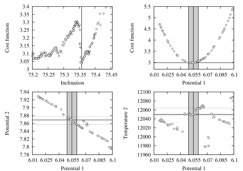
Figure 8: The results of heuristic scanning. Top two panels depict the projection of the cost function space along inclination (left) and primary surface potential (right). The bottom two panels depict correlations between the secondary surface potential (left) and secondary effective temperature (right). A gray stripe encompasses 1% deviations from the minimum cost function value in the primary surface potential, obtained by fitting a parabola to the top right panel. Solid lines represent the best-fit solution, while dashed lines represent parameter limits as determined by the plausible primary surface potential values.

3.3 Heuristic scanning of parameter space

Heuristic scanning (Prša & Zwitter 2005) is a Monte-Carlo based method to map parameter correlations and cost function degeneracy. Scanning produces an $N$-dimensional cost function map, where $N$ is the number of adjusted parameters. Projections in that $N$-dimensional parameter space reveal solution degeneracy.

We performed the scanning in two sequential steps: the first one along inclination, fitting $\Omega_{1}$, $\Omega_{2}$, $T_{\mathrm{eff}},2$ and computing $L_{1}$, $x_{LD}$ and $y_{LD}$, and the second one along the primary surface potential, fitting and computing the same parameters except for the inclination.

Because of the unprecedented accuracy of CoRoT light curve, a typical $\Omega_{1}$ degeneracy with inclination, surface potential $\Omega_{2}$ and effective temperature $T_{\mathrm{eff},2}$ is essentially broken. There is a clear $\chi^{2}$ minimum both in inclination (Fig. 8, top left panel) and primary surface potential (top right panel) that narrowly constrain the uniqueness of the solution. It was very instructive to observe the behavior of inclination with the mass ratio: the cost function profile varies quite substantially with the changing value of $q$. Although the location of the global minimum remains unaffected, adjacent local minima gain on depth, predominantly at the expense of “sacrificing” the fit to the secondary minimum to better match the abundant out-of-eclipse regions. This indicates that the model we are using to fit the data is pushed to its limit and systematic errors begin to have a significant impact on the overall error budget of the solution.

4 Physical properties of HD 174884

4.1 Comparison with evolutionary models

The comparison between the physical parameters obtained for HD 174884 components and the stellar models was done according to the method described in Miglio & Montalbán (2005) and Miglio et al. (2007). That consists in applying a Levenberg-Marquardt gradient descent algorithm (Bevington & Robinson 2003) to minimize a quality function which describes the discrepancy between the models and the observables:

$$\chi^{2}=\sum_{i=0}^{No}\,\frac{(O_{i}^{obs}-O_{i}^{theo})^{2}}{(\sigma_{i}^{obs})^{2}}.$$ (2)

The procedure iteratively adjusts free parameters of the models, yielding $O_{i}^{theo}$, until best fit is reached. In our case the “observables” ($O_{i}^{obs}$) are the system parameters derived in the previous sections: $\mathscr{M}_{1}$, $\mathscr{R}_{1}$, $T_{\rm eff,1}$, the effective temperature difference between components, ($\Delta T_{\rm eff}$), the mass ratio ($q$), the radius ratio ($k$) and metallicity. The corresponding errors are $\sigma_{i}^{obs}$. Though we initially chose as observables the absolute values (masses, radii, temperatures), we finally preferred to use the parameters of the primary component and their ratios or differences with respect to the secondary, since the light curve solution is mainly sensitive to relative values. For the uncertainty on $\Delta T_{\rm eff}$ we assumed, on the basis of the light curve fit results, a value of of 100 K. As the available data were not accurate enough to derive metallicity, we assumed different values of $[{\rm M}/{\rm H}]$ with an uncertainty of 99%.

Table 5: Best fit models. The values of the “observables” , $O_{i}^{obs}$, are given for comparison in the note.

Model	$\mathscr{M}_{1}$	$\mathscr{M}_{2}$	$Z$	$X$	Age	$OV_{2}$	$\mathscr{R}_{1}$	$\mathscr{R}_{2}$	$T_{\rm eff\,1}$	$q$	$k$	$\Delta T_{\rm eff}$
	(M⊙)	(M⊙)			(Myr)		(R⊙)	(R⊙)	(K)			(K)
A	4.05$\pm$0.09	2.74$\pm$0.06	0.014$\pm$0.003	0.728$\pm$0.090	121$\pm$49	0.000	3.76	2.03	13189	0.676	0.541	1631
AC	4.04$\pm$0.11	2.75$\pm$0.08	0.011$\pm$0.003	0.720∗	112$\pm$9	0.062	3.68	1.97	13737	0.682	0.537	1520
B1	3.99$\pm$0.08	2.74$\pm$0.06	0.011$\pm$0.002	0.740∗	131$\pm$9	0.000	3.77	2.00	13097	0.688	0.530	1310
B2	4.02$\pm$0.08	2.77$\pm$0.06	0.010$\pm$0.002	0.720∗	115$\pm$8	0.000	3.77	2.00	13614	0.689	0.530	1338
C6	4.01$\pm$0.08	2.76$\pm$0.06	0.012$\pm$0.002	0.720∗	118$\pm$ 9	0.200	3.77	2.00	13339	0.688	0.530	1295
C1	4.05$\pm$0.11	2.78$\pm$0.08	0.018$\pm$0.010	0.738$\pm$10.2	131$\pm$57	0.654	3.77	2.02	12668	0.685	0.536	1305
C4	4.04$\pm$0.11	2.77$\pm$0.08	0.015$\pm$0.007	0.740∗	130$\pm$13	0.355	3.77	2.02	12870	0.686	0.535	1320
C2	4.00$\pm$0.08	2.75$\pm$0.06	0.013$\pm$0.002	0.740∗	131$\pm$10	0.200	3.77	2.00	12978	0.687	0.530	1277
C5	4.00$\pm$0.08	2.75$\pm$0.06	0.012$\pm$0.002	0.740∗	131$\pm$1	0.100	3.77	2.00	13045	0.688	0.530	1293
C7	3.99$\pm$0.08	2.75$\pm$0.06	0.011$\pm$0.002	0.740∗	130$\pm$95	0.050	3.77	2.00	13078	0.688	0.530	1298

• $O_{i}^{obs}$: $\mathscr{M}_{1}=4.04\pm 0.11$; $\mathscr{R}_{1}=3.77\pm 0.03$; $T_{\rm eff\,1}=13140\pm 1500$; $q=0.674\pm 0.009$; $k=0.541\pm 0.013$; $\Delta T_{\rm eff}=1096\pm 100$ (or 1240$\pm 100$, see text).

• For all models $OV_{1}=0$. Model AC belongs both to group A and C. Several C-type models are listed to illustrate the effect of adjusting $OV_{2}$.

• ^∗) Fixed value.

The theoretical values ($O_{i}^{theo}$) are obtained from stellar evolution modeling with the code CLES (Code Liégeois d’Évolution Stellaire, Scuflaire et al. 2008b). In all model computations we used the mixing-length theory (MLT) of convection (Böhm-Vitense 1958) and the most recent equation of state from OPAL (OPAL05, Rogers & Nayfonov 2002). Opacity tables are those from OPAL (Iglesias & Rogers 1996) for two different solar mixtures, the standard one from Grevesse & Noels (1993, GN93) and the recently revised solar mixture from Asplund et al. (2005, AGS05) . In the former $(Z/X)_{\odot}$=0.0245, in the latter $(Z/X)_{\odot}$=0.0167. These tables are extended at low temperatures with Ferguson et al. (2005) opacity values for the corresponding metal mixtures. The surface boundary conditions are given by Kurucz (1998) atmosphere models.

The parameters of the stellar model are: mass, initial hydrogen ($X_{\rm i}$) and metal ($Z_{\rm i}$) mass fractions, age and two convection parameters ($\alpha_{\rm MLT}$ and the overshooting parameter $OV$). All of them, or just a subset, can be adjusted in the minimization. The value of $\alpha_{\rm MLT}$ was kept fixed, adopting the solar value of 1.8, as it has no relevant effect on the evolutionary tracks of models with masses in the domain of interest here.

Different minimizations were done with $X_{\rm i}$ as a free parameter or fixed to different values between 0.69 and 0.74. Similarly, the overshooting parameter, which describes the size of the extra-mixed region close to the convective core, was kept fixed at values between 0.0 and 0.4, but in some cases left free. Binarity puts an additional constraint on chemical composition and age, which can be assumed to be the same for the components. Therefore, the number of free parameters varied from four ($\mathscr{M}_{1},\,\mathscr{M}_{2},\,Z,\,$ age) to six : $\mathscr{M}_{1},\,\mathscr{M}_{2},\,X,\,Z,\,OV\,$ and age. We performed two sets of minimizations, the first with the same physical description of components (essentially same value of overshooting parameter), and the second allowing a different parametrization of extra-mixing.

Regardless of these physical details all computations show the same trend: if the $\Delta T_{\rm eff}$ is well fitted (within 1-$\sigma$) the mass ratio is larger than the observationally derived value and the deviation is typically between 2 and 3$\sigma$ . This fact can be explained considering that for two stars with the same initial chemical composition and physical processes, fixing the effective temperature difference at given age is essentially equivalent to fixing the mass difference. Due to correlation, any combination of $\Delta T$ and $q$ yields estimates on $q$ that are inconsistent with the light and radial velocity curve solution. This behavior is evident in Fig. 9 which shows the iso-$\chi^{2}$ contours in the q–$\Delta T_{\rm eff}$ plane. This plot was built using the several thousands binary models computed in the minimization processes. If the constraint on $\Delta T_{\rm eff}$ is relaxed, the fit within 1$\sigma$ for all the other constraints is achieved, but $\Delta T_{\rm eff}$ is $\sim\,1600$ K (Model A of Table 5). Among the minimizations performed with same physics, $\Delta T_{\rm eff}=1310$ K is the minimum difference of effective temperature that we were able to achieve, keeping the mass and radius ratios within 2$\leavevmode\nobreak\ \sigma$ (1.6$\sigma$ for $q$ and 1.3 $\sigma$ for $k$) (Model B1). These best fits were obtained from computations without overshooting. Values of $OV$ larger than zero generally lead to smaller primary masses and hence larger $q$ values.

Is it possible to reconcile the observed values of $q$ and $\Delta T_{\rm eff}$ with those from the theoretical models? To answer this question we considered the possible alternatives and the weak points of comparison with the models. An evident inconsistency between the stars and the corresponding models is that CLES computes spherical non-rotating models, while the primary and secondary component of HD174884 rotate, respectively, at 25% and 12% of their break-up critical velocity, and are significantly non-spherical. The distortion of the primary ($R_{pole}$ $\sim\,2.5$% smaller than $R_{\rm eq}$) is mainly due to rotation. It is well known that at given mass, rotating stars appear to be cooler than non rotating ones, or – expressed in different terms – at given effective temperature, non-rotating models will assign lower stellar masses than rotating ones. The difference of effective temperature between rotating and non-rotating models depends on the rotational velocity, inclination of the rotation axis and chemical composition of the star (see, e.g., Maeder & Meynet 2004). An estimate of the average effect of rotation on the observed effective temperature for moderate rotators is provided by Bastian & de Mink (2009) and their results are in agreement with those of the Geneva group for a 4 M_⊙ star (Meynet, private communication). According to the above-mentioned authors, the change in $T_{\rm eff}$ of a rotating star with respect to a non-rotating one can be expressed as :

$$T_{\rm eff}(\eta)/T_{\rm eff}(0)=1-a\eta^{2},$$ (3)

where $\eta$ is the fraction of the critical break-up rotation rate, $T_{\rm eff}(0)$ is the effective temperature of the non-rotating model, and $a$ is a coefficient which changes from 0.17 at zero age to 0.19 at the end of the main sequence. In the case of HD174884, the apparent decrease in temperature due to rotation amounts to $\sim 160$ K for the primary and only 20 K for the secondary component. As consequence, the observed effective temperature difference should be smaller than that of non-rotating models, and that could explain the higher $\Delta T_{\rm eff}$ values from best fit models with respect to that from the light curve solution. In this hypothesis, the constraint on $\Delta T_{\rm eff}$ to be used with our non-rotating models shall be increased from 1096 K to $\sim\,1240$ K. This value, however, is still somewhat lower than that obtained in our best fit.

The value of the overshooting parameter, its dependence on the stellar mass, and the physical origin of the extra-mixing are still a matter of debate. A different value for the two components cannot be completely excluded and the hypothesis $OV_{1}=OV_{2}$ could be dropped. We tried, therefore, to satisfy our observational constraints by using fixed and different values of $OV_{1}$ and $OV_{2}$. We also performed computations fixing $OV$ for the primary and varying the $OV$ for the secondary component, and - as well - keeping fixed $OV_{2}$ and deriving $OV_{1}$. The corresponding models are labeled as models C in Table 5. An overshooting parameter higher for the secondary than for the primary slightly improves the fit with respect to model B. From a physical point of view, we could justify a secondary with a stronger mixing in the center, even if its rotational velocity is lower than that of the companion, by invoking an important gradient of the internal rotational profile produced by braking in the synchronization process. However, the improvement in the fit is not significant enough to justify the introduction of an additional parameter.

The age of the system is similar for all models and has an average value of $125\pm 7$ Myr.

Finally, we can ask ourselves if our conclusions could depend on the evolutionary code we used for computing stellar models. A convincing answer to this question can be found in the extensive study which was carried out by the CoRoT/ESTA (Evolution and Seismic Tools Activity) group, in view of the CoRoT mission and the foreseen analysis of seismic data of the highest ever achieved accuracy. The team made an accurate comparison among different evolutionary and pulsation codes for selected test cases. Their results (Lebreton et al. 2008, and other contributions appearing in the same special issue) allow us to conclude that in the part of the parameter space of interest here (MS stars of intermediate mass) stellar evolutionary codes adopting the same physics yield the same fundamental parameters and the same internal structure.

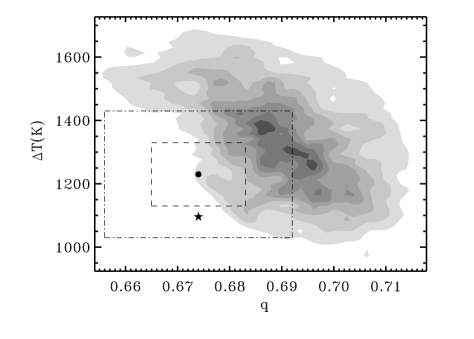
Figure 9: The iso-$\chi^{2}$ contours in the q–$\Delta T_{\rm eff}$ plane for the Levenberg-Marquard minimizations of the deviations with respect to theoretical models. Lower values correspond to darker colors. The plot clearly shows the correlation between the two parameters. The $\chi^{2}$ is computed with respect to the $\Delta T_{\rm obs}$ value obtained after correction for the effect of rotation (see text). The original value is also shown, as a starred dot. The broken line boxes enclose 1- and 2-$\sigma$ intervals.

4.2 Orbital evolution

The position of HD 174884 in the period-eccentricity diagram of close binaries is shown in Fig. 10. The plot is based on the catalog of Hegedüs et al. (2005), with the addition of HD 313926, a short period (P=2$\aas@@fstack{d}$27) high eccentricity (e=0.21) eclipsing binary formed by two B-type stars, which was recently discovered by the MOST satellite (Rucinski et al. 2007). The majority of B-binaries in the figure have main sequence components. HD 174884 has the second highest eccentricity among binaries with B type components.

Figure 10: The period - eccentricity diagram, for close binaries according to the catalog of Hegedüs et al. (2005). Filled circles correspond to B stars, open circles to A-G stars. The star symbol indicates the location of HD 174884, the triangle that of HD 313926 (Rucinski et al. 2007, see text).

Rucinski et al. (2007) suggest that the upper envelope for B type stars in the period-eccentricity plot might be flatter than that of the later stellar types. This can be understood in terms of stronger dissipation, and hence more efficient circularization mechanisms, for stars with larger fractional radii, see for instance the review of Zahn (2005). That is at the origin of the overall trend in the plot (lower eccentricity for shorter periods), besides, at fixed period, less massive (unevolved) stars have smaller fractional radius and hence longer circularization timescales. The evidence of the second effect is, however, marginal in our updated plot, as HD 174884 occupies a region previously empty of B-stars.

The relation between eccentricity and the fractional radius of early type binaries has been extensively studied. Giuricin et al. (1984) analysed a sample of galactic binary and North & Zahn (2003) more homogeneous ones in the Magellanic Clouds. All samples indicate the existence of a “cut-off” fractional radius, above which all systems have circular orbits. This value – practically independent of chemical composition – is $\simeq 0.25$. The fractional radius of HD 174884’s primary is $r_{1}\simeq 0.2$, i.e. a value consistent with its elliptic orbit. Its position in the eccentricity vs. fractional radius plot of Giuricin et al. (1984) (not shown here for the sake of brevity) marks again the upper envelope of the galactic sample for that period.

The same mechanism producing orbit circularization is at the origin of spin-orbit synchronization on timescales typically a few orders of magnitude shorter than that for circularization, as – in presence of efficient angular momentum transfer – the ratio of the two timescales equals that of rotational and orbital angular momentum content. As long as the orbit is elliptical, the component rotation will synchronize with the orbital motion at periastron. Since $v\sin i$ was estimated from spectral analysis ($v_{1}\sin i=109\mathrm{km\,s}^{-1},v_{2}\sin i=60\mathrm{km\,s}^{-1}$) and the eccentricity is well constrained from spectrophotometric modeling, we can readily verify whether this is the case. A theoretical value (Hut 1981) of the synchronicity parameter for synchronous rotation at periastron is $F=\sqrt{(1+e)/(1-e)^{3}}$, and for our system $F=1.92$, while spectroscopic analysis yields $F_{1}=2.0\pm 0.2$ and $F_{2}=2.3\pm 0.2$. Both stars thus seem to be rotating marginally super-synchronously. We can check if the dynamical state of the system is in agreement with the expected timescales. If we follow Zahn’s formalism (see the above-mentioned review and Claret & Cunha 1997) to estimate the circularization and synchronization timescales of HD 174884, adopting a value of $\beta=0.2$ for the fractional gyration radius (Claret & Gimenez 2005) and $\log E_{2}=-6.6$ for the value of the second torque constant (Claret & Cunha 1997), we get: $\tau_{\rm circ}=8.9\cdot 10^{8}$ yr ( or 35% shorter considering the contribution of both components), $\tau_{\rm sync,1}\simeq\tau_{\rm circ}/120=7.4\cdot 10^{6}$ yr and $\tau_{\rm sync,2}\simeq 4\tau_{\rm sync,1}$. While the relations providing these estimates are derived under the hypothesis of small deviation from circular orbit and synchronism, the resulting figures are indeed in good agreement with the dynamical status of our system.

The fact that in the same period interval of the $e$–$P$ plot both circularized and elliptic orbits can be found is interpreted (Zahn 2005) as due to much higher efficiency of tidal damping when resonance locking (Witte & Savonije 1999) takes place. As this event is very sensitive to the binary parameters it might appear only in some systems among those of similar period, depending on the other stellar parameters. According to this interpretation the orbital evolution of HD 174884 has not been driven by resonance locking.

4.3 Pulsational properties: analysis of light-curve fit residuals

The residuals from the phased light curve fit, appearing in the lower panel of Fig. 2, clearly show a phase-locked pattern, which can be described in terms of two components: a complex irregular structure at phases close to (and within) primary eclipse and a multi-periodic oscillatory behaviour at other phases. Their different nature is suggested by the fact that only the latter is present in the original light curve (see Fig. 11).

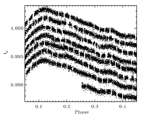
Figure 11: Sections of the original light curve, phased according to the orbital period and vertically shifted for better clarity. The seven observed orbital periods go bottom-up. The oscillatory pattern of the residuals is clearly seen in each curve.

We interpret the first component as due to systematic effects caused by the employed EB model, e.g. to small deviations in model atmospheres (and consequently in the limb darkening description), and to the description of stellar surfaces by a finite, though large, number of elements. These effects are expected to be visible during eclipses, when one stellar disc eclipses the other. Those related to the surface discretization are typically below 0.1 mmag, but can be larger at some critical phases.

Table 6: Results of Fourier analysis

F$n$	Frequency	Amplitude	Phase	S/N	Remark
	(d-1)	($10^{-3})$
F1	0.273444	0.452 $\pm 0.002$	0.3848 $\pm 0.0006$		$f_{\rm orb}$, fixed
F2	0.5470 $\pm 0.0002$	0.284 $\pm 0.002$	0.840 $\pm 0.001$	14.2	$\simeq 2f_{\rm orb}$
F3	2.1858 $\pm 0.0004$	0.120 $\pm 0.002$	0.349 $\pm 0.002$	12.0	$\simeq 8f_{\rm orb}$
F4	3.5534 $\pm 0.0004$	0.111 $\pm 0.002$	0.822 $\pm 0.003$	11.2	$\simeq 13f_{\rm orb}$
F5	1.0894 $\pm 0.0004$	0.097 $\pm 0.002$	0.840 $\pm 0.003$	6.2	$\simeq 4f_{\rm orb}$
F6	0.0631 $\pm 0.0004$	0.116 $\pm 0.002$	0.931 $\pm 0.003$	7.2	long term trend
F7	0.8206 $\pm 0.0005$	0.091 $\pm 0.002$	0.570 $\pm 0.003$	7.8	$\simeq 3f_{\rm orb}$

We attempted to identify those segments of the code that need to be restated in order to increase the model accuracy. An important one is the above-mentioned surface discretization, which currently relies on equidistant partitioning of the surface along stellar latitude and longitude. This introduces a ”seam” along $\varphi=0$ where all surface elements are perfectly aligned. We have been devising a modified approach where surface elements are determined by equidistant partitioning along the length of the equipotential and shifted by half the element width at $\varphi=0$. Preliminary tests indicate that the systematic discrepancy in the vicinity of the primary minimum residuals (around $\varphi=-0.025$) is greatly reduced when employing the new strategy. However, significant testing is required to identify any potential problems with the new scheme.

The second component of the residuals, the oscillatory pattern which can be spotted by eye in the original curve, is certainly model-independent and is due either to the intrinsic variability or to an instrumental artifact. The latter hypothesis is, however, unlikely, given the perfect phasing with the binary period over more than seven cycles. Furthermore, none of the known frequencies of instrumental origin is close to those found in the pattern components.

Figure 12: The Fourier spectrum of the “cleaned” residuals after pre-withening of the first two frequencies in Table 6. The dotted lines mark the two frequencies 8 $f_{\rm orb}$ and 13 $f_{\rm orb}$. The dashed line is the spectrum of noise, computed by Period04 on the residuals. The inset shows the spectral window.

To extract the individual frequencies we performed a Fourier analysis with Period04 (Lenz & Breger 2005). For this purpose a complete set of residuals, in the time domain, was obtained by subtracting the fitted model from the $\sim$ 60000 points of the original light curve. The analysis is made more complex by the presence in the time series of residuals produced by the above-mentioned systematic effects, which generate power at the orbital frequency ($f_{\rm orb}=0.273444$ d^-1) and its overtones. The analysis was therefore performed on two different time strings: the complete set of residuals and a “cleaned” sub-sample, obtained by deleting the points the phase interval $-0.1\leq\varphi\leq 0.05$. Given the high total number of points it was possible as well to analyze only some sections of the light curve residuals, e.g. each individual period.

All the analyses provide essentially the same result: a clear detection of two frequencies, corresponding to 8 and 13 times the orbital frequency and marginal detections of other orbital overtones. Table 6 and Fig 12 summarize the results of the analysis for the “cleaned” set of residuals. The first frequency corresponds to $f_{\rm orb}$ and was kept fixed. The first two frequencies are actually needed to fit the slow trend, visible in the lower panel of Fig. 2, due to the systematics introduced by subtraction of the light curve model. Similarly the low frequency F6 fits a long term residual trend, a left-over of the detrending procedure which was applied to the original curve. Frequencies F3 and F4 correspond to $8f_{\rm orb}$ and $13f_{\rm orb}$.

The detections are very clear, reaching amplitudes over ten times the noise level. More multiples of the orbital frequency are present, but at lower amplitude so we consider them to be only marginal detections. Intrinsic variability at multiples of the orbital frequency are a phenomenon pointing towards tidally induced oscillations or free oscillations affected by the close binarity.

Even though several pulsating stars in close binaries have been found (e.g. Aerts & Harmanec 2004), oscillation frequencies at multiples of the orbital frequency have only seldomly been detected. The most likely explanation is that they are due to resonant dynamic tides which can lead to detectable amplitudes. As discussed by, e.g., Willems & Aerts (2002), the shape of tidally induced observables (light curves or radial velocities) can vary from very irregular for orbital periods away from a resonances with free oscillation modes to sinusoidal for orbital periods close to a resonance with a free oscillation mode. It is somewhat surprising that we find clear multiples of orders 13 and 8 for HD 174884, while the lower order multiples are not so markedly found. Interestingly, such a case also occurs for the slowly pulsating B star HD 177863, where an oscillation frequency of exactly ten times the orbital frequency was found and interpreted as due to resonant excitation (De Cat et al. 2000).

According to theory, tides can efficiently excite the free oscillation modes of the star which are close to the tidal frequency (and its multiples in eccentric orbits see, e.g., Willems 2003). The dominant tidal term is associated with the spherical harmonics of degree $\ell=2$. Besides, given the typical values of the tidal frequencies in close systems, the stellar free oscillation modes should be g-modes, and typically of high radial order, $n\gtrsim 10$ (Zahn 2005).

By means of the code LOSC (Liège OScillation Code Scuflaire et al. 2008a) we computed the eigenfrequencies of the primary star for all the models within 2-$\sigma$ in mass and radius and $\Delta T_{\rm eff}\lesssim 1600$ K. The purpose was to check the properties of the $\ell=2$ modes close to the F values of Table 6. LOSC includes the effects of rotation on the frequencies in a perturbative approximation, and the correction terms are limited to the first order in $\omega_{\rm rot}$ (e.g. Ledoux 1951). This approach is acceptable when the effects of the centrifugal force and of Coriolis acceleration are small. The former is estimated by the ratio ($\epsilon$) between the rotational period and the dynamical time , the latter by the ratio ($\mu$) of rotation to oscillation frequencies. For the HD 174884 primary component $\epsilon\sim 4\times 10^{-2}$ and $\mu=0.25$ for $F3$, and $\mu=0.15$ for $F4$. As shown by Miglio et al. (2008), the effect of rotation on the internal chemical composition profiles can also lead to slight changes of the eigenfrequencies.

Since our aim is not to fit the observed frequencies, but to verify that their value is well in the range of $\ell=2$ g-modes with radial order $n$ of $\sim$10 or larger, we consider the first order approach sufficient. The comparison between observed and theoretical frequencies indicates, indeed, that the lower frequency $F3$ corresponds, for the models described in Table 5, to $n$ values between 8 and 10, and the higher one to slightly larger values. We can conclude, therefore, that the frequencies we find in the residuals are compatible with tidally forced oscillations.

As a further check of the light curve solution robustness, we pre-withened the original curve by the two frequencies F3 and F4 and recomputed the best fit. The new solution is essentially the same as the old one: the largest difference between best-fit parameters before and after pre-withening is $0.4$%. The subtraction of the harmonic pattern does not substantially improve the correlation of residuals, because their dominant component, which we interpreted as due to model systematics, is essentially left unchanged by the procedure.

5 Summary and conclusions

This work has been carried out with two aims in mind: to achieve a thorough description of an interesting binary and to test the performance of current binary star modeling on data of unprecedented accuracy, as those available for the CoRoT seismo-field targets. HD 174884 lends itself to both purposes: its peculiar light curve suggests an unusual system configuration, worth a detailed study, and it is as well quite stable over the seven observed orbital periods so that, if possible systematic errors arising from binary modeling were present, they would not be hidden by transient intrinsic phenomena. (The latter is indeed the case of the other fully analyzed binary seismo-target of CoRoT first runs, AU Mon (Desmet et al. 2009) whose study reveals the presence of variable circumbinary material).

Given the presence of a grazing eclipse, we were concerned about solution uniqueness, a problem which is sometimes overlooked, and we put a great effort in getting a sound estimate of parameter uncertainties, essential for sensible comparison with evolutionary stellar models.

We can summarize our main results as follows:

• due to the high accuracy of CoRoT data, we were able to unambiguously derive parameters, such as inclination and component sizes, which would otherwise be poorly constrained in a system with grazing eclipses. This fact, the excellent agreement between the results of the different methods applied for the analysis of the spectra, and the extensive check of solution uniqueness allowed a sound estimation of the physical parameters of HD 174884 and their uncertainties.

• The comparison with stellar models is quite satisfactory but for the temperature difference between the components, which, for the best fitting models, is typically a few hundred degrees higher than that from the light curve solution. We interpreted that as due to the comparison with non rotating stellar models. We could as well improve the agreement with models introducing differences in the physical processes acting in the components, such as overshooting, but Occam’s razor arguments favor the simpler, though not exhaustive, explanation. Increasing the free parameters yields, in fact, only a marginal improvement. The comparison with theoretical models provided as well an estimation of the system age and some indication on the component chemical composition.

• The dynamical properties of HD 174884 are in very good agreement with the predictions of Zahn’s theory of circularization and spin-orbit synchronization. The high value of the eccentricity for the period suggests that resonance locking has not been at work in the system.

• A few frequencies are clearly detected in the residuals of the light curve fit at multiples of the orbital frequency. We tentatively interpret them as resonantly excited pulsations. This hypothesis is strengthened by the fact that many g-modes of high radial order and degree $\ell=2$ exist in the frequency range of tidal frequencies. Among the very few detections of tidally induced pulsations in binaries, HD 174884 is the only case with two well characterized early type MS components.

Finally, it is evident from our results that when dealing with observation accuracy of a few tenths of mmag we are close to the level at which systematics from the model has a relevant impact on the light curve solution. This indicates that the models shall be updated, especially in view of the still higher accuracy curves which will be obtained by current and future space missions such as Kepler (Borucki et al. 2008). Similarly, the physical properties derived by data of such accuracy should be compared with theoretical models including stellar rotation.