NONPERTURBATIVE RELATIVISTIC APPROACH TO PION FORM FACTOR: PREDICTIONS FOR FUTURE JLAB EXPERIMENTS

Abstract

Some predictions concerning possible results of the future JLab experiments on the pion form factor $F_{\pi}(Q^{2})$ are made. The calculations exploit the method proposed previously by the authors and based on the instant–form Poincaré invariant approach to pion considered as a quark–antiquark system. Long ago, this model has predicted with surprising accuracy the values of $F_{\pi}(Q^{2})$ measured later in JLab experiment. The results are almost independent from the form of wave function. The pion mean square radius $\langle r^{2}_{\pi}\rangle$ and the decay constant $f_{\pi}$ also agree with experimental values. The model gives power-like asymptotic behavior of $F_{\pi}(Q^{2})$ at high momentum transfer in agreement with QCD predictions.

I INTRODUCTION

The recent high accuracy experiments on the measurement of the pion form factor in the range of $Q^{2}$ up to 2.45 GeV²  Blo08-1 ; HuB08-2 ($Q^{2}=-q^{2},\;q$ - momentum transfer) and future JLab experiments up to $Q^{2}\approx 6$ GeV² Proposal06 ; BlH02 enhanced the interest to theoretical description of pion at high $Q^{2}$ .

It is usually believed that these future experiments will provide a meaningful test of the transition between perturbative and non-perturbative regions which is expected at much lower $Q^{2}$ in the case of pion that of other hadrons, in particular, of nucleon. At the present time different theoretical approaches to the pion form factor $F_{\pi}(Q^{2})$ exist. They are partly listed and described in Ref. HuB08-2 (section IV) (see also EbF06 ). In the frameworks of some of these models, a certain agreement with existing experimental data is obtained for soft $F_{\pi}(Q^{2})$. As to the region of high momentum transfer, the theoretical results differ from one another to a great extent. It seems us that the situation is such that one has almost no hope to find the appearance of perturbative degrees of freedom in the future JLab experiments on $F_{\pi}(Q^{2})$. It is difficult to imagine that in the wide band of non-perturbative theoretical curves there would not occur any one agreeing with the experimental data. Our opinion is that the large variety of non-perturbative predictions for future data for $F_{\pi}(Q^{2})$ makes it necessary to formulate the problem of detecting of perturbative effects in a slightly different way than it is usually done. Namely, we propose to accept one of the theories which describes correctly the existing data and continue the calculations for higher $Q^{2}$. If it will occur that beginning from some values one needs to adjust the calculations by introducing the quark mass dependence on $Q^{2}$ to agree the future data, then we will identify these values with the appearance of perturbative effects. It is natural that in the present paper we choose our own approach KrT01 as an example for the demonstration of the proposed scenario.

The reasons for this choice are the following. The main one is that our approach has already demonstrated its predictive power: without any additional tuning of parameters, we predicted in Ref. KrT01 the values of $F_{\pi}(Q^{2})$ obtained later in experiment Vol01 ; Tad07 ; Hor06 . At the same time, the approach gives the correct values of the mean square radius (MSR), the decay constant $f_{\pi}$ and the power-like asymptotic behavior. Certainly, other criteria of discrimination the approach may exist. For example, one can consider as a “correct” one an approach which gives a consistent treatment of the pion form factor in space-like and time-like regions.

In the present paper, we use the approach to the pion form factor $F_{\pi}(Q^{2})$ proposed in our papers about ten years ago KrT01 . Our approach presents one of the versions of the constituent quark model (CQM). The method is based on the dispersion approach to the instant form of the Poincaré invariant quantum mechanics KrT02 (see also the detailed version KrT01long and the review KrT09 ).

Based on this approach and on the experimental data on the measurement of $F_{\pi}(Q^{2})$ in the range of $Q^{2}$ up to $0.26$ (GeV)² Ame84 , we have obtained in 1998 the model function for the pion form factor for the extended range of higher momentum transfers KrT01 . The experimental data obtained later Vol01 ; Tad07 ; Hor06 (see also the review of all experimental results in Ref. HuB08-2 and references therein) for the range of $Q^{2}$ larger by an order of magnitude coincide precisely with our theoretical curve of 1998 KrT01 with no need of any additional fitting. This means that it is possible to consider our calculations KrT01 as an accurate prediction of the present experimental data for the pion form factor. The model describes correctly the pion MSR and the decay constant $f_{\pi}$, too. It is important to notice that the dependence of our results for $F_{\pi}(Q^{2})$ on the form of wave functions is very weak KrT01 . Moreover, our approach gives the correct power-like asymptotic behavior of $F_{\pi}(Q^{2})$ at $Q^{2}\to\infty$. So, the model works well at high as well as at low values of $Q^{2}$.

Taking into account these advantages of our approach, it seems natural to hope that the model will continue to give a good description of experimental data at higher momentum transfers, in particular of the future JLab measurements in the range $2.45\leq Q^{2}\leq 6$ (GeV)² (after having withstand the test of tenfold increasing of $Q^{2}$ range it may withstand another much smaller increase). If it will occur that the experimental data does not follow our theoretical curve then we shall adjust the theory by taking into account the quark-mass dependence on $Q^{2}$. Within our approach, this depedence is a manifestation of appearance of the perturbative degrees of freedom.

The paper is organized in the following way. We start in Sec. II with a brief review of the basic theoretical formalism of our approach. The results of calculations and the comparison with the experimental data and other theoretical models are given in Sec. III. In Sec. IV the asymptotic behavior of the form factor is considered. Finally, our conclusions are given in Sec. V.

II THE MODEL

Our method is a version of the instant form of the Poincaré invariant constituent-quark model (PICQM), formulated on the base of a dispersion approach (see, e.g., KrT01 ; KrT02 ). As is well known the dispersion approach is based on the general properties of space and time and, therefore, is to a certain extent “model independent”. That is why the calculation of electromagnetic form factors using dispersion approach are of distinguished character as compared with other approaches. This advantage of our method is emphasized in Ref. DeD08 (see, however, the footnote ).

The main point of our approch is the construction of the operator of electromagnetic current which preserves Lorentz covariance and conservation laws in the relativistic invariant impulse approximation (so called modified impulse approximation (MIA)) KrT02 . This approximation is constructed using dispersion-relation integrals over composite-particle mass, that is over the Mandelstam variables $s,s^{\prime}$ KrT01long . This variant of dispersion approach was developed in Refs. ShT69 ; KoT72 ; TrT72 ; KiT75 ; Tro93 ; AnK92 ; Mel02 and was fruitfully used to investigate the structure of composite systems.

Let us recall some principal points of our approach KrT01 ; KrT02 . In our variant of PICQM, pion electromagnetic form factor in MIA has the form

$$F_{\pi}(Q^{2})=\int\mathrm{d}\sqrt{s}\,\mathrm{d}\sqrt{s^{\prime}}\,\varphi(k)\,g_{0}(s,Q^{2},s^{\prime})\,\varphi(k^{\prime})\;.$$ (1)

Here $\varphi(k)$ is pion wave function in the sense of PICQM, $g_{0}(s,Q^{2},s^{\prime})$ is the free two-particle form factor. It may be obtained explicitly by the methods of relativistic kinematics and is a relativistic invariant function.

The wave function in (1) has the following structure:

$$\varphi(k)=\sqrt[4]{s}\,u(k)k\;,\quad s=4(k^{2}+M^{2})\;.$$

Here $M$ is the mass of the constituent quark. Below for the function $u(k)$ we use some phenomenological wave functions.

The function $g_{0}(s,Q^{2},s^{\prime})$ is written in terms of the quark electromagnetic form factors in the form

$$g_{0}(s,Q^{2},s^{\prime})=\frac{(s+s^{\prime}+Q^{2})Q^{2}}{2\sqrt{(s-4M^{2})(s^{\prime}-4M^{2})}}\;$$

$$\times\frac{\theta(s,Q^{2},s^{\prime})}{{[\lambda(s,-Q^{2},s^{\prime})]}^{3/2}}\frac{1}{\sqrt{1+Q^{2}/4M^{2}}}$$

$$\times\left\{(s+s^{\prime}+Q^{2})[G^{q}_{E}(Q^{2})+G^{\bar{q}}_{E}(Q^{2})]\right.$$

$$\times\cos{(\omega_{1}+\omega_{2})}+\frac{1}{M}\,\xi(s,Q^{2},s^{\prime})(G^{q}_{M}(Q^{2})$$

$$\left.+G^{\bar{q}}_{M}(Q^{2}))\sin(\omega_{1}+\omega_{2})\right\}\;.$$ (2)

Here $\lambda(a,b,c)=a^{2}+b^{2}+c^{2}-2(ab+ac+bc)$,

$$\xi=\sqrt{ss^{\prime}Q^{2}-M^{2}\lambda(s,-Q^{2},s^{\prime})}\;,$$

$\omega_{1}$ and $\omega_{2}$ are the Wigner rotation parameters:

$$\omega_{1}\!=\!\arctan{\frac{\xi(s,Q^{2},s^{\prime})}{M[(\sqrt{s}\!+\!\sqrt{s^{\prime}})^{2}\!+\!Q^{2}]\!+\!\sqrt{ss^{\prime}}(\sqrt{s}\!+\!\sqrt{s^{\prime}})}},$$

$$\omega_{2}\!=\!\arctan{\frac{\alpha(s,s^{\prime})\xi(s,Q^{2},s^{\prime})}{M(s\!+\!s^{\prime}\!+\!Q^{2})\alpha(s,s^{\prime})\!+\!\sqrt{ss^{\prime}}(4M^{2}\!+\!Q^{2})}},$$

$\alpha(s,s^{\prime})=2M+\sqrt{s}+\sqrt{s^{\prime}}$, $\theta(s,Q^{2},s^{\prime})=\vartheta(s^{\prime}-s_{1})-\vartheta(s^{\prime}-s_{2})$, $\vartheta$ is the step function,

$$s_{1,2}=2M^{2}+\frac{1}{2M^{2}}(2M^{2}+Q^{2})(s-2M^{2})$$

$$\mp\frac{1}{2M^{2}}\sqrt{Q^{2}(Q^{2}+4M^{2})s(s-4M^{2})}.$$

Note that the magnetic form factor contribution to Eq. (2) is due to the spin rotation effect only KrT99 . Here $G^{u,\bar{d}}_{E,M}(Q^{2})$ are electric and magnetic form factors of quarks, respectively.

Let us note that we introduce electromagnetic quark form factors, in particulary, in order to obtain a description of the maximal set of experimental data on pion, including the MSR and the decay constant simultaneously, at the same values of the parameters of the model Kru97 .

We use the following explicit form of the quark form factors:

$$G^{q}_{E}(Q^{2})=e_{q}f_{q}(Q^{2}),$$

$$G^{q}_{M}(Q^{2})=(e_{q}+\kappa_{q})f_{q}(Q^{2}),$$

where $e_{q}$ are quarks charges and $\kappa_{q}$ — anomalous magnetic moments which enter our equations through the sum $s_{q}=\kappa_{u}+\kappa_{\bar{d}}$.

$$f_{q}(Q^{2})=\frac{1}{1+\ln(1+\langle r_{q}^{2}\rangle Q^{2}/6)}\;,$$ (3)

where $\langle r^{2}_{q}\rangle$ is the quark MSR.

Let us discuss in brief the motivation for choosing the explicit form (3). One of the features of our approach is the fact that the form factor asymptotic behavior at $Q^{2}\to\infty$, $M\to 0$ does not depend on the choice of the wave function in Eq. (1) and is defined by the relativistic kinematics of two–quark system only KrT01 . In the point–like quark approximation ($\kappa_{q}$=0, $\langle r^{2}_{q}\rangle$= 0) the asymptotics coincides with that described by quark counting laws MaM73 ; BrF73 (see also the recent discussion in Rad09 ): $F_{\pi}(Q^{2})\sim Q^{-2}$. The asymptotic behavior of the pion form factor was considered in FaJ79 ; EfR80 (see also Ref. Rad04 ). The form (3) gives logarithmic corrections to the power–law asymptotics , obtained in QCD. So, in our approach the form (3) for the quark form factor gives the same asymptotics as is predicted by QCD. Let us note that another choice of the form of quark form factor, for example, the monopole form Car94 , changes essentially the pion form factor asymptotics so that it does not correspond to QCD asymptotics anymore.

To calculate the pion form factor we use wave functions of different forms: harmonic oscillator wave functions (analogous to those used in the seminal paper ChC88pl continued recently in CoP05 ), power-law-type wave functions with the explicit form motivated by perturbative QCD calculations at high $Q^{2}$ Sch94 ; LeB80 ; BrL89 , wave functions with linear confinement and Coulomb-like behavior at small distances Tez91 . These functions are of the form:

$$u(k)=N_{HO}\,\hbox{exp}\left(-{k^{2}}/{2b^{2}}\right)\;,$$

$$N_{HO}=\sqrt{\frac{4}{\sqrt{\pi}\,b^{3}}}\;,$$ (4)

$$u(k)=N_{PL}\,{(k^{2}/b^{2}+1)^{-n}}\;,\quad n=3\;,$$

$$N_{PL}=16\sqrt{\frac{2}{7\,\pi\,b^{3}}}\;,$$ (5)

$$u(r)=N_{T}\,\exp(-\alpha r^{3/2}-\beta r)\;,$$

$$\alpha=\frac{2}{3}\sqrt{2\,M_{r}\,a}\;,\;\beta=M_{r}\,b\;,\;N_{T}=\frac{3\sqrt{2}\,\alpha}{\sqrt{N(\alpha\,,\beta})}\;,$$

$$\quad N(\alpha\,,\beta)=9\,\alpha\,\sqrt[3]{2\alpha}\,\Gamma\left(\frac{5}{3}\right)\,{}_{1}F_{1}\left(\frac{5}{6},\,\frac{2}{3},\,t\right)$$

$$-2\,\sqrt[3]{4\,\alpha^{2}}\,\beta\,\Gamma\left(\frac{1}{3}\right){}_{1}F_{1}\left(\frac{7}{6},\,\frac{4}{3},\,t\right)$$

$$+6\,\beta\,^{2}\,{}_{2}F_{2}\left(1,\,\frac{3}{2},\,\frac{4}{3},\,\frac{5}{3},\,t\right)\;,\;t=-\,\frac{8\,\beta^{3}}{27\,\alpha^{2}}\;,$$ (6)

where $a\;,b$ are the parameters of linear and Coulomb parts of potential, respectively, $M_{r}$ is the reduced mass of the two-particle system, $b=(4/3)\,\alpha_{s}$,$\;\alpha_{s}=$0.59 on the scale of the light mesons mass, ${}_{p}F_{q}$ are hypergeometric functions, $\Gamma(x)$ is the Euler gamma function.

The parameters of the model are the same as in Ref. KrT01 where the motivation of the choice is described in detail. Let us note that for the constituent-quark mass $M=0.22$ GeV the values of parameters (4) – (6) were chosen in such a way as to ensure the pion MSR within experimental uncertainties $\langle r^{2}_{\pi}\rangle^{1/2}_{exp}$ = 0.657$\pm$0.012 fm Ame84 as well as the best description of the decay constant $f_{\pi\,exp}$ = 0.1317$\pm$ 0.0002 GeV PDG92 . The sum of the quark anomalous magnetic moments is $s_{q}=$ 0.0268, the quark MSR is $\langle r^{2}_{q}\rangle\;\simeq\,0.3/M^{2}$. The values of other parameters are the following: in the model (4) $b=$0.3500 GeV (the decay constant is $f_{\pi}=$ 127.4 MeV); in the model (5) $n=3\,,\,b=$0.6131 GeV ($f_{\pi}=$ 131.7 MeV); in the model (6) $a=$0.1331 GeV² ($f_{\pi}=$ 131.7 MeV). An interesting feature of our results is the fact that at the fixed constituent quark mass, the dependence of the pion form factor on the choice of the model (4) – (6) is rather weak. The curves calculated with different wave functions but one and the same quark mass form groups KrT01 . From the theoretical point of view this weak dependence of our calculations on the model is the consequence of the dispersion-relation base of the approach.

III RESULTS OF THE CALCULATIONS

The results of the calculation of the charge pion form factor using the wave functions (4), (5), (6) and the value of constituent-quark mass $M$ = 0.22 GeV (this parameter has been fixed as early as in 1998 KrT01 from the data at $Q^{2}\leq 0.26$ (GeV)² Ame84 ) are shown in Figures 1 and 2.

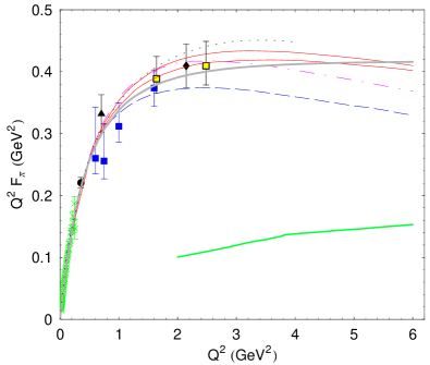
Figure 1: (color online). Our predictions for the pion form factor given in 1998 KrT01 (full red lines; upper line: wave functions (4), lower line: wave functions (5) with $n=3$ and (6)) compared with data and with some other models. Green crosses represent data points of Amendolia et al. Ame84 . Other data points (all taken from Ref. HuB08-2 ) are: reanalyzed points of Ackerman et al. Ack78 (full circle); reanalyzed points of Brauel et al. Bra79 (full triangle); JLab results (full diamond, blue and yellow squares). Other theoretical curves are: QCD approximation of Maris and Tandy MaT00 (dotted); perturbative QCD (leading and next-to-leading order) by Bakulev et al. BaP04 (green dash-dot-dotted); Nesterenko and Radyushkin NeR82 (magenta dash-dotted); dispersion approach of Donoghue and Na DoN97 (blue dashed); holographic approach of Grigoryan and Radyushkin GrR08 (thick grey).

Figure 2: (color online). Comparison of our predictions with other CQMs. Data and our curves are the same as in Fig. 1. Other theoretical curves are: those by C.-W. Hwang Hwa01 (blue dashed); Cardarelli et al. Car94 and (precisely coinciding with it) instant-form predictions HeJ04 (magenta dash-dotted); Ref. ChJ99 (green dotted). Predictions of an upgraded version of a seminal paper ChC88pl (Ref. CoP05 , Fig. 5, $m_{q}=0.22$) coincide precisely with our upper curve.

Let us note that our relativistic CQM describes well the experimental data for the pion form factor including the recent points HuB08-2 . The upper of our curves corresponds to the model (4), the lower - to the models (5) with $n=3$ and (6), which lie close to one another.

Let us emphasize that the parameters used in our calculations were obtained from the fitting to the experimental data up to $Q^{2}\;\simeq$ 0.26 GeV² Ame84 . At that time the data for higher $Q^{2}$ was not correlated in different experiments and had significant uncertainties. The later data for pion form factor in JLab experiments up to $Q^{2}$ =2.45 GeV² were obtained with rather good accuracy. All experimental points obtained in JLab up to now agree very well with our prediction of 1998.

Let us discuss briefly the basic moments that provide good results for the pion form factor in our approach. First, throughout the calculation the condition of Lorentz-covariance and the conservation laws for the operator of electromagnetic current were satisfied. Second, the condition of accurate description of the pion MSR constrains the behavior of the wave functions in momentum representation (4), (5) at small relative momentum of quarks or of the wave function in coordinate representation (6) at large distances because of special properties of the integral representation (1). Third, the condition of the best description of the decay constant defines constraints for the wave function at large relative momenta because the contribution of small relative momenta to the decay constant is suppressed as can be seen from the relativistic formula (see, e.g. KrT01 ; Jau91 ):

$$f_{\pi}=\frac{M\,\sqrt{3}}{\pi}\,\int\,\frac{k^{2}\,dk}{(k^{2}+M^{2})^{3/4}}\,u(k)\;.$$

So, our way of fixing the model parameters constrains effectively the behavior of wave functions both at small and at large relative momenta. The structure of our relativistic integral representation (1) is so, that the form–factor behavior in the region of small momentum transfers is determined by the wave function at small relative momenta, and the behavior of the form factor in the region of high momentum transfer — by the wave function at large relative momenta. The constraints for the wave functions provide the limitations for the form factor, and this is seen in the results of the calculation.

IV ASYMPTOTIC BEHAVIOR

It is worth to consider the form-factor asymptotic behavior at $Q^{2}\to\infty$ especially. In our paper KrT98tmph it was shown that in our approach, the pion form-factor asymptotics at $Q^{2}\to\infty$ and $M\to$ 0 does not depend on the choice of a wave function but is defined by the relativistic kinematics only. We consider the fact that the asymptotics obtained in our nonperturbative approach does coincide with that predicted by QCD as a very significant one. Our approach occurs to be consistent with the asymptotic freedom, and this feature surely distinguishes it from other nonperturbative approaches.

Let us note that it is obvious that at very high momentum transfers the quark mass decreases as it goes to zero at the infinity. Our approach permits to take into account the dependence $M(Q^{2})$ beginning from the range where this becomes necessary to correspond to experimental data. It is possible that this will take place at the values of $Q^{2}$ lower than $6$ GeV².

The correct asymptotics is the consequence of the fact that the relativism is an intrinsic property of our approach. To demonstrate how it works let us consider the simple example of point–like quarks and model wave functions (4). In this case in the Eqs. (1), (2):

$$G^{u}_{E}(Q^{2})+G^{\bar{d}}_{E}(Q^{2})=$$

$$=G^{u}_{M}(Q^{2})+G^{\bar{d}}_{M}(Q^{2})=1\;.$$

For the model (4) it is easy to obtain the non-relativistic integral representation of the form-factor as the corresponding limit of the Eq.(1). Now the integration can be performed analytically and the following form for the nonrelativistic pion form factor can be derived:

$$F_{\pi}(Q^{2})=\hbox{exp}\left(-\,\frac{Q^{2}}{16\,b^{2}}\right)\;.$$

One can see that in the non-relativistic case, the form factor does not depend on the mass of constituents and its asymptotics can not agree with that of QCD. The correct asymptotics is provided by relativistic effects.

In the relativistic case the results for the integrals can not be obtained analytically. To derive the asymptotic behavior in question it is possible to use the asymptotic series for double integrals obtained in Ref. KrT08 . The first two terms give:

$$F_{\pi}(Q^{2})\sim\frac{2^{5/2}M}{Q}\mathrm{e}^{-\frac{QM}{4b^{2}}}\left(1+\frac{7b^{2}}{2MQ}\right)\;.$$ (7)

Let us take in (7) the limit at $M/b\to 0$. This means that the parameters of the model are such that $M/b\ll 1$. The physical meaning of this limit is that the increase of the momentum transfer is followed by the “undressing” of the constituent quarks and its transformation into current quark of pQCD. In this limit we obtain from Eq. (7) up to logarithmic prefactors the power-like behavior coinciding with that of pQCD  KrT01 :

$$F_{\pi}(Q^{2})\sim\frac{14\sqrt{2}b^{2}}{Q^{2}}\;,$$

V SUMMARY

To conclude, we make some predictions about the results of the future JLab experiments on the pion form factor based on the method proposed in our papers earlier. The method is a variant of composite quark model in the instant-form of Poincaré invariant quantum mechanics. It is shown that our approach has certain advantages as compared with other CQM calculations. From a theoretical point of view, these advantages are the consequence of the fact that our approach has dispersion-relation motivated foundations. This provides, in particular, weak model dependence of the results of calculations. The approach has demonstrated earlier its predictive power in describing all the data on the pion form factor obtained later in JLab experiments. Our calculations also give the accurate values of the pion MSR and of the decay constant $f_{\pi}$, and the correct asymptotic behavior at $Q^{2}\to\infty$.

We hope that our model will provide a good description of the future JLab experiments on the measurement of the pion form factor in the range of momentum transfers up to $Q^{2}\approx 6$ (GeV)². If it will occur that beginning from some values one needs to adjust the calculations by introducing the quark mass dependence on $Q^{2}$ to agree the future data, then we propose to identify the effect with the appearance of perturbative effects.

This work was supported in part by the Russian Foundation for Basic Research (Grant No. 07-02-00962). The work of A.K. was supported in part by the Program ”Scientific and scientific-pedagogical specialists of innovative Russia” (Grant No. 1338).

References

- (1) H.P. Blok et al. (The Jefferson Lab Collaboration), Phys. Rev. C 78, 045202 (2008).
- (2) G.M. Huber et al. (The Jefferson Lab Collaboration), Phys. Rev. C 78, 045203 (2008).
- (3) G.M. Huber, D. Gaskell, JLab Proposal, E-12-06-101, “Measurement of the charged pion form factor to high ”, July 7, 2006.
-
(4)
H.P. Blok, G.M. Huber, and D.J. Mack,
“Measurement of th Charged Pion Form Factor to High
”, Contribution to Exclusive Reaction Workshop,
Jefferson Lab, May 2002,
nucl-ex/0208011 - (5) D. Ebert, R.N. Faustov, and V.O. Galkin, Eur.Phys.J.C 47, 745 (2006).
- (6) A.F. Krutov and V.E. Troitsky, Eur.Phys.J. C 20, 71 (2001), hep-ph/9811318.
- (7) J. Volmer et al., Phys. Rev. Lett. 86, 1713 (2001).
- (8) V. Tadevosyan et al., Phys. Rev. C 75, 055205 (2007).
- (9) T. Horn et al., Phys. Rev. Lett.97, 192001 (2006).
- (10) A.F. Krutov and V.E. Troitsky, Phys.Rev. C 65, 045501 (2002).
- (11) A.F. Krutov and V.E. Troitsky, hep-ph/0101327.
- (12) A.F. Krutov and V.E. Troitsky, Fiz. Elem. Chastits At. Yad. 40, 269 (2009) [[Engl. Transl. Physics of Particles and Nuclei, 40, 136 (2009)].
-
(13)
S.R. Amendolia et al.,
Phys. Lett. B146,116 (1984).
S.R. Amendolia et al., Nucl. Phys. B277, 168 (1986). - (14) B. Desplanques and Y.B. Dong, Eur. Phys. J. A37, 433 (2008).
- (15) Yu. M. Shirokov and V. E. Troitsky, Nucl.Phys.B 10, 118 (1969).
- (16) V. P. Kozhevnikov, V. E. Troitsky, S. V. Trubnikov, and Yu. M. Shirokov, Teor. Mat. Fiz. 10, 47 (1972) [Engl. Transl. Theor. Math. Phys. 10, 30 (1972)].
- (17) V.E. Troitsky, S. V. Trubnikov, and Yu. M. Shirokov, Teor. Mat. Fiz. 10, 209 (1972) [Engl. Transl. Theor. Math. Phys. 10, 136 (1972)] V.E. Troitsky, S. V. Trubnikov, and Yu. M. Shirokov, Teor. Mat. Fiz. 10, 349 (1972) [Engl. Transl. Theor. Math. Phys. 10, 234 (1972)]
- (18) A. I. Kirillov , V. E. Troitsky , S. V. Trubnikov , and Yu. M. Shirokov, Fiz. Elem. Chastits At. Yad. 6 ,3 (1975) [[Engl. Transl. Sov. J. Part. Nucl. 6, 3 (1975)].
- (19) V. E. Troitsky, in Quantum Inversion Theory and Applications, Proceedings, Germany, 1993, edited by H.V.von Geramb, Lecture Notes in Physics 427, 50 (Springer Verlag, 1994).
- (20) V. V. Anisovich, M. N. Kobrinsky, D. I. Melikhov, and A .V. Sarantsev, Nucl. Phys. B544 747 (1992).
- (21) D. I. Melikhov, Eur. Phys. J. direct C4 (2002) 2 [hep-ph/0110087].
- (22) A.F. Krutov and V.E. Troitsky, JHEP 10, 028 (1999).
- (23) A.F. Krutov, Yad. Fiz. 60, 1442 (1997) [Phys. At. Nuclei 60, 1305 (1997)].
- (24) V.A. Matveev, R.M. Muradyan, and A.N. Tavkhelidze, Lett. Nuovo Cim. 7 719 (1973).
- (25) S. Brodsky and G. Farrar, Phys.Rev.Lett. 31 1153 (1973).
- (26) A. Radyushkin, ”Quark Counting Rules: Old and New Approaches”, arXiv:0907.4585.
- (27) G. R. Farrar and D. R. Jackson, Phys. Rev. Lett. 43, 246 (1979).
- (28) A. V. Efremov and A. V. Radyushkin, Teor. Mat. Fiz. 42, 147 (1980) [Engl. Transl. Theor. Math. Phys. 42, 97 (1980)] Report JINRE2-11983, Oct. 1978, 32pp.
- (29) A. V. Radyushkin, hep-ph/0410276 JLAB-THY-04-35 October 20, 2004, JINR P2-10717 June 14,1977
- (30) F. Cardarelli et al., Phys. Lett. B332, 1 (1994); F. Cardarelli et al., Phys. Rev. D 53, 6682 (1996).
- (31) P.L. Chung. F. Coester, and W.N. Polyzou, Phys. Lett.B205 545 (1988).
- (32) F. Coester and W.N. Polyzou, Phys. Rev. C 71, 028202 (2005).
- (33) F. Schlumpf, Phys. Rev. D 50, 6895 (1994).
- (34) G.P. Lepage, S.J. Brodsky, Phys.Rev.D 22, 2157 (1980).
- (35) S.J. Brodsky, G.P. Lepage, Perturbative Quantum Chromodynamics. - Singapore: World Scientific Publishing, 1989. - 93 p.
- (36) H. Tezuka, J. Phys. A Math. Gen. 24, 5267 (1991).
- (37) Particle Data Group. Part II, Phys.Rev.D 45 (1992).
- (38) H. Ackermann et al., Nucl. Phys. B137,294 (1978).
- (39) P. Brauel et al., Z. Phys. C3, 101 (1979).
- (40) P. Maris and P.C. Tandy, Phys. Rev. C 62, 055204 (2000).
- (41) A.P. Bakulev, K. Passek-Kumericki, W. Schroers, and N. G. Stefanis, Phys. Rev. D 70, 033014 (2004), and erratum Phys. Rev. D 70, 079906 (2004)
- (42) V.A. Nesterenko and A.V. Radyushkin, Phys. Lett. B115, 410 (1982).
- (43) J.F. Donoghue and E.S. Na, Phys. Rev. D 56, 7073 (1997).
- (44) H. V. Grigoryan and A. V. Radyushkin, Phys. Rev. D 78, 115008 (2008).
- (45) C.-W. Hwang, Phys. Rev. D 64, 034011 (2001).
- (46) Jun He, B. Juliá-Díaz, and Yu-bing Dong, Phys.Lett. B602, 212 (2004).
- (47) H.-M. Choi and C.-R. Ji, Phys. Rev. D 59 074015 (1999).
- (48) W. Jaus, Phys.Rev.D 44, 2851 (1991).
- (49) A. F. Krutov and V. E. Troitsky, Teor. Mat. Fiz. 116, 215 (1998) [Engl. Transl. Theor. Math. Phys. 116, 907 (1998)].
- (50) A.F. Krutov, V.E. Troitsky and N.A. Tsirova, J. Phys. A: Math. Theor. 41, 255401 (2008).