The Effect of Differential Limb Magnification on Abundance Analysis of Microlensed Dwarf Stars

Abstract

Finite source effects can be important in observations of gravitational microlensing of stars. Near caustic crossings, for example, some parts of the source star will be more highly magnified than other parts. The spectrum of the star is then no longer the same as when it is unmagnified, and measurements of the atmospheric parameters and abundances will be affected. The accuracy of abundances measured from spectra taken during microlensing events has become important recently because of the use of highly magnified dwarf stars to probe abundance ratios and the abundance distribution in the Galactic bulge. While the abundance ratios in general agree with the giants, with the possible exception of [Na/Fe], there may be more dwarfs than giants with high [Fe/H]. In this paper, we investigate the effect of finite source effects on spectra by using magnification profiles motivated by two events to synthesize spectra for dwarfs between 5000K to 6200K at solar metallicity. We adopt the usual techniques for analyzing the microlensed dwarfs, namely, spectroscopic determination of temperature, gravity, and microturbulent velocity, relying on equivalent widths. We find that ignoring the finite source effects for the more extreme case results in errors in T_eff$<45$K, in log $g$ of $<$0.1 dex and in $\xi$ of $<$0.1 km/s. In total, changes in equivalent widths lead to small changes in atmospheric parameters and changes in abundances of $<$0.06 dex, with changes in [Fe I/H] of $<$0.03 dex. For the case with a larger source-lens separation, the error in [Fe I/H] is $<0.01$ dex. This latter case represents the maximum effect seen in events whose lightcurves are consistent with a point-source lens, which includes the majority of microlensed bulge dwarfs published so far.

1. Introduction

A microlensing event occurs when a stellar mass object passes between the observer and a background source. For events in the Local Group, the source is a star. If the source is finite, rather than infinitely small, parts of the source may be magnified more than other parts. In the case of stars, for example, the limb can be brightened relative to an unmagnified source. Since the light from the limb comes from different temperature profiles in the star compared to the center, this will affect the spectrum (e.g. Valls-Gabaud, 1995; Loeb & Sasselov, 1995) For example, a spectrum of the limb of the Sun has Balmer lines with weaker wings, while lines of other elements can be either weakened or strengthened relative to the center (Hastings, 1873; Hale & Adams, 1907).

Recently, observers using large telescopes have published abundance ratios in dwarfs in the Galactic bulge from spectra obtained while the sources were highly magnified. A number of these have turned out to have super-solar metallicities, including OGLE-2006-BLG-265S (Johnson et al., 2007), MOA-2006-0BLG-099S (Johnson et al., 2008), OGLE-2007-BLG-349S (Cohen et al., 2008), MOA-2008-BLG-310S and MOA-2008-BLG-311S (Cohen et al., 2009) and OGLE-2007-BLG-514S (Epstein et al., 2009). Some are metal-poor including the subgiant OGLE-2008-BLG-209S (Bensby et al., 2009a) and the dwarf OGLE-2009-BLG-076S (Bensby et al., 2009b), which, at [Fe/H]$=-0.76$ is the most metal-poor dwarf/subgiant observed when microlensed. For a sample of eight microlensed dwarfs, Epstein et al. (2009) found that a K-S test gave a 1.6% chance that the dwarfs were drawn from the same metallicity distribution function (MDF) as the giant MDF from Zoccali et al. (2008). Bensby et al. (2009c) report results for a total of 13 dwarfs, including new results for more metal-poor dwarfs, so clearly the comparison between the giants and the dwarfs is an evolving topic. Cohen et al. (2008) proposed that mass-loss on the giant branch prevents some more metal-rich stars from becoming red giants, similar to the mechanism suggested by Kalirai et al. (2007) to explain the low-mass He white dwarfs in the metal-rich cluster NGC 6791. However, this explanation predicts that the red clump MDF is biased to more metal-poor stars because of metal-rich stars skipping the horizontal branch phase and that the red giant luminosity function should drop more than expected from theoretical models, predictions that do not agree with the giant data (Zoccali et al., 2008). Another explanation is that there are systematic differences between giant and dwarf abundance analyses. Cohen et al. (2009) calculated that a systematic offset of 0.10 dex between the dwarf and giant metallicity scales would give the mean metallicity offset a significance of 2-$\sigma$ and larger systematic offsets would obviously decrease the significance further still. Finally, Zoccali et al. (2008) suggested that the spectra of microlensed dwarfs could be affected by differential magnification sufficiently that the usual analysis of the dwarfs, which does not take this into account, could lead to biased answers and help explain the possible discrepancy. This last suggestion can be tested by comparing the answers obtained from synthetic spectra with and without differential limb magnification.

While most microlensing events follow the lightcurve of a point source, about $\sim$3% (Witt, 1995) of events show finite source effects. This fraction is even higher for high-magnification events that are targets of the current generation of dwarf studies. Of the eight published events for which dwarf spectra were obtained, we know that at least three of the events were affected by finite source effects, namely OGLE-2007-BLG-514, OGLE-2007-BLG-349, and MOA-2008-BLG-310. We need to determine the size of the effect that differential limb magnification (DLM) has on the spectra and the measurement of the effective temperature (T_eff), gravity (log $g$), metallicity ([Fe/H]), microturbulent velocity ($\xi$) and abundance ratios to correctly interpret these events.

In addition to probing the chemical evolution of the bulge, the accuracy of the measured T_eff from the spectrum is important for testing the method by which colors of source stars in microlensing events are determined. Using a metallicity and a T_eff derived from the spectrum, we can predict the color of the star using relations between color and T_eff, such as that by Ramírez & Meléndez (2005), and compare with the color estimated using standard microlensing techniques, which rely on the offset of the star from the red clump. The results so far indicate that if the color of the red clump is $(V-I)_{0}$=1.05, the T_effs derived spectra are in agreement with T_effs from colors.

Much work has been done on the effects of DLM of the disk of giants during a microlensing event because these events are easier to find and are longer-lasting than similar events in dwarfs. Valls-Gabaud (1998) predicted the effects on the spectrum of a giant, in particular the H$\beta$ and CO lines, by fitting simple analytic expressions to the limb profiles for both continuum and lines from the Kurucz (1992) models. He found that the equivalent widths could change by 20% over the course of the event. Heyrovský et al. (2000) computed more realistic models avoiding the use of linear approximations. They calculated contribution functions for lines, which indicate where the lines are formed, and illustrated the range of behavior individual spectral features will have because of varying center-to-limb profiles. Gaudi & Gould (1999) pointed out that binary lens events had particular advantages for resolving stellar surfaces, for example the fact that the second caustic crossing can be predicted if the event is monitored, and therefore carefully observed.

Thanks to intensive monitoring by observers, the effect of the size of the source on microlensing events has been observed many times. Finite source effects were observed for the giant MACHO 95-30 (Alcock et al., 1997), including variations in the equivalent widths of H$\alpha$ and the TiO bands. The bulge K3 giant star EROS BLG-2000-5S was highly magnified by a binary lens. Because the caustics of a binary lens are symmetric, the timing of the second caustic crossing was predicted to high accuracy and allowed intensive follow-up during this event. Both Albrow et al. (2001) and Castro et al. (2001) found decreases in the strength of the H$\alpha$ line when the limb was more highly magnified relative to the center. Afonso et al. (2001) monitored the same event photometrically, measured the color of the limb, and found that the outer 4% of the limb showed strong H$\alpha$ emission, which they ascribed to the presence of a chromosphere. Albrow et al. (1999) performed the first limb-darkening measurement of a bulge giant for the event MACHO 1997-BLG-28, using photometry in the $V$ and $I$ bands. Other limb-darkening measurements were done for giants including MACHO 1997-BLG-41 (Albrow et al., 2000), and OGLE-2002-BLG-069S (Kubas et al., 2005), which the authors found agreed with a linear limb-darkening law. An opposite result was found by Cassan et al. (2006) who obtained photometry for the K giant OGLE-2004-BLG-254S and derived limb darkening coefficients in the $I$ and $R$ bands. Combining these results with other microlensed-based limb darkening measurements of K giants and comparing them to the predictions of ATLAS9 models, they found a disagreement, which they suggested was the result of the inadequacy of the linear limb darkening law. Time-resolved spectra of OGLE-2002-BLG-069S, a G5III star, by Cassan et al. (2004), showed the power of this technique for probing the stellar atmosphere. In this case, the changes during the event in wings of H$\alpha$ line, which are formed deep in the atmosphere, agreed with model predictions while the core of the line showed an emission peak, which again can only be explained by a chromosphere. That the temperature structure in the outer layers is not well understood for this event was also found by the analysis of Thurl et al. (2006). These studies show the potential to investigate the atmospheric structure of giants.

Studies of dwarf stars have been much rarer. Afonso et al. (2000) and Abe et al. (2003) reported the only measurements of limb darkening in dwarfs, for MACHO 98 SMC-1, a main-sequence A star and MOA 2002-BLG-33S, a solar-type star, respectively. The most relevant work to this paper is the analysis of Lennon et al. (1996) of the event MACHO 96-BLG-3. They took three exposures when the source, a dwarf star, was moving across a caustic. These R$\sim$1100 spectra with signal-to-noise (S/N) of 25-100 did not show any convincing cases of profile variability. Lennon et al. (1996) compared the observations of this star with both a library of high-resolution, high S/N spectra of F and G stars observed at Calar Alto and a grid of synthetic spectra, and derived stellar parameters of T_eff=6100K from the H$\alpha$ line, log $g$=4.25 from the Mg I triplet and a metallicity ([M/H]) between 0.3 and 0.6 from fits to regions with many Fe I and Ca I lines. They calculated the expected deviations from the unmagnified spectrum for this event, and found that the expected change in the line profiles for the three spectra was $\leq$ 1%, while the expected change in the continuum was $\leq$ 2%. Given the small changes expected and the S/N of the spectra, it is not surprising that no changes were observed, and that the derived atmospheric parameters of the star would also not be affected. Indeed, it is not surprising that most changes are small. The amount of magnification depends on the distance from the lens, but the emitted spectrum is the same for an entire annulus (for a spherical star). Because the distance from the lens varies around the annulus, the average magnification of a spectrum at a particular annulus is smaller than the largest magnification of an particular spot would suggest. In addition, while the spectrum of the star increasingly changes from center to limb, the intensity of the limb is lower than the center, by factors of a few. Therefore it is difficult to overcome the influence of the light coming from the central regions of the star in the disk-averaged light.

The work discussed above focused on learning about the atmosphere of the star and showed that finite source effects cause changes in the spectrum of the star, which can be inverted to give temperature as a function of depth. Because the same effects that make these extreme events interesting as probes of the atmosphere will also change the spectrum that is analyzed for elemental abundances, the goal of this paper is to determine the effect of DLM on the T_eff, $\xi$, log $g$, [Fe/H] and abundance ratios using the standard spectroscopic techniques, such as equivalent width analysis. Therefore, we will be concerned with mimicking standard abundance analysis as closely as possible, rather than exploring the full range of knowledge that can be gleaned from time-resolved spectroscopy of microlensed events.

2. Magnification Profiles during Microlensing Events

Our work was motivated by two events, MOA-2008-BLG-310 and OGLE-2007-BLG-514, which are illustrations of the kind of effects seen. For MOA-2008-BLG-310, the lens did in fact transit the source, and there were small perturbations during this transit caused by a planetary companion in the lens (Janczak et al., 2009). However, the spectrum analyzed by Cohen et al. (2009) began at UT 22:51, which was 21 minutes after the end of the transit, when the lens and source center were separated by $z=1.22$ source radii. Figure 1 shows the annulus-averaged profiles for a point lens at 15 minute intervals for the MOA-2008-BLG-310 geometry, beginning at $z=1.2$ and continuing as the lens and source moved further apart. The magnification is given as a function of $\theta$, which is the angle between the normal to the stellar surface and the line of sight to the observer. To determine This look at the later stages of MOA-2008-BLG-310 will be referred to as Event A. The start time for the first profile is three minutes before the Cohen et al. (2009) observations began, and thus serve as a direct measurement of the size of the effect of DLM on those abundances, but they also serve a broader purpose.

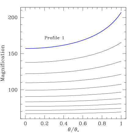
Figure 1.— Differential limb magnification profiles for Event A. The bold line shows Profile 1, which represent the most extreme differential magnification for this event, and is the profile from the first 15 minutes of Event A. At most, the limb is magnified by $\sim 30\%$ more than the center.

In this particular case, we know that $z=1.22$ at the time of the observations because the source size was earlier detected by observations (from Africa) of a direct source crossing. However, if the closest separation between source and lens during the entire event (i.e., the impact parameter) had been $z_{0}=1.22$, there would have been no source crossing at any time. If the impact parameter is sufficiently large, then it becomes impossible to determine the source radius from the lightcurve. In such a case, only upper limits can be placed on the magnitude of DLM and profiles of the DLM as a function of $\theta$ cannot be derived.

However, for $z_{0}\leq 1.2$, the effects of the finite-source size on the light curve are sufficiently pronounced to measure $z_{0}$. Thus, the top curve in Figure 1 represents the most extreme case of DLM that would occur without being noticed, and thus serves as a general check on ignoring DLM when it is not detectable from the light curve.

The other case represents a more extreme event, inspired by OGLE-2007-BLG-514, and will be called Event B. Here, the source trajectory crossed a cusp from a binary lens and produced extreme magnification variations (Figure 2). Once the parameters are selected, it is straightforward to compute the magnification at each time and for every point on the source plane. We calculated the mean magnification in concentric rings with annuli equal to 0.01 source radii using the “loop-linking” technique (Dong et al., 2006). The profiles are spaced at five minute intervals for this event. Actual observations are always longer, usually 5-6$\times$ longer in order to get enough S/N in each exposure to reliably extract the spectrum. Spectra at 5 minute intervals could only be obtained for dwarfs magnified to apparent magnitudes that have not been seen in an event to date, so in reality microlensing spectra will smear out these profiles and dilute their effects. Figure 3 shows 51 different profiles that occurred during this event. We note that in this case we have ample notice from the lightcurve that finite source effects are important and we could use that information to derive the magnification profile at the time spectra were taken and make model spectra that include the effects of DLM. However, in this paper, we consider the cases that ignored finite source effects on the spectrum to measure the size of errors that this induces on the parameters, metallicities and abundance ratios.

Figure 2.— The top panel shows, for Event B, the source-averaged magnification as a function of time, measured in units of the source-radius crossing time. The bottom panel shows the geometry of the event at a moment when the source (circle) is just exiting the caustic (acute-angled structure), which is a contour of formally infinite magnification. The source-center position is marked by small circles at 5 minute intervals. As the source passes over the caustic, it is differentially magnified, with first the limb, then the center, and finally the limb being the most magnified.

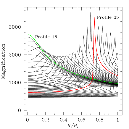
Figure 3.— The magnification of the disk of a dwarf as a function of radius at each interval marked in Figure 2. We see in the most extreme cases that parts of the disk are magnified up to 5$\times$ more than other parts. The two profiles that are examined in more detail in the text are for time step 18 (bold line peaking at $\theta=0$) and time step 35 (bold line peaking at $\theta=0.75$)

3. Synthesized Spectrum

We explored the changes to the spectra of dwarfs caused by the magnification profiles given in §2. We interpolated a set of model atmospheres from the Kurucz-Castelli grid with new opacity distribution functions (Castelli & Kurucz (2003) . The models are solar-metallicity and are spaced every 100 K from 5000K to 6200K. This temperature range covers the range of temperatures for dwarfs observed in the bulge. Cooler dwarfs ($<5000$ K) are unlikely to ever be targeted because of their intrinsic faintness and because if the dwarfs are as cool as the giants, many of the advantages of measuring abundances in dwarfs rather than giants (such as reduced blending) no longer apply. Although the majority of the bulge population is old (Ortolani et al., 1995), we wanted to explore a large temperature range of main-sequence/main-sequence turnoff stars, and therefore we adopted log $g$ values from a Yale-Yonsei isochrone (Yi et al., 2001) of 4 Gyr. At this age, stars with T_eff=6000K have two possible values for log $g$, because they are at the turnoff, while dwarfs with 6100K and 6200K are still present because of the blue hook in the isochrone. The two 6000K dwarfs allow us to measure the effect that small changes in log $g$have on the resulting spectra. Table 1 lists the temperatures and log $g$’s for the dwarfs.

Table 1Parameters for Model Atmospheres

Teff(K)	log $g$	[Fe/H]	$\xi$ (km/s)
5000	4.60	0.00	1.500
5100	4.59	0.00	1.500
5200	4.57	0.00	1.500
5300	4.55	0.00	1.500
5400	4.53	0.00	1.500
5500	4.51	0.00	1.500
5600	4.48	0.00	1.500
5700	4.46	0.00	1.500
5800	4.43	0.00	1.500
5900	4.39	0.00	1.500
6000	4.33	0.00	1.500
6000	4.06	0.00	1.500
6100	4.01	0.00	1.500
6200	3.98	0.00	1.500

3.1. Method of Synthesizing Spectra

We focused our attention on three 200 Å sections of the spectrum, centered on H$\alpha$ (6460 Å– 6660Å), H$\beta$(4757Å– 4957Å) and the Mg I triplet (5067 Å– 5267 Å). These regions have both strong lines, which are expected to show the largest variations, as well as a number of weaker lines whose equivalent widths would be used in an abundance analysis. The wavelength range from blue to red also ensures that detectable unblended lines can be found for both cooler stars, which have crowded blue regions, and hotter stars, which tend to have weak lines in the red. The H$\alpha$ and H$\beta$ lines are also used as a temperature indicator in hotter dwarfs. For each model atmosphere, we used Turbospectrum (Alvarez & Plez, 1998) to generate intensities I($\theta$) at 100 values of $\theta$. To determine the total flux from the star, we added up the intensities coming from annuli from the center to the radius R of the star

$$F=2\pi\int_{0}^{R}I(\theta)rdr$$ (1)

(see e.g., Mihalas, 1978) Using $r=Rsin\theta$, for the unmagnified case, the observed flux can be obtained by numerical integration of the equation

$$F=2\pi\int_{0}^{\frac{\pi}{2}}I(\theta)cos\theta sin\theta{\mathrm{d}}\theta$$ (2)

This gives the same answer as when Turbospectrum outputs a flux, rather than intensities. For the magnified cases, each annulus was multiplied by its magnification factor before integration. The spectra were smoothed to a FWHM of 0.11Å, or R$\sim$ 45,000, similar to the resolution at which the dwarfs are observed.

3.2. Comparison of Spectra

To investigate the size of possible systematic effects on the abundances in dwarf stars, we wished to determine the maximum effect on the spectroscopic analysis, and therefore begin by identifying the cases for which the spectra deviate the most from the unmagnified case. We took the ratio between the magnified and the unmagnified spectra, renormalized the spectra and then calculated the rms.

For Event A, neither the profiles nor the rms varies much, but the largest deviations are found for the profile calculated for the first time step, indicated by the bold line in Figure 1. For Event B, the rms is highest, as expected, when the limb is magnified by a high factor or when the center region is magnified the most (bold lines in Figure 3). These occur for the 18th and 35th profiles calculated, corresponding to 85 and 170 minutes after Event B began. We will use these three profiles as examples to calculate the size of the effects on the abundances. The indicated case from Event A will be called Profile 1 and the two indicated cases from Event B will be called Profile 18 and 35.

Figure 4 illustrates the changes to a spectrum by showing the ratio of the unmagnified spectrum to the spectra created using the three different magnification profiles for the 5500K dwarf. The changes are small, but vary from line-to-line based on the location of the line-forming region. In general, the strong lines, including H$\alpha$ and H$\beta$, become weaker for Profiles 35 and 1, for which the limb is magnified relative to the center, while the reverse is true for the spectrum from Profile 18. The opposite behavior is seen for most of the weak lines. As expected, the deviations are largest for the two cases where the magnification profile is more extreme and much smaller for Event A, where the differential magnification effects were $\sim 30\%$, rather than $\sim 500\%$.

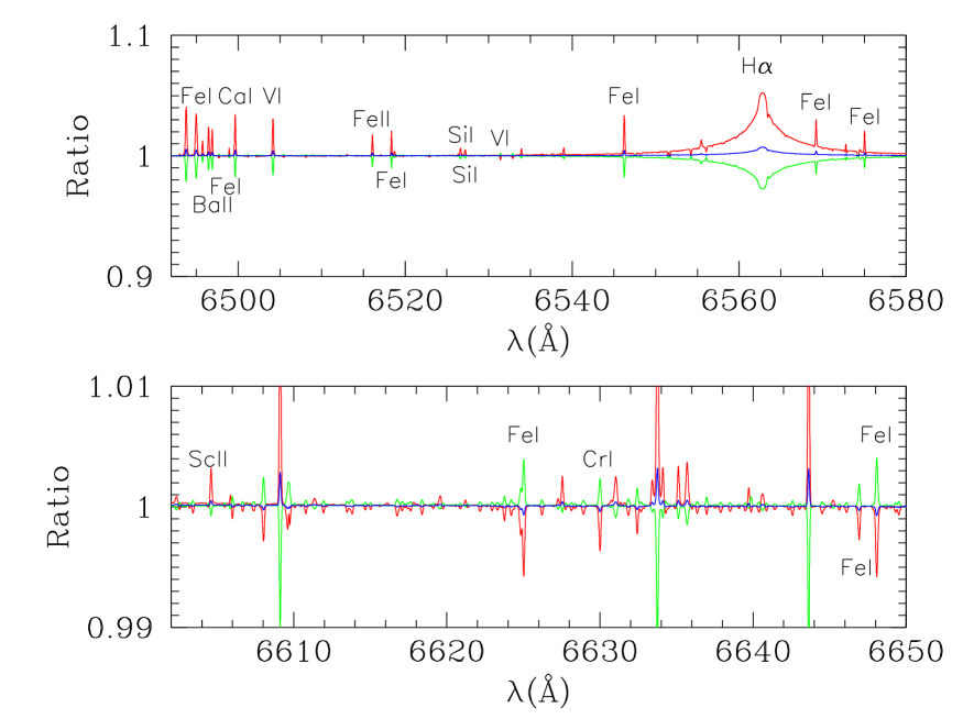
Figure 4.— Ratio of the spectra in the magnified cases to those in the unmagnified case for the 5500K model. The red line is for Profile 35, the green line for Profile 18 and the blue line is for Profile 1. Top: part of the H$\alpha$ spectrum, showing the stronger lines tend to be weaker for Profile 35 than for Profile 18, and in both cases the effects are much stronger than for Profile 1. Bottom: part of the H$\alpha$ spectrum, focusing on weaker lines, which tend to be weaker for Profile 18 than for Profile 35. Again, Profile 1 shows the smallest effects.

4. Abundance Analysis

The goal of this paper is to determine the practical effect of finite source effects on abundance measurements in microlensed dwarfs. To do this, we followed the usual steps used to analyze these spectra. Because differential reddening across the face of the bulge leads to uncertainty in the colors and magnitudes of stars in the bulge, analyses of microlensed dwarfs have relied on spectroscopic methods of deriving atmospheric parameters, rather than color or apparent magnitude-based methods. DLM can impact the derived abundances in the source star by changing the EWs of the lines and by changing the atmospheric parameters derived from those EWs. To examine these effects and compute the total effect of DLM on the abundances, we first measured EWs in the synthetic spectra for the unmagnified case and Profiles 18, 35 and 1. We ran all sets of EWs through the original model atmosphere to see what changes. We found small changes in the diagnostics used to determine T_eff, log $g$, and $\xi$, in addition to changes in the abundances. We first discuss the magnitude of the changes demanded by the magnified spectra on the atmospheric parameters, considering each one in isolation. While the exact magnitude of the changes depends in detail on which lines are used for any particular study, the results here will give a general indication. Looking at the changes in each parameter separately shows the size of the effect if only some of the parameters are determined from the spectra. However, because deriving the atmospheric parameters usually depends on the other parameters, we next consider the total effect of the accumulated atmospheric parameter changes plus EW changes. Once again, depending on the line list used, different correlations between the parameters may be found, but the overall tendencies can be generalized.

4.1. Equivalent Width Measurement

In measuring EWs on the model spectra, we encountered the same concerns about continuum placement and blending as in measuring EWs on observed spectra. Because of our desire to determine differences caused by differential limb magnification, we focus on measuring EWs in a consistent manner. We first used IRAF to do the continuum division, keeping the parameters of the fit, such as the order of the polynomial and the high and low-reject sigmas, the same for both magnified and unmagnified spectra. Then we measured the EWs without adjusting the continuum interactively, using SPECTRE (C. Sneden, 2007, private communication) to fit Gaussian profiles to the spectra. Our initial linelist was selected using the solar atlas of Moore et al. (1966) as a guide to unblended lines, but this was not completely foolproof at the lower resolution (compared to the solar atlas) of the synthesized spectra, and over the large temperature range spanned by the models. Therefore we checked the list by determining the abundances from the lines for the unmagnified spectra. Any line that deviated by more than 0.1 dex from the mean is eliminated. Also eliminated are lines with EW $>150$mÅ in the unmagnified case, because these lines are usually eliminated in high-resolution analysis due to their sensitivity to damping parameters, continuum placement, blending in the wings and incorrect temperature structure in the outermost layers of the model atmospheres. For each temperature, the same lines were measured for each magnification profile; however, because the strength of lines varies with temperature, the linelist changes for different temperatures. Because the same transition information, such as $gf$-value, was used both to synthesize the spectra and to calculate the abundance, there are no uncertainties introduced in this process by atomic data uncertainties.

In Figure 5, we compare the difference in EWs for the three magnification profiles under study. We find that, as expected, the smaller differences between limb and center for Profile 1 result in smaller changes in the EWs. As seen in Figure 4, weaker lines are mostly strengthened and strong lines mostly weaken for Profile 35, while the opposite is true for Profile 18. This emphasizes the point that the magnitude of the changes for a particular analysis will depend on the distribution of EWs that are being used. We then ran the EWs through Turbospectrum, using the original model atmosphere. This comparison isolates the effect of the EW changes on the abundances, before we consider changes caused by new atmospheric parameters, and would reflect the total changes if the analysis relied on non-spectroscopic methods for atmospheric parameter determination, such as color of the unmagnified star for T_eff and position on the CMD for gravity. The changes in abundances are shown in Figure 6, and show the magnitude of $\delta$ log$\epsilon$ is generally ¡ 0.05 dex.

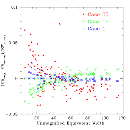
Figure 5.— A comparison of the EWs measured in the magnified spectra to those in the unmagnified spectrum for the 5500K model.

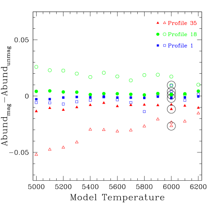
Figure 6.— The change in Fe I abundances (filled symbols) and Fe II abundances (open symbols) that result from changes in the EWs alone. Different linelists and continuum division for different temperature models lead to more bumpiness in the relation with temperature than otherwise. Large circles show the lower gravity 6000K model points. Overall, it is clear that the changes in the EWs in themselves do not result in large changes to the abundances. For Profile 18, for which the center was magnified more than the limb, analyzing the EWs assuming the unmagnified model results in a increase of the derived metallicity, while the reverse is true for Profile 35. Very small changes are seen for Profile 1, as expected given the small deviations seen in Figure 4

4.2. T_eff

There are two standard ways of determining the temperature of a star from its spectrum, without relying on its color. The first uses the wings of the Balmer lines, while the second requires excitation equilibrium for Fe I, so that there is no trend in a plot of lower excitation potential to abundance derived for each line.

H$\alpha$ is well-known to show the effects of DLM. Figure 7 compares the H$\alpha$ profiles of the unmagnified case to the most extreme magnified cases (Profile 18 and 35) for the T_eff=5500K model. It is clear that the H$\alpha$ profiles are different in the magnified models, and a different temperature would be derived if DLM were not taken into account. By comparing the magnified cases with the unmagnified profiles of the different temperature models, we determine that the T_eff we would derive would be 75K or 100K hotter for Profile 18 and would be 75K or 100K cooler for Profile 35. This is consistent with the magnification profiles for these two cases, because Profile 18 has the center, where we see to hotter temperatures, magnified more than the limb, while the opposite is true for Profile 35.

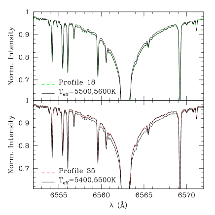
Figure 7.— Comparison of unmagnified spectrum at H$\alpha$ with magnified spectra for Profile 18 (top) and Profile 35 (bottom). The magnified cases are shown for T_eff=5500K. In the top panel, the unmagnified cases shown are for T_eff=5500K and T_eff=5600K. The slightly broader wings from the Profile 18 spectrum show that we would calculate a higher temperature ( 100K) from this spectrum if we ignored DLM. This agrees with the larger contribution from the center of the star, because its spectrum features stronger Balmer lines. In the bottom panel, the unmagnified cases shown are for T_eff=5500K and T_eff=5400K. Here we would have calculated a lower temperature, which is in agreement with the prominence of the limb, with its weaker Balmer lines, in this particular profile.

Determining the temperature via the wings of the H$\alpha$ line requires high S/N data and becomes increasingly difficult at lower temperatures. Therefore, the more common method, used by all the papers on microlensed dwarfs discussed in the Introduction, is excitation equilibrium. We found that the slope of the line, determined by a least-squares fit, in the excitation potential-log$\epsilon$(Fe) plane changes if we used the EWs measured from the DLM spectra. Because of errors in continuum division and blending, the slope of the line in the unmagnified case, which theoretically should be zero, deviates slightly from that value. Therefore, to calculate the change in T_eff from this method caused by the effects of DLM on the spectrum, we calculated the change in temperature needed to get the slope back to that measured in the unmagnified case. Because we found the temperature shifts are small, we ran a series of model atmospheres with the temperature decreased by 25K, found the new slope using the magnified EWs, and used the results to calculate the necessary temperature change. The results are illustrated in Figure 8. We also did the test with +25 K and got the same answer to within 1 degree.

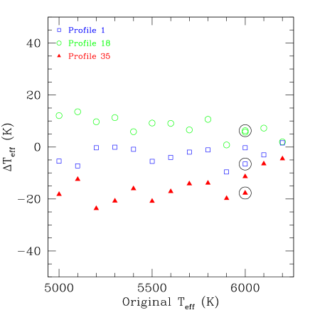
Figure 8.— The change in T_eff required to obtain the same excitation equilibrium as in the unmagnified case. Profile 18 requires higher temperatures, because the center is magnified relative to the limb, while Profiles 35 and 1 require lower temperatures. Overall, the temperature changes are larger at lower temperatures. Large circles mark the lower gravity 6000K model. The original gravity of the star makes only a very small difference.

4.3. Microturbulent Velocity

The microturbulent velocity is determined for 1-D analysis by ensuring that the slope for the derived abundance as a function of reduced EW for lines of an element is zero. Usually, the large number of Fe I lines make it the element of choice for this test, and this was the case for the analyses of the microlensed dwarfs. We compared the slopes of the lines in the Fe I vs. reduced EW (RW) plot in the magnified case to that in the unmagnified cases using the Fe abundances determined with the original model atmosphere in both cases. There is a change in the slope of the line in the magnified cases, because their EWs are affected by DLM.. As with the T_eff, the slope of the line in the unmagnified case is not exactly zero. We run our EWs and original model atmospheres through Turbospectrum, this time with $\xi$ set to 1.4 km/s and use the change in the slope for 0.1 km/s to interpolate the change in $\xi$. The magnitude of the change is always $<0.1$ km/s (Figure 9).

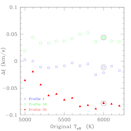
Figure 9.— The changes in $\xi$ necessary to have the slope in the RW/Fe I plane be the same as in the unmagnified case for which only $\xi$ is allowed to change. Large circles mark the lower gravity 6000K model.

4.4. log $g$

For the analysis of the microlensed dwarfs, gravity is determined spectroscopically by demanding that Fe I and Fe II (or other ions) give the same abundance. Obviously, changes in the EWs of these lines as well as changes in T_eff and $\xi$ will result in a change in the derived log $g$. In Figure 10, we show the changes in log $g$ that are necessary to get agreement between Fe I and Fe II considering the changes in EW alone.

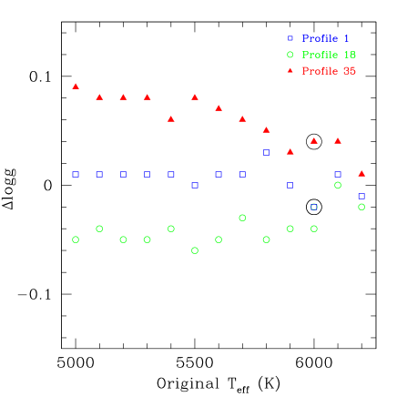
Figure 10.— The changes in log $g$ for each model necessary to bring Fe I and Fe II back into agreement, keeping the temperature at the original temperature and $\xi$ at the original $\xi$. Large circles mark the lower gravity 6000K model.

4.5. Abundances

In the previous subsections, we have considered the changes necessary in T_eff, $\xi$ and log $g$ if we kept the other parameters equal to those of the original model and only modified the one under consideration. This is appropriate when one model atmosphere parameter is chosen independently of the others. However, when deriving a model atmosphere, changes in one parameter will usually propagate and lead to total changes that can be larger or smaller than the partial derivatives suggest. In this section, we now consider the total effect on the calculated abundances, both from all the correlated changes in determining of the model atmosphere parameters and also from the changes in the EWs of the elements being measured.

For our particular linelist, T_eff, log $g$ and $\xi$ all affect the slope of the excitation potential vs. Fe I abundance plot, the slope of the reduced equivalent width vs. Fe I abundance plot and the difference in abundance between Fe I and Fe II lines. Therefore, using the partial derivatives we calculated above, we simultaneously solve for the changes in T_eff, log $g$ and $\xi$ that resulted in the slopes of the two lines and the difference in the two ions being the same as in the unmagnified case. The changes in the atmosphere models from the original parameters in Table 1 are listed in Table 2. The changes are given as magnified parameters $-$ unmagnified parameters. Finally, we interpolated a model with those parameters and run the EWs through that model to calculate the final change in the abundances. We checked that the final model has the excitation, equivalent width and ionization equilibrium to within the scatter (e.g., ¡ 0.01 dex difference in ionization equilibrium) expected considering the effects of rounding off temperatures, gravities and velocities. As these are interpolated models to begin with, these changes will never be that precisely determined. We note that the metallicity of the model atmosphere will have an effect on the abundances. However, the changes in log$\epsilon$(Fe) based on Fe I lines, which is how the metallicity of the atmosphere is usually set, are small enough that we will ignore this last effect for the purposes of the paper. For example, the change of 0.02 dex in Fe I for the 5600K model with Profile 35 would lead to a subsequent change for 0.006 dex in Fe I if folded back into a new model. Of course, the detailed analysis of a particular event could take these into account.

Figure 11 shows the resulting changes in the log$\epsilon$ for the elements considered here for 5000K, 5600K and 6200K. This figure illustrates the small magnitude of the changes expected from DLM in the dwarfs. Also, the changes in abundances are not always in the same sense. Depending on what part of the source is most highly magnified, the change caused by not taking DLM into account can either be an increase or decrease over the true abundances in the star. For some ions, such as Fe II, the changes using the new parameters are smaller than using the new EW with the unmodified atmosphere (seen by comparing Figure 6 and Figure 11). For others, such as Fe I, the changes with the new parameters are larger than seen just using the new EWs.

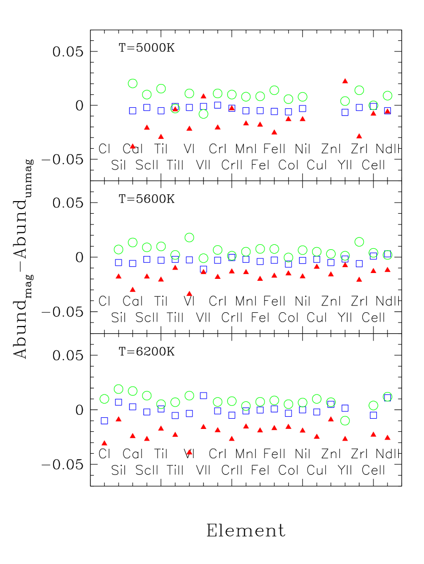
Figure 11.— The change in abundance (unmagnified-magnified) from the unmagnified case for three profiles studied in detail in this paper. Top: 5000K model Middle: 5600K case Bottom: 6200K case. Not all elements were measured for each temperature. We see that when DLM is not taken into account when analyzing the spectrum, the abundances can be in error by up to 0.05 dex.

Table 2Changes in Parameters for Magnified Model Atmospheres

Profile	$\Delta$Teff	$\Delta$log $g$	$\Delta$ [Fe/H]	$\Delta\xi$
Original Teff=5000K
Profile 1	$-$4.0	$-$0.006	$-$0.005	0.002
Profile 18	23.5	0.024	0.008	0.031
Profile 35	$-$40.3	$-$0.039	$-$0.018	$-$0.059
Original Teff=5100K
Profile 1	$-$4.7	$-$0.006	$-$0.005	0.002
Profile 18	23.8	0.028	0.008	0.036
Profile 35	$-$31.9	$-$0.010	$-$0.015	$-$0.047
Original Teff=5200K
Profile 1	$-$5.6	$-$0.005	$-$0.001	$-$0.013
Profile 18	21.7	0.025	0.007	0.035
Profile 35	$-$39.6	$-$0.046	$-$0.008	$-$0.048
Original Teff=5300K
Profile 1	$-$4.7	$-$0.005	$-$0.001	$-$0.013
Profile 18	20.6	0.025	0.008	0.032
Profile 35	$-$40.2	$-$0.049	$-$0.018	$-$0.065
Original Teff=5400K
Profile 1	$-$4.5	$-$0.007	$-$0.003	$-$0.010
Profile 18	20.8	0.022	0.005	0.041
Profile 35	$-$36.9	$-$0.055	$-$0.017	$-$0.059
Original Teff=5500K
Profile 1	$-$4.4	$-$0.016	$-$0.001	$-$0.003
Profile 18	19.8	0.020	0.007	0.039
Profile 35	$-$34.5	$-$0.060	$-$0.016	$-$0.062
Original Teff=5600K
Profile 1	$-$4.2	$-$0.007	$-$0.004	$-$0.002
Profile 18	21.2	0.026	0.008	0.041
Profile 35	$-$35.7	$-$0.052	$-$0.020	$-$0.063
Original Teff=5700K
Profile 1	$-$5.0	$-$0.003	$-$0.003	$-$0.010
Profile 18	20.1	0.026	0.006	0.045
Profile 35	$-$38.2	$-$0.051	$-$0.017	$-$0.075
Original Teff=5800K
Profile 1	$-$6.8	0.015	$-$0.003	$-$0.018
Profile 18	25.7	0.023	0.010	0.054
Profile 35	$-$36.9	$-$0.047	$-$0.019	$-$0.079
Original Teff=5900K
Profile 1	$-$14.4	$-$0.043	$-$0.007	$-$0.013
Profile 18	15.9	0.002	0.005	0.044
Profile 35	$-$45.6	$-$0.094	$-$0.023	$-$0.073
Original Teff=6000K, high gravity
Profile 1	$-$4.0	$-$0.033	0.001	$-$0.011
Profile 18	20.7	0.019	0.008	0.045
Profile 35	$-$35.8	$-$0.059	$-$0.014	$-$0.071
Original Teff=6000K, low gravity
Profile 1	-6.9	$-$0.033	$-$0.002	$-$0.003
Profile 18	18.8	0.026	0.004	0.042
Profile 35	$-$39.6	$-$0.063	$-$0.015	$-$0.072
Original Teff=6100K
Profile 1	$-$7.0	$-$0.010	$-$0.003	$-$0.010
Profile 18	19.7	0.052	0.004	0.031
Profile 35	$-$40.1	$-$0.063	$-$0.019	$-$0.082
Original Teff=6200K
Profile 1	$-$4.9	$-$0.020	0.000	$-$0.014
Profile 18	18.1	0.033	0.007	0.034
Profile 35	$-$39.2	$-$0.096	$-$0.019	$-$0.073

5. Application to the Study of Microlensed Bulge Dwarfs

As stated in the Introduction, the emphasis on high magnification events means that in many cases there will be DLM when the spectra are taken. Our ability to determine the effect on the spectra from observations falls into four different possibilities: 1) the lightcurve is indistinguishable from a point source and DLM is truly negligible; 2) the lightcurve is indistinguishable from a point, but DLM occurs; 3) the lightcurve shows extended source effects, which also means that DLM occurs; 4) there is no photometric data for crucial parts of the event. Of these possibilities, the first means that the spectrum can be analyzed using standard spectroscopic techniques, while the third can either be analyzed with standard techniques, leading to errors of the order presented here, or analyzed using spectra with the DLM derived from the lightcurve. It is cases 2) and 4) that are of the most concern for ensuring reliable abundance results. Case 2) is fully addressed by Event A, which illustrates the maximum DLM that is possible without giving rise to noticeable effects, given a well-covered light curve. Case 4), i.e., poor light curve coverage, must be handled on a case-by-case basis. To date, all microlensing events with spectra have had adequate photometric coverage.

6. Conclusion

Microlensing of bulge dwarfs provides the exciting opportunity to obtain high S/N and high-resolution spectra of stars that otherwise would be unfeasible with current telescopes. However, microlensing can produce finite source effects that affect the spectra by differentially magnifying annuli in the star compared to an unmagnified star. We have examined the practical impact of such DLM by synthesizing spectra of dwarfs with magnification profiles similar to events that have been observed and performing an abundance analysis. We find that, as expected, there are changes to the spectrum, which results in changes in the atmospheric parameters, metallicities and abundance ratios. Given the small size of the changes, the S/N of the observed spectra and the accompanying error in the atmospheric parameters, and the length of the exposures compared to the duration of a specific magnification profile, the resulting effect on the abundances is small compared to other sources of error. We note that the change in abundances can be either positive or negative (see Profile 35 vs. Profile 18) depending on the form of the magnification profile. Microlensing events are more commonly in the shape of Event A, with mild magnification causing limb brightening, so there will be a tendency for events to be biased to lower metallicity,but Figure 11 shows that Event A leads to changes of $<0.01$ dex in metallicity. These results, combined with the fact that finite source effects do not affect all of the high-magnification cases for which dwarfs have been observed, demonstrate that this is not the cause of any differences between the observed metallicity distribution function for giants and dwarfs. Finally, if the lightcurve shows even more extreme finite source effects than have been modeled in this paper, magnification profiles for that event can be constructed and model spectra calculated that appropriately take those profiles into account, so this will not be a limiting problem for the accuracy of abundances derived for microlensed dwarfs.

References

- Abe et al. (2003) Abe, F., et al. 2003, A&A, 411, L493
- Afonso et al. (2000) Afonso, C., et al. 2000, ApJ, 532, 340
- Afonso et al. (2001) Afonso, C., et al. 2001, A&A, 378, 1014
- Albrow et al. (2000) Albrow, M. D., et al. 2000, ApJ, 534, 894
- Albrow et al. (2001) Albrow, M., et al. 2001, ApJ, 550, L173
- Albrow et al. (1999) Albrow, M. D., et al. 1999, ApJ, 522, 1011
- Alcock et al. (1997) Alcock, C., et al. 1997, ApJ, 491, 436
- Alvarez & Plez (1998) Alvarez, R., & Plez, B. 1998, A&A, 330, 1109
- Bensby et al. (2009c) Bensby, T., et al. 2009, arXiv:0908.2779
- Bensby et al. (2009b) Bensby, T., et al. 2009, ApJ, 699, L174
- Bensby et al. (2009a) Bensby, T., et al. 2009, A&A, 499, 737
- Cassan et al. (2006) Cassan, A., et al. 2006, A&A, 460, 277
- Cassan et al. (2004) Cassan, A., et al. 2004, A&A, 419, L1
- Castelli & Kurucz (2003) Castelli, F., & Kurucz, R. L. 2003, Modeling of Stellar Atmospheres, 210, 20P
- Castro et al. (2001) Castro, S., Pogge, R. W., Rich, R. M., DePoy, D. L., & Gould, A. 2001, ApJ, 548, L197
- Cohen et al. (2009) Cohen, J. G., Thompson, I. B., Sumi, T., Bond, I., Gould, A., Johnson, J. A., Huang, W., & Burley, G. 2009, ApJ, 699, 66
- Cohen et al. (2008) Cohen, J. G., Huang, W., Udalski, A., Gould, A., & Johnson, J. A. 2008, ApJ, 682, 1029
- Dong et al. (2006) Dong, S., et al. 2006, ApJ, 642, 842
- Epstein et al. (2009) Epstein, C. et al., 2009, ApJ, submitted
- Gaudi & Gould (1999) Gaudi, B. S., & Gould, A. 1999, ApJ, 513, 619
- Hale & Adams (1907) Hale, G. E., & Adams, W. S. 1907, ApJ, 25, 300
- Hastings (1873) Hastings, C. S. 1873, American Journal of Science, 5, 369
- Heyrovský et al. (2000) Heyrovský, D., Sasselov, D., & Loeb, A. 2000, ApJ, 543, 406
- Janczak et al. (2009) Janczak, J., et al. 2009, arXiv:0908.0529
- Johnson et al. (2008) Johnson, J. A., Gaudi, B. S., Sumi, T., Bond, I. A., & Gould, A. 2008, ApJ, 685, 508
- Johnson et al. (2007) Johnson, J. A., Gal-Yam, A., Leonard, D. C., Simon, J. D., Udalski, A., & Gould, A. 2007, ApJ, 655, L33
- Kalirai et al. (2007) Kalirai, J. S., Bergeron, P., Hansen, B. M. S., Kelson, D. D., Reitzel, D. B., Rich, R. M., & Richer, H. B. 2007, ApJ, 671, 748
- Kubas et al. (2005) Kubas, D., et al. 2005, A&A, 435, 941
- Kurucz (1992) Kurucz, R. L. 1992, The Stellar Populations of Galaxies, 149, 225
- Lennon et al. (1996) Lennon, D. J., Mao, S., Fuhrmann, K., & Gehren, T. 1996, ApJ, 471, L23
- Loeb & Sasselov (1995) Loeb, A., & Sasselov, D. 1995, ApJ, 449, L33
- Mihalas (1978) Mihalas, D. 1978, Stellar Atmospheres, (2nd ed.; San Francisco: W. H. Freeman and Co.)
- Moore et al. (1966) Moore, C. E., Minnaert, M. G. J., & Houtgast, J. 1966, National Bureau of Standards Monograph, Washington: US Government Printing Office (USGPO), 1966,
- Ortolani et al. (1995) Ortolani, S., Renzini, A., Gilmozzi, R., Marconi, G., Barbuy, B., Bica, E., & Rich, R. M. 1995, Nature, 377, 701
- Ramírez & Meléndez (2005) Ramírez, I., & Meléndez, J. 2005, ApJ, 626, 465
- Thurl et al. (2006) Thurl, C., Sackett, P. D., & Hauschildt, P. H. 2006, A&A, 455, 315
- Valls-Gabaud (1998) Valls-Gabaud, D. 1998, MNRAS, 294, 747
- Valls-Gabaud (1995) Valls-Gabaud, D. 1995, Large Scale Structure in the Universe, 326
- Witt (1995) Witt, H. J. 1995, ApJ, 449, 42
- Yi et al. (2001) Yi, S., Demarque, P., Kim, Y.-C., Lee, Y.-W., Ree, C. H., Lejeune, T., & Barnes, S. 2001, ApJS, 136, 417
- Zoccali et al. (2008) Zoccali, M., Hill, V., Lecureur, A., Barbuy, B., Renzini, A., Minniti, D., Gómez, A., & Ortolani, S. 2008, A&A, 486, 177