Long duration radio transients lacking optical counterparts are possibly Galactic Neutron Stars

Abstract

Recently, a new class of radio transients in the 5-GHz band and with durations of the order of hours to days, lacking any visible-light counterparts, was detected by Bower and collaborators. We present new deep near-Infrared (IR) observations of the field containing these transients, and find no counterparts down to a limiting magnitude of $K=20.4$ mag. We argue that the bright ($>1$ Jy) radio transients recently reported by Kida et al. are consistent with being additional examples of the Bower et al. transients. We refer to these groups of events as “long-duration radio transients”. The main characteristics of this population are: time scales longer than 30 minute but shorter than several days; very large rate, $\sim 10^{3}$ deg^-2 yr^-1; progenitors sky surface density of $>60$ deg^-2 (at $95\%$ confidence) at Galactic latitude $\sim 40^{\circ}$; 1.4–5 GHz spectral slopes, $f_{\nu}\propto\nu^{\alpha}$, with $\alpha\mathrel{\raise 1.29167pt\hbox{$>$}\mkern-14.0mu\lower 2.58334pt\hbox{$\sim$}}0$; and most notably the lack of any X-ray, visible-light, near-IR, and radio counterparts in quiescence. We discuss putative known astrophysical objects that may be related to these transients and rule out an association with many types of objects including supernovae, gamma-ray bursts, quasars, pulsars, and M-dwarf flare stars. Galactic brown-dwarfs or some sort of exotic explosions in the intergalactic medium remain plausible (though speculative) options. We argue that an attractive progenitor candidate for these radio transients is the class of Galactic isolated old neutron stars (NS). We confront this hypothesis with Monte-Carlo simulations of the space distribution of old NSs, and find satisfactory agreement for the large areal density. Furthermore, the lack of quiescent counterparts is explained quite naturally. In this framework we find: the mean distance to events in the Bower et al. sample is of order kpc; the typical distance to the Kida et al. transients are constrained to be between 30 pc and 900 pc (at the 95% confidence level); these events should repeat with a time scale of order several months; and sub-mJy level bursts should exhibit Galactic latitude dependence. We discuss two possible mechanisms giving rise to the observed radio emission: incoherent synchrotron emission and coherent emission. We speculate that if the latter is correct, the long duration radio transients are sputtering ancient pulsars or magnetars and will exhibit pulsed emission.

1. Introduction

Large field-of-view radio telescope facilities such as the Parks multi-beam facility, the Arecibo multi-beam instrument, the Allen Telescope Array (DeBoer et al. 2004), and the Low Frequency Array (Falcke et al. 2007) have reinvigorated the radio-frequency time domain frontier. First signs of this “revolution” are indicated by the discoveries of new classes of radio transients. Examples include: several Galactic center sources (e.g., Hyman et al. 2005; 2009); Rotating Radio Anomalous Transients (RRATs; McLaughlin et al. 2006) which represent a previously unknown class of radio pulsars, probably twice as abundant as their “normal” cousins; and the powerful ($\sim 30$ Jy) radio “Sparker”, with a time scale of several milliseconds (Lorimer et al. 2007; Kulkarni et al. 2009).

Here, we focus on yet another emerging class of mysterious radio transients. In a novel approach, Bower et al. (2007) re-analyzed 944 epochs of Very Large Array (VLA) observations, taken about once per week for twenty two years, of a single calibration field. These authors discovered a total of ten transients, nine in the 5-GHz band and one in the 8-GHz band. These transients can be divided into two groups: “single-epoch” and “multi-epoch” transients. The eight single-epoch transients, as can be gathered by their names, were detected in only one epoch. Given a single epoch detection, one can only constrain the duration of the transient by the epochs preceding and succeeding the time at which the transient was detected (approximately one week). The lower limit could be as small as the typical integration time (about 20 minute). The two multi-epoch transients were detected after averaging over two months of data. Thus, the duration of these two events can be taken to be about two months.

Bower et al. (2007) split the data for each epoch, consisting of 20 minutes, into five segments and looked for variability on four-minute time scale. They did not find any evidence for variability on these time scales. However, the total S/N of these detections was $\mathrel{\raise 1.29167pt\hbox{$<$}\mkern-14.0mu\lower 2.58334pt\hbox{$\sim$}}7$, and therefore the limits on variability within these 20-minute windows are appropriately weak. More importantly, the authors find the circular polarization is less than $\sim 30\%$.

Separately, Kuniyoshi et al. (2006), Niinuma et al. (2007), and Kida et al. (2008) reported on a search for radio transients using an East-West interferometer of the Nasu Pulsar Observatory (located in Tochigi Prefecture, Japan) of Waseda University. The program consists of daily drift scanning of the sky towards the local zenith. These authors reported six bright radio transients (and several other were mentioned but without details), with flux density above 1 Jy in the 1.4-GHz band. Five were single epoch transients while one was detected on two successive days with flux densities of 1.7 and 3.2 Jy, respectively (Niinuma et al. 2007). In each epoch the transients were detected for about 4 minutes, which is the drift scanning time, and did not exhibit any significant variation within the observation. Unfortunately, these events are not well localized and have positional uncertainties of the order of $0.4^{\circ}$ in declination, and $0.04^{\circ}$ in right ascension. Kida et al. (2008) stated that the 2-$\sigma$ upper limit for the rate of these transients is $0.0049$ deg^-2 yr^-1. Arguably, these events also have time scales somewhere in the range of a few minutes to a few days. Therefore, later we consider the framework in which both the VLA and the Nasu events have a common origin.

Another relevant survey was conducted by Levinson et al. (2002) who compared the NRAO VLA Sky Survey (NVSS; Condon et al. 1998) and the “Faint Images of the Radio Sky at Twenty centimeters” survey (FIRST; Becker et al. 1995; White et al. 1997). Both these surveys were undertaken in the 1.4-GHz band and their 5-$\sigma$ limits are 3.5 and 1 mJy, respectively. Levinson et al. (2002) identified nine radio transient candidates with flux densities greater than 6 mJy. Followup observations of these radio transients (Gal-Yam et al. 2006) showed that seven were spurious and the remaining two were plausible transients: an optically extincted SN in NGC 4216 from which the radio emission lasted for several years; and VLA J172059.9$+$385229 (discussed in §2).

Bower et al. (2007) obtained deep visible light images of their transients. They found that the multi-epoch event RT 19870422 was 1$\farcs$5 from a $z=0.249$, $R=20.2$ mag galaxy. The peak luminosity of RT 19870422, assuming that the transient is related to this galaxy, is consistent (to an order of a magnitude) with an energetic supernova (SN) similar to SN 1998bw (GRB 980425; Kulkarni et al. 1998) and SN 2006aj (Soderberg et al. 2006). We note that the rate of these events is marginally consistent with the rate of low-luminosity GRBs derived by Soderberg et al. (2006). In contrast, the other multi-epoch transient RT 20010331 has no optical counterpart to a limiting magnitude of $g\approx 27.6$ mag, $R\approx 26.5$ mag, and $K\approx 19.2$ mag (this paper) to within $5^{\prime\prime}$ of the radio source. The great offset between a putative host galaxy and the radio transient make this an unusual source. We note that Cenko et al. (2008) presented an example of a GRB in a galaxy halo environment. However, only about $1\%$ of all GRBs occures in such environments.

The single-epoch radio transient RT 19840613 falls within the optical boundary of a $z=0.040$ spiral galaxy, but clearly lying outside the nucleus of the galaxy. On the basis of the radio luminosity (assuming association with the galaxy) and the nature of the putative host galaxy this transient is consistent with an origin similar to that of RT 19870422 (i.e., a low luminosity GRB).

The remaining seven single-epoch transients (one detected in 8 GHz and six at 5 GHz) do not have astrometrically coincident optical, near-IR, or radio counterparts and have a point source appearance (see Table 1). This is a major clue in that a large fraction of gamma ray bursts (GRBs) and most SNe have detectable optical host galaxies at $R\sim 26$ mag level (e.g., Ovaldsen et al. 2007).

In order to separate the events discussed above from Sparkers (Lorimer et al. 2007; Kulkarni et al. 2009), which have very short time scales, we refer to these events as “long-duration radio transients”.

In Table 1 we summarize the observational properties of all the long-duration radio transients. We define this class as events with no optical identification and durations between hours to days. This group include the seven known sources from Bower et al. (2007) that are not associated with any optical counterpart and have time scales shorter than about one week; RT 19870422 (see above); and the six bright transients reported by Kida et al. (2008).

The structure of this paper is as follows. In §2 we re-examine the case of VLA J172059.9$+$385229 (Levinson et al. 2002) and show it is a spurious event. In §3 we present new near-IR observations of the Bower et al. field. In §4 we review the basic properties (areal density, annual rate) of the long-duration radio transients. Next, in §5 we use the observational clues to refute several plausible explanations regarding the nature of the long-duration radio transients. In §6 we argue that the most attractive explanation is that these radio transients are associated with Galactic isolated old Neutron Stars (NS). Finally, we discuss and summarize the results in §7.

Table 1List of candidate long-duration radio transients

Transient									Lim. mag.
Epoch	R.A.	Dec.	Band	$S$	$\delta{t}$	$S_{next}$	$S_{deep}$	$S/S_{deep}$	X	$g$	$R$	$K$	Ref.
	J2000	J2000	GHz	$\mu$Jy	day	$\mu$Jy	$\mu$Jy		cts	mag	mag	mag
1984 05 02	15 02 24.61	$+$78 16 10.1	5.0	$448\pm 74$	7	$-10\pm 68$	$<8$	56	0.08	27.6	26.5	20.4	1
1986 01 15	15 02 26.40	$+$78 17 32.4	5.0	$370\pm 67$	7	$199\pm 121$	$<8$	46	0.07	27.6	26.5	20.4	1
1986 01 22	15 00 50.15	$+$78 15 39.4	5.0	$1586\pm 248$	7	$-59\pm 164$	$<15$	106	0.08	27.6	26.5	20.2	1
1992 08 26	15 02 59.89	$+$78 16 10.8	5.0	$642\pm 101$	56	$37\pm 83$	$<9$	71	0.08	27.6	26.5	19.6	1
1997 05 28	15 00 23.55	$+$78 13 01.4	5.0	$1731\pm 232$	7	$90\pm 206$	$<36$	48	0.07	27.6	26.5	20.0	1
1999 05 04	14 59 46.42	$+$78 20 29.0	5.0	$7042\pm 963$	21	$-313\pm 1020$	$<117$	60	0.05	27.6	26.5	19.2	1
1997 02 05	15 01 29.35	$+$78 19 49.2	8.4	$2234\pm 288$	5	$857\pm 323$	$<646$	3.5	0.08	27.6	26.5	20.4	1
2005 01 10	04 45 17	$+$41 30	1.4	$1.8\times 10^{6}$	1	$\mathrel{\raise 1.29167pt\hbox{$<$}\mkern-14.0mu\lower 2.58334pt\hbox{$\sim$}}3\times 10^{5}$	$\mathrel{\raise 1.29167pt\hbox{$<$}\mkern-14.0mu\lower 2.58334pt\hbox{$\sim$}}9\times 10^{3}$	200	0.02				2
2005 03 27	06 45 15	$+$32 00	1.4	$1.2\times 10^{6}$	1	$\mathrel{\raise 1.29167pt\hbox{$<$}\mkern-14.0mu\lower 2.58334pt\hbox{$\sim$}}3\times 10^{5}$	$\mathrel{\raise 1.29167pt\hbox{$<$}\mkern-14.0mu\lower 2.58334pt\hbox{$\sim$}}6\times 10^{3}$	200	0.02				2
2005 03 04	10 39 43	$+$32 00	1.4	$1.7\times 10^{6}$	1	$\mathrel{\raise 1.29167pt\hbox{$<$}\mkern-14.0mu\lower 2.58334pt\hbox{$\sim$}}3\times 10^{5}$	$\mathrel{\raise 1.29167pt\hbox{$<$}\mkern-14.0mu\lower 2.58334pt\hbox{$\sim$}}7\times 10^{3}$	240	0.04				2
2005 01 02	10 43 06	$+$41 00	1.4	$1.7\times 10^{6}$	1	$\mathrel{\raise 1.29167pt\hbox{$<$}\mkern-14.0mu\lower 2.58334pt\hbox{$\sim$}}3\times 10^{5}$	$\mathrel{\raise 1.29167pt\hbox{$<$}\mkern-14.0mu\lower 2.58334pt\hbox{$\sim$}}1\times 10^{3}$	1700	0.02				2
2005 02 13	14 43 22	$+$34 39	1.4	$3.2\times 10^{6}$	1	$\mathrel{\raise 1.29167pt\hbox{$<$}\mkern-14.0mu\lower 2.58334pt\hbox{$\sim$}}3\times 10^{5}$	$\mathrel{\raise 1.29167pt\hbox{$<$}\mkern-14.0mu\lower 2.58334pt\hbox{$\sim$}}2\times 10^{3}$	1600	0.02				2
2004 03 20	17 37 17	$+$38 08	1.4	$1.0\times 10^{6}$	1	$\mathrel{\raise 1.29167pt\hbox{$<$}\mkern-14.0mu\lower 2.58334pt\hbox{$\sim$}}3\times 10^{5}$	$\mathrel{\raise 1.29167pt\hbox{$<$}\mkern-14.0mu\lower 2.58334pt\hbox{$\sim$}}6\times 10^{3}$	170	0.02				2
2001 10 31	15 03 46.18	$+$78 15 41.7	4.0	$697\pm 94$	59	$85\pm 85$	$<37$	19	0.08	27.6	26.5	19.2	1

Note. — A list of candidate long-duration radio transients and their properties. Transients detected in different frequencies or instruments are separated by horizontal lines. The first (second) block lists the six (one) single-epoch transients detected by Bower et al. (2007) at 5 GHz (8 GHz) with no optical counterpart. The third block lists the Kida et al. (2008) events, and the fourth block lists the two-months 5 GHz event detected by Bower et al. (2007). This last event is shown here for completeness. References: (1) Bower et al. (2007); (2) Kida et al. (2008). We note that the Kida et al. (2008) transients have positional uncertainties of order $0.4^{\circ}$ in declination, and $0.04^{\circ}$ in right ascension.

2. VLA J172059.9$+$385226.6: A re-analysis

VLA J172059.9$+$385226.6 was identified as a 9-mJy source in the FIRST survey but was undetected in the NVSS ($S\mathrel{\raise 1.29167pt\hbox{$<$}\mkern-14.0mu\lower 2.58334pt\hbox{$\sim$}}3.5$ mJy). Each image in the FIRST survey is made from data taken several days apart (R. Becker, personal communication). Searching the VLA archive, we have found this field was observed three times on 1994, August 8, 13 and 14. Re-analysis of the data shows that this source was present only in the last 10-s integration out of the 2.5-minute scan taken on August 8th, and had 370-mJy flux density. However, a closer look at the data showed that this event was due to a previously unknown bug in the VLA recording system; this bug affected the FIRST survey. Specifically, the telescopes were repointed, but the header information was not updated. VLA J172059.9$+$385226.6 is, in fact, a genuine source at a different sky position ($\alpha=17^{h}24^{m}00.^{s}50$, $\delta=+38^{\circ}52^{{}^{\prime}}26.^{{}^{\prime\prime}}6$, J2000.0). Therefore, VLA J172059.9$+$385226.6 is not a real transient source. Unfortunately, follow up visible-light Hubble Space Telescope and near-IR Keck-II observations were undertaken before this realization.

We note that Bower et al. (2007) did not find evidence for variability in their transients, within the 20-minute integration interval. Therefore, the Bower et al. transients cannot be spurious sources of the same kind (see also a detailed discussion in Bower et al. 2007). However, given the uncertain nature of other radio transients (e.g., Lorimer et al. 2007; Deneva et al. 2008), we think that some caution is warranted.

3. Near-IR Observations of the Bower et al. field

On UTC 2008 April 28.4 we obtained a 7500-s exposure in $K_{{\rm s}}$-band of the Bower et al. field, with the Hale 5.08-m telescope at Palomar observatory (P200) equipped with the Wide-field IR Camera (WIRC). The field-of-view of WIRC contains all the eight radio transients found by Bower et al. which do not have any visible-light counterparts.

An astrometric solution was obtained using the ASCfit package (Jørgensen et al. 2002) and the images were combined using SWarp. Cutouts from the combined image, around the position of the eight transients, are presented in Figure 1.

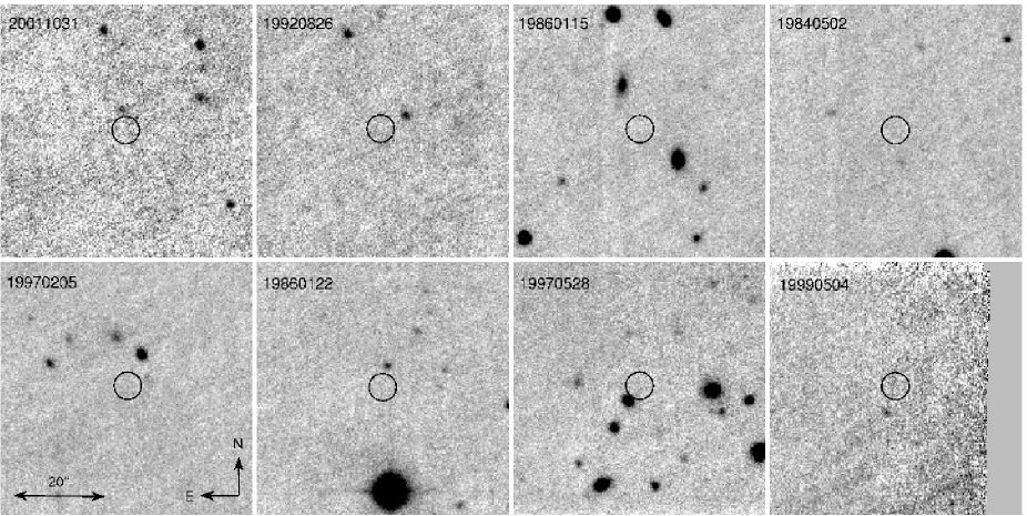
Figure 1.— P200/WIRC cutouts around the locations of the eight radio transients lacking optical counterparts found by Bower et al. (2007). The position of each transient is marked by a circle with $3^{\prime\prime}$ radius. The spatial radio position uncertainty of these transients is about $0.3^{\prime\prime}$ (Bower et al. 2007). The tie between the optical and radio coordinates frame is usually better than $1^{\prime\prime}$ (e.g. Gal-Yam et al. 2006). The transients names are noted at top-left of each cutout and are shown by their position East to West, upper row from left to right and than the lower row from left to right. The effective exposure times for the cutouts are: 1530 s, 3030 s, 7500 s, 7500 s, 7500 s, 5940 s, 4440 s, and 1530 s, respectively.

We do not detect any $K_{{\rm s}}$-band counterparts to each of these eight transients (see Table 1).

Also listed in Table 1 are the flux limits, at the position of the transients, from the ROSAT-PSPC all-sky survey in the 0.12–2.48 keV band (Voges et al. 1999).

4. Observational properties of the long-duration radio transients

In the following we analyze the observational properties of the long-duration radio transients. Specifically, we discuss their rate (§4.1), sky surface density (§4.2), and source count function (§4.3).

4.1. Rate

Bower et al. (2007) found that the observed areal density of events at 5 GHz and 8 GHz (dominated by the 5 GHz events), with flux density above 370 $\mu$Jy at a two-epoch survey, is $1.5\pm 0.4$ deg^-2. Thus, the single epoch areal density of events with flux greater than 370 $\mu$Jy, is $0.75_{-0.28,-0.45}^{+0.40,+0.81}$ deg^-2, where the errors are given at the 1- and 2-$\sigma$ confidence (using the formulation of Gehrels 1986). This is translated to a 5 GHz rate of events with flux density above $370\,\mu$Jy of

$$\Re_{5\,{\rm GHz},>0.37\,{\rm mJy}}=540_{-200,-330}^{+290,+590}\Big{(}\frac{t_{{\rm dur}}}{0.5\,{\rm day}}\Big{)}^{-1}\,{\rm deg}^{-2}\,{\rm yr}^{-1},$$ (1)

where $t_{{\rm dur}}$ is the (unknown) typical duration of these events and the errors are given at the 1- and 2-$\sigma$ confidence. $t_{{\rm dur}}$ can be a function of frequency. Therefore, comparison of this rate with rates at other frequencies should be treated with care. We are aware that our 5-GHz rate (Eq. 1) is much larger than the rate computed by Bower et al. (2007). However, the latter estimate was the result of an arithmetic error which once corrected yields the estimate given in Equation 1.

As can be gathered from Equation 1, the minimum rate is achieved for the largest value of $t_{{\rm dur}}$ which is seven days. Assuming a constant event rate, this minimum rate is $>9\times 10^{15}$ (at the $95\%$ confidence level [CL]) events over the Hubble time. For comparison, this estimate is several orders of magnitude larger than the population of any known Galactic class of sources. Therefore, if long-duration radio transients are Galactic, they must be repeaters. On the other hand, if the events are catastrophic (i.e., single-shot, not repeaters) then the mean time between events is $\mathrel{\raise 1.29167pt\hbox{$<$}\mkern-14.0mu\lower 2.58334pt\hbox{$\sim$}}100$ s (and possibly as small as $\sim 1$ s). The only known cosmological population with such high rate is supernovae ($\sim 1$ s^-1; see §5.1).

Next we look into the rates of these events in the 1.4-GHz band. As noted earlier (§2) the FIRST-NVSS analysis did not result in a firm detection of any long-duration transient. The total survey area of the FIRST-NVSS search, after correcting it for point-source incompleteness, source confusion due to the poor resolution of the NVSS and missing NVSS data, is 2500 deg² (see Levinson et al. 2002 for details). We place an upper limit to the sky density (i.e., density of sources observed in a single epoch) of transient sources (flux density above 6 mJy in the 1.4 GHz band) of $1.5\times 10^{-3}$ deg^-2 and $2.6\times 10^{-3}$ deg^-2, at the $95\%$ and $99.73\%$ CL, respectively. We note that this sky density is consistent with the upper limit derived by Carilli, Ivison & Frail (2003). Therefore, the $95\%$ confidence upper limit on the 1.4 GHz rate, $\Re$, of long duration radio transients with flux density above 6 mJy is:

$$\Re_{1.4\,{\rm GHz},>6\,{\rm mJy}}<1.1\Big{(}\frac{t_{{\rm dur}}}{0.5\,{\rm day}}\Big{)}^{-1}\,{\rm deg}^{-2}\,{\rm yr}^{-1}.$$ (2)

4.2. Sky Surface Density

Another interesting quantity is the areal density of the transients, $\Sigma$. We obtain a lower limit by dividing the number of unique sources by the angular area of the VLA field. All the Bower et al. transients were found within $9^{\prime}$ (twice the half-power radius at 5 GHz) from the center of a single VLA field ($\alpha=15^{h}02^{m}20.53^{s}$, $\delta=+78^{\circ}16^{\prime}14.905^{\prime\prime}$; J2000.0). Within the half-power radius of $4.5^{\prime}$ (corresponding to a solid angle of $0.018$ deg²) there are four detections (see Fig. 2 in Bower et al. 2007). At $95\%$ CL the smallest number of sources is $>1.1$ (using the formulation of Gehrels 1986). Therefore, at Galactic latitude $b\sim 40^{\circ}$, $\Sigma>60$ deg^-2 ($95\%$ CL).

We note that the lack of any repeater events in the Bower et al. (2007) sample can be used to improve this limit. This can be done by calculating the probability of choosing seven events out of $N$ with no repetition. However, the resulting areal density is only increased by 40% (to the same $95\%$ CL). We therefore retain the simpler estimate.

Assuming a constant surface density as a function of Galactic latitude the all-sky surface density of radio transient progenitors is $\Sigma_{{\rm all-sky}}>3.5\times 10^{6}$. We note that if the long duration radio transients are Galactic then their sky surface density toward the Galactic plane should be higher, and therefore the total all-sky number could be larger.

4.3. Source number count function

The source number count function, $N(>S)$, where $N$ is the number of events brighter than a peak flux density $S$, may provide some hints regarding the nature of the radio transient population. We consider a power-law source count function, $N(>S)\propto S^{n}$, where $n$ is the power-law index. For a homogeneous population of sources residing in an Euclidean Universe we expect $n=-3/2$, while for Galactic thin disk population $n\approx-1$.

Assuming that $t_{{\rm dur}}$ does not depend on the frequency, we can use the transient rates given in §4.1 to put limits on the power-law index, $n$, of the source number count function. For each expected value of the number of events detected in the Bower et al. (2007) survey, $\lambda_{b}$, and the Levinson et al. (2002) search, $\lambda_{l}$, we calculate the probability that $k_{b}=6$ events will be detected in the Bower et al. search and $k_{l}=0$ in the Levinson et al. survey:

$$P=\frac{1}{k_{l}!k_{b}!}\lambda_{b}^{k_{b}}e^{-\lambda_{b}}\lambda_{l}^{k_{l}}e^{-\lambda_{l}}.$$ (3)

The power-law index, $n$ relates to $\lambda_{b}/\lambda_{l}$ through:

$$\frac{\lambda_{b}}{\lambda_{l}}=\frac{A_{b}}{A_{l}}\Big{(}\frac{\nu_{b}}{\nu_{l}}\Big{)}^{n}\Big{(}\frac{S_{b}}{S_{l}}\Big{)}^{\alpha},$$ (4)

where $A_{b}=9.33$ deg² is the effective (single epoch) search area of the Bower et al. survey. This was estimated by dividing the number of transients found by Bower et al. (7), by the one epoch search areal density (0.75 deg^-2). $A_{l}=2500$ deg² is the area of the Levinson et al. search, $\nu_{b}=5$ GHz and $\nu_{l}=1.4$ GHz are the surveys frequencies, $S_{b}=0.37$ mJy and $S_{l}=6$ mJy are their specific flux limits, and $\alpha$ is the spectral power law index of the sources ($S_{\nu}\propto\nu^{\alpha}$). Equation 4 contains three parameters: $n$, $\lambda_{l}$ and $\lambda_{b}$. However $\lambda_{l}$ is a function of $n$ and $\lambda_{b}$. Thus we need only explore the phase space of two of these (e.g., $n$ and $\lambda_{b}$).

We calculated the probability in Equation 3 as a function of $n$ and $\lambda_{b}$. In Figure 2 we show the log likelihood contours as a function of $n$ and $\lambda_{b}$ for $\alpha=5/2$ and for $\alpha=0$. The contours are for the 1, 2 and 3-$\sigma$, assuming two degrees of freedom (Press et al. 1992).

For $\alpha=0$, we find $n<-1.8$ at the 3-$\sigma$ CL. Since such a steep number count index is unlikely for astrophysical sources, we conclude that most probably $\alpha\mathrel{\raise 1.29167pt\hbox{$>$}\mkern-14.0mu\lower 2.58334pt\hbox{$\sim$}}0$. The highest $\alpha$ possible for continuum emission is $\alpha=5/2$ (synchrotron self absorption; Rybicki & Lightman 1979, p. 186). For such $\alpha$ we find that $n<-0.7$ ($-1.0$) at the 3 (2)-$\sigma$ CL.

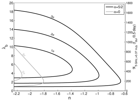
Figure 2.— Confidence interval contours (as calculated from the log-likelihood) as a function of the expected value of the number of events in the Bower et al. (2007) search, $\lambda_{b}$, and the power-law index $n$, of the source number count function (see Eq. 3). The gray lines show the 2- and 3-$\sigma$ contours for spectral index $\alpha=0$, while the black lines show the 1-, 2- and 3-$\sigma$ contours for $\alpha=5/2$. The right-hand y-axis is the corresponding transients rate assuming $t_{{\rm dur}}=0.5$ day.

There are at least two caveats in our analysis. First, we assumes that the source luminosity function does not depend on distance. Second, the Levinson et al. (2002) and Bower et al. (2007) rates were measured at different celestial positions. Therefore, if the long-duration radio transients are Galactic sources, then their sky distribution is probably not uniform, and this may affect the results presented in this section (however, see discussion in §6.1).

5. The progenitors of long-duration radio transients

In this section we list astrophysical sources and phenomenon that may be responsible for the long-duration radio transients. Some of these possibilities were already presented by Bower et al. (2007). We first discuss the extragalactic hypothesis (§5.1) followed by Galactic progenitors (§5.2).

5.1. Extragalactic sources

When observing the error boxes of known types of extragalactic explosions (e.g., GRBs and supernovae), we usually detect the host galaxy (e.g., Fruchter et al. 2006; Ovaldsen et al. 2007; Perley et al. 2009). In Figure 3 we present a histogram of the $R$-band magnitude (or limiting magnitude) for host galaxies of a sample of Swift (Gehrels et al. 2004) detected GRBs (Ovaldsen et al. 2007).

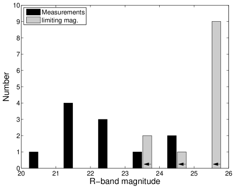
Figure 3.— $R$-band magnitude (black bars) or $2$-$\sigma$ limiting magnitude (gray bars) distribution of GRB host galaxies (Ovaldsen et al. 2007). In some cases the observations were done in a different band than $R$-band, in these cases, we converted the host galaxies magnitude to $R$-band by assuming it is an Sc-type galaxy at redshift of 2, based on the galaxy spectral templates of Kinney et al. (1996).

A high fraction ($\sim 50\%$) of the Swift GRBs are associated with galaxies brighter than about $R\sim 25$ mag. For optically identified supernovae (SNe) in blind surveys the fraction is almost $100\%$. We note that we still do not have deep images, and therefore constraints on the hosts, of the new class of bright supernovae (Barbary et al. 2009; Quimby et al. 2009).

We find it significant that only one of the Bower et al. transients has an optical counterpart (see §1). It is furthermore curious that this counterpart is a low redshift galaxy (RT 19840613; $z\cong 0.04$). Note the absence of any intermediate redshift counterparts.

Another way to quantify this curious absence of host galaxies is by using the observed star formation rate in the Universe. In Figure 4 we show the probability that the minimum redshift in a sample of seven sources randomly selected from the observed star formation rate distribution in the Universe (Hopkins & Beacom 2006) will be smaller than a given redshift. From Figure 4 we conclude that at least one of the seven radio transients will have $z<1.5$, at the $99.73\%$ CL. The luminosity function of galaxies at high redshift is not well known. However, the GRB host galaxies sample of Ovaldsen et al. (2007; Fig. 3) which probe typical redshifts of $\mathrel{\raise 1.29167pt\hbox{$>$}\mkern-14.0mu\lower 2.58334pt\hbox{$\sim$}}2$ suggest that if the radio transients residing in hosts similar to those of GRBs then Bower et al. should have detected optical counterparts to most of those transients.

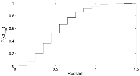
Figure 4.— The cumulative probability that the minimum redshift out of seven sources, randomly selected from the star formation distribution will be smaller than a given redshift. We used the star formation distribution compiled by Hopkins & Beacom (2006) using the parametrization of Cole et al. (2001) and assuming a modified Salpeter IMF. We divided this star formation distribution by $(1+z)$ to account for the decreasing transients rate due to time dilation.

The above discussion not withstanding we now consider the usual suspects in the extragalactic framework.

GRBs: Gamma-Ray Bursts (GRBs) are often detected in radio frequencies for periods of days to weeks (e.g., Frail et al. 1997; Chandra et al. 2008). However, as graphically demonstrated by Figure 3 the GRB hypothesis can be excluded. Furthermore, the observed all-sky rate of GRBs is $2$ day^-1, while the all-sky rate of long-duration radio transients is $\mathrel{\raise 1.29167pt\hbox{$>$}\mkern-14.0mu\lower 2.58334pt\hbox{$\sim$}}10^{3}$ day^-1 (§4.1).

Orphan GRBs: Observational evidences suggest that GRB emission is beamed and highly anisotropic (e.g., Harrison et al. 1999; Levinson et al. 2002). Therefore, the actual rate of orphan GRB explosions is $f_{b}^{-1}$ times larger than the observed rate. Here, $f_{b}^{-1}$ is the inverse of the beaming factor, and it is probably in the range 50–500 (e.g., Guetta, Piran & Waxman 2005; Gal-Yam et al. 2006). However, orphan GRB radio afterglows are expected to have time scales of years rather than days, which is not in line with the time scales of long-duration radio transients. More importantly, such orphans are expected to be at redshifts lower than that of GRBs (which are beamed and thus seen at higher redshift) making the host-galaxy non detections even more problematic (see Levinson et al. 2002).

Quasars and Active Galactic Nuclei: To a limiting magnitude of $i\approx 26$ mag, the faintest quasars can be detected to a redshift of about 5. The lack of optical counterparts associated with these transients is not consistent with a quasar connection. Low luminosity quasars (i.e., Active Galactic Nuclei; AGN), are fainter, but if their abundance roughly follows the star formation rate in the Universe, then as shown in Figure 4, the host galaxies should have been found in visible light.

Obscured quasars, also known as type-II quasars are faint in visible light frequencies. However, these sources may reveal themselves in near-IR (e.g., Gregg et al. 2002; Reyes et al. 2008). Figure 5 shows the $g$$-$$K$ and $R$$-$$K$ color of “normal” quasars as a function of redshift. The minimum $g$$-$$K$ color of quasars is about 2.5 mag. The non-detection of AGNs down to $K_{{\rm s}}$-band magnitude of 20.4 (§3) corresponds to a non detection of a quasar with intrinsic $g$-band magnitude fainter than $23$. This is based on the assumption that type-II quasars and normal quasars have similar $K$-band luminosity functions,

To this magnitude level, the faintest quasars can be detected up to $z\approx 2$. Therefore, the fact that we do not detect any near-IR sources associated with the long-duration radio transients disfavors association with reddened quasars.

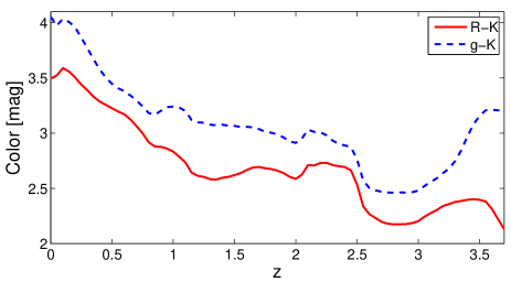
Figure 5.— The $R_{{\rm Vega}}$$-$$K_{{\rm Vega}}$ (solid line), and $g_{{\rm AB}}$$-$$K_{{\rm Vega}}$ (dashed line) colors, of quasars, as a function of redshift $z$. The colors are based on synthetic photometry of quasar spectral templates (Brotherton et al. 2001; Glikman, Helfand & White 2006). Synthetic photometry is calculated using the code of Poznanski et al. (2002). The minimum $g$$-$$K$ in the range $z=0$ to $z=3.7$ is about 2.5 mag. However, at $z>3.7$ the $g$$-$$K$ color will be larger since the Lyman $\alpha$ line is found at wavelength redder than that of the $g$-band.

Supernovae: There are two known variants of bright radio SNe: type-II radio SNe, for which SN 1979C (Weiler et al. 1991) is the prototype, and Type-Ic radio SN (e.g., SN 1998bw; Kulkarni et al. 1998).

Type-II radio SNe, have long time scales (years) and are detectable in nearby galaxies ($z\sim 0.01$). On the other hand, type-Ic radio SNe are detected to somewhat larger distances ($z\sim 0.1$), and last a few weeks. Therefore, based on the lack of optical counterparts we can rule out association with type-II or type-Ic radio SNe.

Extragalactic Microlensing: When considering microlensing events we should discuss the population of sources and lenses. While the lenses can be “unseen” objects, the sources should be radiant. Most sub-mJy sources, which are the potential sources for microlensing, are starburst galaxies. These galaxies have spatial size several orders of magnitude larger than the Einstein radius of stellar-mass lenses. Therefore, microlensing by extragalactic or Galactic objects cannot explain the high amplitude of the radio transients discussed here (Table 1).

We note that the small number of background sources and the high amplitude of the transients also rules out scintillation events.

Extragalactic Soft Gamma-Ray Repeaters (SGRs): There are only eight SGRs known in the Milky Way galaxy and the Magellanic Clouds. However, extragalactic SGRs (e.g., Eichler 2002; Nakar et al. 2006; Popov & Stern 2006; Ofek et al. 2006, 2008; Ofek 2007) may be detected to larger distances. Currently, the radio emission from giant flares of SGRs is not well constrained (see Cameron et al. 2005). Assuming a fraction of $10^{-4}$ of the energy released in hard X-rays/$\gamma$-rays is emitted in radio over one hour, a giant X-ray flare with luminosity $L_{X}\sim 10^{46}$ erg can be observed to a distance of a about 100 Mpc. However, the rate of SGR giant flares with such energy is about $10^{-4}-10^{-5}$ Mpc^-3 yr^-1 (Ofek 2007). Therefore, the expected observed rate of Galactic and extragalactic SGRs is at least three orders of magnitude smaller than the rate of long-duration radio transients.

New unknown explosions: Explosions taking place outside galaxies (“naked”) may explain the lack of optical counterparts. In general we can not rule out putative extra-Galactic sources, which have not been discovered yet.

We discuss several examples of such putative sources, showing that they are unlikely sources for the long-duration radio transients. Hawking (1974) suggested that primordial black holes of mass $\mathrel{\raise 1.29167pt\hbox{$<$}\mkern-14.0mu\lower 2.58334pt\hbox{$\sim$}}10^{15}$ g will evaporate within the Hubble time, and eventually emit a burst of energetic photons and particles. Such explosions are expected to manifest as a short-duration ($\ll 1$ s) radio pulse as the ambient magnetic field is altered by an expanding conducting shell (Rees 1977). However, to date such events were not found (e.g., Phinney & Taylor 1979). Moreover, they are expected to have very short time scales, in contrary to long-duration radio transients.

Following the suggestion by Kulkarni et al. (2009), Vachaspati (2008) presented a model in which grand unification scale superconducting cosmic strings are emitting short ($<1$ s) radio flares. Vachaspati (2008) predicts that the source number count function of such events will be $N(>S)\propto S^{-1/2}$, which is not consistent with the long-duration radio transients source count function (§4.3).

Strong radio emission from supernovae was suggested by Colgate & Noerdlinger (1971) and Colgate (1975). In their scenario, the expanding core of the supernova “combs” the star’s intrinsic dipole field, and the generated current sheet produce coherent radio emission. The maximum energy emitted in such a radio pulse, assuming no attenuation, is of the order of $10^{46}$ erg. However, the expected pulse is very short ($\ll 1$ s) in comparison to the observed time scale of long-duration radio transients. Of course, the lack of detectable host galaxies makes any such suggestion untenable.

The lack of optical counterparts cannot rule out association with high redshift sources (e.g., population-III stars). Assuming a large cosmological distance, the rest-frame energy of such events is approximately:

$$E_{f,cos} \approx 3\times 10^{48}\frac{S_{\nu}}{0.4\,{\rm mJy}}\frac{\Delta\nu}{10^{10}\,{\rm Hz}}\frac{t_{{\rm dur}}}{0.5\,{\rm day}}\Big{(}\frac{d_{L}}{5\times 10^{10}\,{\rm pc}}\Big{)}^{2}$$ (6)

$$\times\Big{(}\frac{1+z}{6}\Big{)}\,{\rm erg};$$

here, $d_{L}$ is the luminosity distance (normalized to $1+z=6$), $z$ is the redshift, and $S_{\nu}$, $\Delta{\nu}$, and $t_{{\rm dur}}$ are given in the observed frame.

The rest-frame brightness temperature (normalize at $1+z=6$) of such events is:

$$T_{{\rm B,cos}} = S_{\nu,{\rm rest}}d_{lum}^{2}(c/\nu_{{\rm rest}})^{2}(2\pi k_{B}R_{{\rm rest}}^{2})^{-1}$$ (7)

$$\approx 7\times 10^{16}\frac{S_{\nu}}{0.4\,{\rm mJy}}\Big{(}\frac{1+z}{6}\Big{)}^{-1}\Big{(}\frac{d_{L}}{5\times 10^{10}\,{\rm pc}}\Big{)}^{2}$$ (9)

$$\times\Big{(}\frac{\nu}{5\,{\rm GHz}}\Big{)}^{-2}\Big{(}\frac{R_{{\rm rest}}}{200\,{\rm au}}\Big{)}^{-2}\,{\rm K},$$

where we set the size of the emission region, $R_{{\rm rest}}$, to $200$ au which is the light crossing time in the rest frame, $ct_{{\rm dur,rest}}=ct_{{\rm dur}}(1+z)^{-1}$, for $t_{{\rm dur}}=7$ day. Again, $S_{\nu}$, $\Delta{\nu}$, and $t_{{\rm dur}}$ are given in the observer frame, while the subscript “rest” indicate quantities at the rest frame. As $t_{{\rm dur}}\mathrel{\raise 1.29167pt\hbox{$<$}\mkern-14.0mu\lower 2.58334pt\hbox{$\sim$}}7$ day, this is a lower limit on the brightness temperature. The huge brightness temperature, relative to the minimum energy or equipartition temperature (Readhead 1994), requires a coherent emission mechanism or alternatively a Lorentz factor of $\mathrel{\raise 1.29167pt\hbox{$>$}\mkern-14.0mu\lower 2.58334pt\hbox{$\sim$}}10^{2}$. However, if the beaming factor is large, then the rate of long-duration radio transients will exceed the SN rate in the Universe.

5.2. Galactic

Stellar sources: Several types of Galactic sources, which are known to flare at radio wavebands were discussed by Bower et al. (2007). Specifically, RS CVn stars, FK Com stars, Algol class binaries and X-ray binaries are ruled out by the lack of optical counterparts. Other possibilities, like T Tau stars, are associated with star forming regions typically found at low Galactic latitude.

Late-type stars are known to flare in radio wavebands (see Güdel 2002 for review). However, the lack of $R$- and $K$-band optical/near-IR counterparts rules out an association with late-type M-dwarfs up to a distance of 2 kpc, which is the median distance of Galactic M-dwarfs at the direction of the Bower et al. field (Gould, Bahcall, & Flynn 1996). Moreover, flares from M dwarfs (and brown dwarfs) are known to exhibit strong circular polarization ($\sim 100\%$; e.g., Hallinan et al. 2007; Berger 2006). However, as summarized in §1, Bower et al. (2007) did not find evidence for circular polarization above $30\%$ in any of their radio transients.

Brown dwarfs: In recent years, it was found that at least some brown-dwarfs are active, and show bursts in radio and X-ray wavebands (e.g., Burgasser et al. 2000; Berger et al. 2001; Berger et al. 2002; Burgasser & Putman 2005). In the radio regime, these flares peaks around 5 GHz (spectral slopes $\alpha\mathrel{\raise 1.29167pt\hbox{$>$}\mkern-14.0mu\lower 2.58334pt\hbox{$\sim$}}0$; Berger et al. 2001; 2005; 2008a;b).

Brown dwarfs are potentially very faint sources. Our near-IR search of the Bower et al. (2007) field can detect a T5-type brown dwarf up to distances of about 250 pc . However, our observations cannot rule out an association of the Bower et al. transients with older, or less massive, and hence cooler and fainter brown-dwarfs (e.g., Y-class brown-dwarfs; see Burrows et al. 1997; Baraffe et al. 2003 for evolutionary models).

For cooler brown-dwarfs which are undetectable by our $K$-band search, based on the minimum surface density of radio transient progenitors derived in §4.2, we can put a rough lower limit on the distance. We assume that the local density of brown dwarfs with effective temperature above 200 K is $\rho_{BD}\approx 0.1$ pc^-3 (Reid et al. 1999; Burgasser et al. 2004) and that at small distances the distribution can be regarded as isotropic. Agreement between the areal density of the radio transients (§4.2) to that of old brown dwarfs is obtained by having the brown dwarfs at a typical distance of $d\mathrel{\raise 1.29167pt\hbox{$>$}\mkern-14.0mu\lower 2.58334pt\hbox{$\sim$}}200$ pc.

At such distances, the energy needed to produce a single long-duration radio transient burst will be about:

$$E_{{\rm f,BD}} \approx 8\times 10^{30}\frac{S_{\nu}}{0.4\,{\rm mJy}}\Big{(}\frac{d}{200\,{\rm pc}}\Big{)}^{2}\frac{\Delta\nu}{10^{10}\,{\rm Hz}}$$ (11)

$$\times\frac{t_{{\rm dur}}}{0.5\,{\rm day}}\,{\rm erg}.$$

Should the Bower et al. radio transients arise from brown dwarfs then they must repeat. The flare repetition time scale is $\Sigma/\Re$. For the minimum sky surface density of $\Sigma\sim 60$ deg^-2 (§4.2), and assuming a rate $\Re\approx 500$ yr^-1 deg^-2, the repetition time scale is $\mathrel{\raise 1.29167pt\hbox{$>$}\mkern-14.0mu\lower 2.58334pt\hbox{$\sim$}}50$ day.

For a typical distance of 200 pc, the total energy emitted over the Hubble time from a single active Brown-dwarf will be $\sim 10^{42}$ erg. For comparison, the magnetic energy of active late-type M-dwarfs is:

$$E_{{\rm B}} = \frac{4}{3}\pi R_{*}^{3}\frac{B^{2}}{8\pi}$$ (12)

$$\cong 5.1\times 10^{35}\Big{(}\frac{r_{*}}{70000\,{\rm km}}\Big{)}^{3}\Big{(}\frac{B}{3\,{\rm kG}}\Big{)}^{2}{\rm erg},$$ (13)

where $R_{*}$ is the star radius, and $B$ is its magnetic field. We note that magnetic fields in the most magnetically active M-dwarfs reach several kG (e.g., Valenti, Marcy, & Basri 1995; Johns-Krull & Valenti 1996; Berger et al. 2008b). This is several orders of magnitude smaller than the total energy output of a long-duration radio transient. Therefore, this scenario requires that the magnetic field of brown-dwarfs will be replenished from an internal energy source. This is not an implausible suggestion. For example, $10^{42}$ erg is only a small fraction of the brown dwarf thermal or rotational energy. The strongest argument against the association of long-duration radio transients with brown dwarfs is the lack of circular polarization observed in the Bower et al. (2007) events.

Reflected solar flares: As discussed by Bower et al. (2007), a solar flare reflected by a solar system object will have a flux of:

$$S_{{\rm ref}} = 6.6\frac{S_{\odot,flare}}{10^{8}\,{\rm Jy}}\frac{A}{0.6}\Big{(}\frac{d}{100\,{\rm km}}\Big{)}^{2}$$ (15)

$$\times\Big{(}\frac{r}{1\,{\rm au}}\Big{)}^{-2}\Big{(}\frac{\Delta}{1\,{\rm au}}\Big{)}^{-2}\,\mu{\rm Jy},$$

where $S_{\odot,flare}$ is the solar flare flux density, $r$ and $\Delta$ are the distance of the asteroid from the Sun and Earth, respectively, and $A$ is its albedo. Strong X-class solar flares may have flux densities of $10^{8}$ Jy, although they typically last less than 20 minute (Bastian, Benz, & Gary 1998). Moreover, in order to explain the long-duration radio transients using such reflected events, we need a population of huge asteroids ($d>100$ km), at near Earth orbits, which do not exist. More importantly, the motion of such objects will be detectable by the VLA in A array whereas the Bower et al. transients are point sources.

Pulsars: Most of the Galactic pulsars are young objects (up to $10^{8}$ yr), and found near the Galactic plane. Moreover, with the exception of magnetars, known pulsars have radio spectrum with $\alpha\approx-2$ (e.g., Camilo et al. 2006). Based on the catalogue of simulated NSs (Ofek 2009), the expected surface density of NSs with age smaller than 10 (100) Myr, at the direction of the Bower et al. field, is about 0.3 (8) deg^-2, assuming $10^{9}$ NSs in the Galaxy. We note that the number of NSs in the direction of the Bower et al. field ($b\cong 37^{\circ}$) rises faster than linearly with age, since NSs are born in the Galactic plane and ejected (mostly) to high Galactic latitudes.

Isolated old neutron stars: The Galaxy may host about $10^{9}$ old isolated NSs (see §6.1). This is a plausible hypothesis and we discuss this in the next section.

To conclude, the analysis of Bower et al. (2007) and our own analysis does not favor association of the long-duration radio transients with many types of astrophysical sources. However, we cannot rule out association of the long-duration radio transients with Galactic isolated NSs, Galactic cool brown-dwarfs, or some sort of exotic explosion. Although cool brown dwarfs are interesting candidates, they require an emission mechanism which does not produce circularly polarized radiation like that observed in flare stars.

6. Isolated-old neutron stars as progenitors of the long-duration radio transients

The organization of this section is as follows. In §6.1 we give a brief introduction to old neutron stars. Based on Monte-Carlo orbital simulations of NSs we estimate their sky surface density, distances and source number counts function (§6.2). In §6.3 we discuss the energetics of long-duration radio transients in the context of Galactic NS. In §6.4 we present a simple synchrotron emission model for such radio flares, while in §6.5 we discuss the possibility that these are some kind of intermittent pulsars. Finally, we derive a lower and upper limits on the distance scale to the Kida et al. transients assuming they are originating from Galactic NSs (§6.6).

6.1. Introduction to Galactic isolated old NS

Based on the metal content of the Milky Way galaxy, Arnett, Schramm & Truran (1989) estimated that about $10^{9}$ SNe exploded in the Milky Way and hence similar number of NSs were born in our Galaxy. The observed SN rate in the Galaxy suggests a number which is smaller by a factor of 3–10. Thus it is expected that there are about $10^{8}$ to $10^{9}$ NS in the Galaxy.

NSs cool on relatively short time scales ($\sim$$10^{6}$ yr; e.g., Yakovlev & Pethick 2004). Therefore, they are expected to be intrinsically dim and extremely hard to detect. However, Ostriker et al. (1970) suggested that NSs may be heated through accretion of inter-stellar matter (ISM). This novel suggestion raised many hopes that NSs may be detected as soft X-ray sources (e.g., Helfand, Chanan & Novick 1980; Treves & Colpi 1991; Blaes & Madau 1993). These predictions were followed by intensive searches for such objects (e.g., Motch et al. 1997; Maoz, Ofek, & Shemi 1997; Haberl, Motch, & Pietsch 1998; Rutledge et al. 2003; Agüeros et al. 2006). However, the several candidates that were found (e.g., Haberl, Motch, & Pietsch 1998) are young cooling NSs (e.g., Neuhäuser & Trümper 1999; Popov et al. 2000; Treves et al. 2001).

Among the usual explanations for the observational paucity of isolated accreting old NSs in the ROSAT all-sky survey (Voges et al. 1999) are the fact that the velocity distribution of NSs is much higher than the early estimates (e.g., Narayan & Ostriker [1990] vs. Cordes & Chernoff [1998]) or the suggestion that magnetized NSs cannot accrete matter efficiently at the Bondi-Hoyle rate (e.g., Colpi et al. 1998; Perna et al. 2003).

6.2. Surface density and distance

In order to estimate the surface density we need a model for isolated old NS space distribution at the current epoch. Ofek (2009) integrated the orbits of simulated NSs in the Galactic gravitational potential, using two different natal velocity distributions and vertical scale height distributions of the progenitor populations suggested by Arzoumanian et al. (2002) and Faucher-Giguère & Kaspi (2006). These simulations assume that $60\%$ of the Galactic NSs were born in the Galactic bulge 12 Gyr ago, while $40\%$ were born continuously, with a constant rate, in the disk over the past 12 Gyr.

Based on this catalog, and using the Arzoumanian et al. initial conditions, in Figure 6 we show the theoretical sky surface density of all Galactic NSs, and NSs within 1 kpc from the Sun.

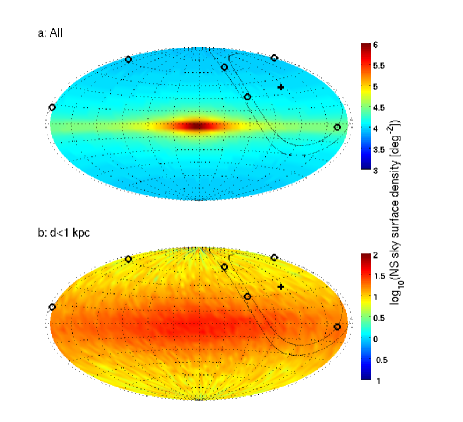
Figure 6.— Sky surface density distribution of all NSs (panel a) and NSs at distance $<1$ kpc from the Sun (panel b). The maps are presented in the Galactic coordinate system and using the Aitoff equal area projection. The sky surface density are calculated using the catalog of simulated old NSs presented in Ofek (2009) including both populations of bulge-born and disk-born NSs, and using the natal velocity distribution of Arzoumanian et al. (2002) and assuming $10^{9}$ NSs. The plus sign marks the position of the Bower et al. (2007) field at $l=115^{\circ}$, $b=37^{\circ}$. The lines mark the declination zone of 32^∘ to 42^∘, in which the survey for radio transients described by Kida et al. (2008) was conducted. The six circles mark the position of the bright (flux at 1.4 GHz greater than $1$ Jy) transients reported by Kida et al. (2008).

Towards the direction of the Bower et al. (2007) field, the total surface density of isolated old NSs is about $10^{4}$ deg^-2. The mean surface density of old NSs at Galactic latitude $b>30^{\circ}$, which roughly corresponds to the FIRST survey footprint, is about $5\%$ larger. The small difference between the two surface densities suggests that if indeed long-duration radio transients are associated with isolated old NSs then the comparison between the 1.4 GHz and 5 GHz rates presented in §4.3 is not affected by the different sky positions at which these surveys were conducted.

In Figure 7 we show the cumulative surface density of NSs, at the Bower et al. (2007) field direction, as a function of distance from the observer (i.e., the Sun). The plots assume that the Sun is located 8 kpc from the Galactic center (Ghez et al. 2008). In Figure 7 we also mark, by a dotted horizontal line, the minimal sky surface density of long-duration radio transients (i.e., $\Sigma>60$ deg^-2) that we derived in §4.2. This Figure suggests that if isolated old NSs are indeed related to the sub-mJy level Bower et al. transients then their typical distance scale is at least $\sim 1$ kpc. Otherwise the predicted sky surface density will not be consistent with the minimum sky surface density of NS at the direction of the Bower et al. field (see §4.2). On the other hand, the typical distance is presumably not greater than about 5 kpc, otherwise the slope of the cumulative distribution will be too shallow relative to the steep power-law index, $n$, of the number count distribution derived in §4.3. We note that the luminosity function of these hypothetical events may depend on the age (and therefore distance) to the NSs. Therefore, we do not attempt to quantify the upper limit on the distance mentioned above.

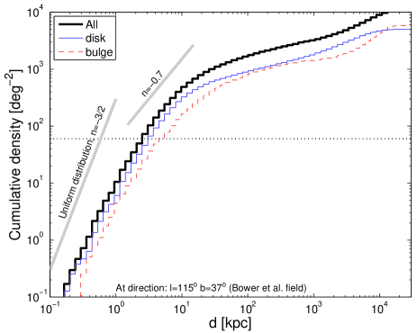
Figure 7.— Cumulative number of simulated NSs per deg² at the direction of the Bower et al. (2007) field as a function of distance. The thick solid line shows the distribution of the entire NS population of which $60\%$ ($40\%$) are assumed to be of bulge (disk) origin, the thin solid line is for the disk-born NSs, while the dashed line is for the bulge-born NSs. The three distributions give a rough idea regarding the uncertainties that may arise from our ignorance regarding the birth locations of NSs along Galactic history. The dotted horizontal line marks the minimum surface density required ($60$ deg^-2; see §4.2). The thick solid gray lines show the expected slopes for a population with a homogeneous distribution ($n=-3/2$), and $n=-0.7$, which corresponds to our $3$-$\sigma$ upper limit (see however text).

A possibility that we should consider is that only a fraction of the Galactic NSs are the progenitors of the long-duration radio transients (e.g., only “young” NSs). Based on the NSs orbital simulations, we find that all the NSs with ages smaller than at least 1 Gyr are required as progenitors of the radio transients. Thus, the sub-mJy long duration radio transients cannot arise from pulsars.

A simple test for the hypothesis that long-duration radio transients are associated with Galactic isolated old NSs (or for that matter any Galactic population with radial scale length of a kpc or so) is to look for excess of sub-mJy radio transients near the Galactic center, relative to high Galactic latitude. In Figure 8 we therefore show the cumulative distribution of isolated old NSs as a function of distance, but towards the direction of the Galactic center.

There are several marked differences between Figures 7 and 8. The total sky surface density in the direction of the Galactic center is about two orders of magnitude larger than the sky surface density at the direction of the Bower et al. field. Next, if we consider only NSs with distances up to 1 kpc, then the sky surface density in the direction of the Galactic center is about seven times larger than that in the Bower et al. field. Finally, the source count function in the direction of the Galactic center is steeper than that in the direction of the Bower et al. (2007) field.

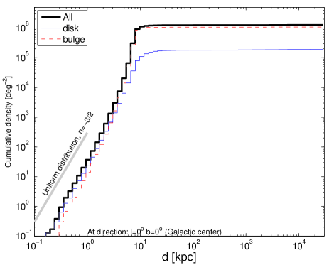
Figure 8.— Like Fig. 7, but towards the direction of the Galactic center.

6.3. Energetics and time scales

In the old-NS framework the typical energy release from a single flare is:

$$E_{{\rm f}} \approx 2\times 10^{32}\frac{S_{\nu}}{0.4\,{\rm mJy}}\Big{(}\frac{d}{1\,{\rm kpc}}\Big{)}^{2}$$ (17)

$$\times\frac{\Delta\nu}{10^{10}\,{\rm Hz}}\frac{t_{{\rm dur}}}{0.5\,{\rm day}}\,{\rm erg}.$$

The rate of the sub-mJy long-duration radio transients is in the range of $\Re\approx 20$ deg^-2 yr^-1 to $2\times 10^{4}$ deg^-2 yr^-1 (Eq. 1). Adopting a representative rate of $\Re\approx 500$ deg^-2 yr^-1, and $t_{{\rm dur}}\sim 0.5$ day we find that over the Hubble time the all-sky number of events is larger by several orders of magnitude than that of any known Galactic stellar population. Therefore, any hypothesis involving Galactic stars would require that the sources be repeaters. The mean time scale between bursts, $\Delta{t_{{\rm b}}}$, is given by:

$$\Delta{t_{{\rm b}}} = \frac{\Sigma}{\Re}$$ (18)

$$\cong 0.2\frac{\Sigma}{10^{2}\,{\rm deg}^{-2}}\Big{(}\frac{\Re}{500}\Big{)}^{-1}\,{\rm yr}$$ (19)

$$\cong 0.2\frac{\Sigma}{10^{2}\,{\rm deg}^{-2}}\frac{t_{{\rm dur}}}{0.5\,{\rm day}}\,{\rm yr},$$ (20)

where $\Sigma$ is the sky surface density of sources in the direction of the Bower et al. (2007) field. In that case the flares duty cycle is of order of $\mathcal{D}=t_{{\rm dur}}/\Delta{t_{b}}\approx 7\times 10^{-3}$. An immediate prediction is that if long-duration radio transients are associated with Galactic NSs, then the repetition time scale for bursts is relatively short, of the order of several months.

Multiplying Equation 17 by the expected number of flares within the Hubble time ($t_{{\rm H}}/\Delta{t}_{{\rm b}}\sim 5\times 10^{10}$, where $t_{{\rm H}}$ is the Hubble time), we find that the total energy emitted by a single object over its life time is:

$$E_{{\rm tot}} \approx 1\times 10^{43}\frac{S_{\nu}}{0.4\,{\rm mJy}}\Big{(}\frac{d}{1\,{\rm kpc}}\Big{)}^{2}\frac{\Delta\nu}{10^{10}\,{\rm Hz}}$$ (22)

$$\times\Big{(}\frac{\Sigma}{10^{2}\,{\rm deg}^{-2}}\Big{)}^{-1}\,{\rm erg},$$

Dividing Equation 17 by Equation 20, the mean luminosity over time required in order to power these bursts is:

$$\langle\dot{E}\rangle \approx 3\times 10^{25}\frac{S_{\nu}}{0.4{\rm mJy}}\Big{(}\frac{d}{1\,{\rm kpc}}\Big{)}^{2}\frac{\Delta\nu}{10^{10}\,{\rm Hz}}$$ (24)

$$\times\Big{(}\frac{\Sigma}{10^{2}\,{\rm deg}^{-2}}\Big{)}^{-1}\,{\rm erg\,s}^{-1}.$$

Note that this quantity is independent of $\Delta t_{{\rm b}}$.

Next, we consider the energy reservoir of isolated old NSs, and check whether it is consistent with the mean luminosity given by Equation 24. Isolated old NSs have several sources of available energy. Among these are: (i) spin energy; (ii) magnetic energy; and (iii) accretion, from the ISM, energy.

The rotational kinetic energy of NSs is:

$$E_{{\rm rot}} = \frac{1}{2}I\omega^{2}$$ (25)

$$\cong 2.2\times 10^{44}\Big{(}\frac{P}{10\,{\rm s}}\Big{)}^{-2}\frac{M_{{\rm NS}}}{1.4\,{\rm M}_{\odot}}\Big{(}\frac{R_{{\rm NS}}}{10\,{\rm km}}\Big{)}^{2}\,{\rm erg},$$ (26)

where $M_{{\rm NS}}$ is the NS mass, $I$ is the moment of inertia (assuming $I=0.4M_{{\rm NS}}R_{{\rm NS}}^{2}$), $\omega$ is the NS rotational angular speed, and $P$ ($=2\pi/\omega$) is its rotation period. The energy-loss rate available from the rotational energy reservoir is:

$$\dot{E}_{\rm rot} = I\omega\dot{\omega}=4\pi^{2}IP^{-3}\dot{P}$$ (27)

$$\cong 4.4\times 10^{26}\frac{M_{{\rm NS}}}{1.4\,{\rm M}_{\odot}}\Big{(}\frac{R_{{\rm NS}}}{10\,{\rm km}}\Big{)}^{2}$$ (29)

$$\times\Big{(}\frac{P}{10\,{\rm s}}\Big{)}^{-3}\frac{\dot{P}}{10^{-17}}\,{\rm erg\,s}^{-1},$$

where $\dot{\omega}$ is the time derivative of the NS angular frequency, and $\dot{P}$ is defined as minus of its period derivative. Typical values for $\dot{P}$ are in the range of $10^{-10}$ s ṡ for magnetars, $10^{-17}$ s ṡ to $10^{-12}$ s ṡ for normal radio pulsars, and $10^{-21}$ s ṡ to $10^{-18}$ s ṡ for millisecond pulsars (Srinivasan 1989).

A large fraction of NSs may have high surface magnetic field in excess of $10^{14}$ G (e.g., Magnetars). The energy stored in the magnetic field of such objects is about:

$$E_{{\rm B}} \approx \frac{4}{3}\pi R_{{\rm NS}}^{3}\frac{B^{2}}{8\pi}$$ (30)

$$\approx 1.7\times 10^{45}\Big{(}\frac{r_{{\rm NS}}}{10\,{\rm km}}\Big{)}^{3}\Big{(}\frac{B}{10^{14}\,{\rm G}}\Big{)}^{2}{\rm erg},$$ (31)

where $R_{{\rm NS}}$ is the NS radius, and $B$ is its interior mean magnetic field. We note that the internal magnetic field may be higher, and therefore, Equation 31 is a lower limit on the magnetic energy reservoir. The rate at which the magnetic field of NSs is decaying is debated both theoretically and observationally (e.g., Urpin & Muslimov 1992; Chanmugam 1992; Phinney & Kulkarni 1994; Sengupta 1997; Sun & Han 2002). Assuming the magnetic field is uniformly decaying on the Hubble time scale, this will provide, on average, energy loss rate of $\dot{E}\approx 4\times 10^{27}$ erg s^-1.

Another possible source of energy is heating of the NS by accretion from the ISM (e.g., Ostriker et al. 1970). Assuming NSs accrete at the Bondi-Hoyle rate (Bondi & Hoyle 1944), the energy-loss rate will be:

$$\dot{E}_{{\rm acc}} = \frac{4\pi G^{3}M_{{\rm NS}}^{3}\rho_{{\rm ISM}}}{R_{{\rm NS}}(v^{2}+c_{s}^{2})^{3/2}}$$ (32)

$$\approx 5\times 10^{26}\Big{(}\frac{M_{{\rm NS}}}{1.4\,{\rm M}_{\odot}}\Big{)}^{3}\Big{(}\frac{R_{{\rm NS}}}{10\,{\rm km}}\Big{)}^{-1}$$ (34)

$$\times\frac{n_{{\rm ISM}}}{0.1{\rm cm}^{-3}}\Big{(}\frac{v}{300\,{\rm km\,s}^{-1}}\Big{)}^{-3}\,{\rm erg}\,{\rm s}^{-1},$$

where $v$ is the velocity of the NS relative to an ISM with a mass (number) density $\rho_{{\rm ISM}}$ ($n_{{\rm ISM}}$). $c_{s}$ is the sound speed in the ISM, which is of the order of 10 km s^-1 and is therefore neglected. We note, however, that magneto hydrodynamic simulations suggest that in the presence of a strong magnetic field the accretion rate will be suppressed relative to the Bondi rate (e.g., Toropina et al. 2001, 2003, 2005; see however Arons & Lea 1976, 1980).

To conclude, the combination of NSs energy sources may provide enough energy to explain long-duration radio transients. Specifically, the rotation energy of NSs and the energy available for NSs from accretion from the ISM is at least an order of magnitude larger than needed for generating the long-duration radio transients (Eq. 24). However, unless additional energy sources are invoked, this implies that the outbursts can not emit much higher energy at other frequencies.

6.4. Incoherent synchrotron radiation from an afterglow

Now we address the mechanism of radio emission. There are two possibilities: (i) incoherent synchrotron emission (the afterglow model); and (ii) coherent emission. We discuss the first possibility in this section and the second possibility in §6.5.

In the afterglow model, the source undergoes an explosive event and ejects relativistic particles and may generate magnetic field (hereafter relativistic plasma). Some sort of pressure confinement is needed to prevent rapid expansion of the relativistic plasma. Otherwise the expansion or adiabatic losses vastly increase the energy budget which would be inconsistent with the old NS framework. In the case of GRBs, the afterglow is confined by the dynamic pressure of the blast wave. We return to this critical issue towards the end of the subsection. We proceed by computing the (quasi)static properties of the (approximately) confined relativistic plasma. We note that the parameters derived from this model are estimated to within an order of magnitude.

Our simple model involves four free parameters: the radius of the emitting region, $R$; the mean electron density, $n_{{\rm e}}$; the magnetic field, $B$; and the characteristic electron Lorentz factor, $\gamma_{{\rm e}}=(1-\beta_{{\rm e}}^{2})^{-1/2}$, where $\beta_{{\rm e}}$ is the typical electron speed in units of the speed of light. The large value of the 5 GHz rate (Eq. 1) relative to that at 1.4 GHz rate (Eq. 2) suggests that the synchrotron self absorption frequency is above 5 GHz (see §4.3). Therefore, we assume $\nu_{s}\mathrel{\raise 1.29167pt\hbox{$>$}\mkern-14.0mu\lower 2.58334pt\hbox{$\sim$}}5$ GHz, and that the optical depth at 5 GHz, $\tau_{5}>1$. Furthermore, we assume that the optical depth at the synchrotron frequency $\tau_{s}\mathrel{\raise 1.29167pt\hbox{$<$}\mkern-14.0mu\lower 2.58334pt\hbox{$\sim$}}1$.

In order to estimate these parameters, we use the following relations:

(i) The characteristic synchrotron frequency:

$$\nu_{s} = \gamma_{{\rm e}}^{2}\frac{eB}{2\pi m_{{\rm e}}c}$$ (35)

$$\cong 2.8\times 10^{6}\gamma_{{\rm e}}^{2}B\,{\rm Hz},$$ (36)

where $e$ is the elementary (electron) charge, $m_{{\rm e}}$ is the electron mass, and $B$ the magnetic field in cgs units (i.e., Gauss).

(ii) The power emitted by a relativistic single electron due to synchrotron radiation (e.g., Rybicki & Lightman 1979) is:

$$P_{s} = \frac{4}{3}\sigma_{T}c\beta^{2}\gamma_{{\rm e}}^{2}U_{B}$$ (37)

$$\cong 1.1\times 10^{-15}\beta^{2}\gamma_{{\rm e}}^{2}B^{2}\,{\rm erg}\,{\rm s}^{-1},$$ (38)

where $\sigma_{T}$ is the Thomson cross-section, and $U_{B}=B^{2}/(8\pi)$ is the magnetic field energy density. The synchrotron cooling time scale, assuming $\tau_{s}\mathrel{\raise 1.29167pt\hbox{$<$}\mkern-14.0mu\lower 2.58334pt\hbox{$\sim$}}1$, is given by

$$t_{{\rm syn}} = \frac{\gamma_{{\rm e}}m_{{\rm e}}c^{2}}{P_{{\rm s}}}$$ (39)

$$\cong 7.7\times 10^{8}\gamma_{{\rm e}}^{-1}\beta^{-2}B^{-2}\,{\rm s}.$$ (40)

(iii) The brightness temperature, $T_{{\rm B}}$ (essentially a conveniently chosen surrogate for distance) is:

$$T_{{\rm B}} = S_{\nu}d^{2}(c/\nu)^{2}(2\pi k_{{\rm B}}R^{2})^{-1}$$ (41)

$$\cong 1.6\times 10^{21}\frac{S_{\nu}}{0.4\,{\rm mJy}}\Big{(}\frac{d}{1\,{\rm kpc}}\Big{)}^{2}$$ (43)

$$\times\Big{(}\frac{\nu}{5\,{\rm GHz}}\Big{)}^{-2}\Big{(}\frac{R}{10\,{\rm km}}\Big{)}^{-2}\,{\rm K},$$

where $\nu$ is the frequency at which we observe (i.e., 5 GHz). For optical depth larger than unity the brightness temperature is related to the electrons energy:

$$k_{{\rm B}}T_{{\rm B}}\approx\gamma_{{\rm e}}m_{{\rm e}}c^{2}.$$ (44)

(iv) Finally, in order to get a self absorption spectrum (see §4.3) the optical depth at 5 GHz should be larger than unity. This holds if and only if at 5 GHz the thermal emission is smaller than the optically thin emission:

$$2\pi k_{{\rm B}}T_{{\rm B}}\Big{(}\frac{\nu}{c}\Big{)}^{2}<\frac{1}{3}Rn_{{\rm e}}\frac{P_{{\rm s}}}{\nu_{{\rm s}}}\Big{(}\frac{\nu}{\nu_{{\rm s}}}\Big{)}^{1/3}$$ (45)

Next, we can solve equations 36–45 for the free parameters $B$, $\gamma_{{\rm e}}$, and $R$ and we can put a lower limit on the value of $n_{{\rm e}}$. Since we do not know the exact value of $t_{{\rm dur}}$, $\nu_{{\rm s}}$ and $d$ we solve for the free parameters as a function of these arguments. For completeness, we also state the dependency on $S_{\nu}$. We normalized the solutions for $S_{\nu}=0.4$ mJy, $d=1$ kpc, $t_{{\rm syn}}\approx t_{{\rm dur}}=0.5$ day, and $\nu_{{\rm s}}=2\times 10^{11}$ Hz (the choice for $\nu_{{\rm s}}$ is to minimize the total energy; see below). We note that $t_{{\rm dur}}\approx t_{{\rm syn}}$ means that there is no energy injection into the emission region after the initial burst (i.e., the duration of the events is dominated by the synchrotron cooling time scale). However, if energy is injected then $t_{{\rm dur}}\mathrel{\raise 1.29167pt\hbox{$>$}\mkern-14.0mu\lower 2.58334pt\hbox{$\sim$}}t_{{\rm syn}}$.

The following solution holds for $\tau_{5}\mathrel{\raise 1.29167pt\hbox{$>$}\mkern-14.0mu\lower 2.58334pt\hbox{$\sim$}}1$ and $\tau_{{\rm s}}\mathrel{\raise 1.29167pt\hbox{$<$}\mkern-14.0mu\lower 2.58334pt\hbox{$\sim$}}1$:

$$B\approx 17\Big{(}\frac{\nu_{{\rm s}}}{2\times 10^{11}\,{\rm Hz}}\Big{)}^{-1/3}\Big{(}\frac{t_{{\rm syn}}}{0.5\,{\rm day}}\Big{)}^{-2/3}\,{\rm G},$$ (46)

$$\gamma_{{\rm e}}\approx 66\Big{(}\frac{\nu_{{\rm s}}}{2\times 10^{11}\,{\rm Hz}}\Big{)}^{2/3}\Big{(}\frac{t_{{\rm syn}}}{0.5\,{\rm day}}\Big{)}^{1/3},$$ (47)

$$R \approx 6\times 10^{10}\Big{(}\frac{\nu_{{\rm s}}}{2\times 10^{11}\,{\rm Hz}}\Big{)}^{-1/3}\Big{(}\frac{t_{{\rm syn}}}{0.5\,{\rm day}}\Big{)}^{-1/6}$$ (49)

$$\times\Big{(}\frac{S_{\nu}}{0.4\,{\rm mJy}}\Big{)}^{1/2}\Big{(}\frac{d}{1\,{\rm kpc}}\Big{)}\,{\rm cm},$$

and the lower limit on $Rn_{{\rm e}}$ is

$$Rn_{{\rm e}}>2\times 10^{16}\Big{(}\frac{\nu_{{\rm s}}}{2\times 10^{11}\,{\rm Hz}}\Big{)}^{4/3}\frac{t_{{\rm syn}}}{0.5\,{\rm day}}\,{\rm cm}^{-2}.$$ (50)

We note that in order to minimize the energy, $n_{{\rm e}}$ should be around the lower limit implied by Equation 50. For convenient we also give the brightness temperature:

$$T_{{\rm B}} \approx 4\times 10^{11}\Big{(}\frac{\nu_{{\rm s}}}{2\times 10^{11}\,{\rm Hz}}\Big{)}^{2/3}$$ (52)

$$\times\Big{(}\frac{t_{{\rm syn}}}{0.5\,{\rm day}}\Big{)}^{1/3}\,{\rm K}.$$

Next, we can derive the ratio between the magnetic energy and electron energy densities:

$$U_{{\rm B}}/U_{{\rm e}} = \frac{B^{2}/(8\pi)}{n_{{\rm e}}\gamma_{{\rm e}}m_{{\rm e}}c^{2}}$$ (53)

$$\mathrel{\raise 1.29167pt\hbox{$<$}\mkern-14.0mu\lower 2.58334pt\hbox{$\sim$}} 1\Big{(}\frac{\nu_{{\rm s}}}{2\times 10^{11}\,{\rm Hz}}\Big{)}^{-3}\Big{(}\frac{t_{{\rm syn}}}{0.5\,{\rm day}}\Big{)}^{-17/6}$$ (55)

$$\times\Big{(}\frac{S_{\nu}}{0.4\,{\rm mJy}}\Big{)}^{1/2}\Big{(}\frac{d}{1\,{\rm kpc}}\Big{)},$$

where $U_{{\rm e}}=n_{{\rm e}}\gamma_{{\rm e}}m_{{\rm e}}c^{2}$ is the electrons energy density. We note that $U_{{\rm B}}/U_{{\rm e}}$ is very sensitive to both the duration, $t_{{\rm syn}}$, and the synchrotron frequency, $\nu_{{\rm s}}$, whose values are not well known. Therefore, a small change in these unknown parameters will change $U_{{\rm B}}/U_{{\rm e}}$ dramatically (see also Readhead 1994).

We note that by setting $U_{{\rm B}}/U_{{\rm e}}\sim 1$, we have ensured that $T_{{\rm B}}$ is equal to the equipartition brightness temperature (Readhead 1994) and minimized the energy requirement. Next we test if these parameters are below the inverse-Compton catastrophe limit (Kellermann & Pauliny-Toth 1969). The inverse-Compton catastrophe is relevant if $U_{{\rm rad}}/U_{{\rm B}}\mathrel{\raise 1.29167pt\hbox{$>$}\mkern-14.0mu\lower 2.58334pt\hbox{$\sim$}}1$. Assuming $\tau_{{\rm s}}\mathrel{\raise 1.29167pt\hbox{$<$}\mkern-14.0mu\lower 2.58334pt\hbox{$\sim$}}1$:

$$U_{{\rm rad}}\approx\frac{RU_{{\rm e}}}{ct_{{\rm syn}}}.$$ (56)

Since $R/(ct_{{\rm syn}})\ll 1$ we get $U_{{\rm rad}}\ll U_{{\rm e}}\sim U_{{\rm B}}$. Therefore, inverse-Compton effects can be neglected.

Assuming the electron density is close to the minimum density implied by Equation 50, the total energy in a single burst (i.e., in both the electrons and magnetic field) is given by:

$$E = \frac{4}{3}\pi R^{3}(U_{{\rm e}}+U_{{\rm B}})$$ (57)

$$\cong 1\times 10^{34}\Big{[}\Big{(}\frac{\nu_{{\rm s}}}{2\times 10^{11}\,{\rm Hz}}\Big{)}^{4/3}\Big{(}\frac{t_{{\rm syn}}}{0.5\,{\rm day}}\Big{)}$$ (61)

$$\times\Big{(}\frac{S_{\nu}}{0.4\,{\rm mJy}}\Big{)}\Big{(}\frac{d}{1\,{\rm kpc}}\Big{)}^{2}\Big{]}$$

$$+1\times 10^{34}\Big{[}\Big{(}\frac{\nu_{{\rm s}}}{2\times 10^{11}\,{\rm Hz}}\Big{)}^{-5/3}\Big{(}\frac{t_{{\rm syn}}}{0.5\,{\rm day}}\Big{)}^{-11/6}$$

$$\times\Big{(}\frac{S_{\nu}}{0.4\,{\rm mJy}}\Big{)}^{3/2}\Big{(}\frac{d}{1\,{\rm kpc}}\Big{)}^{3}\Big{]}\,{\rm erg}.$$

The specific values we have selected, $\nu_{{\rm s}}=2\times 10^{11}$ Hz and $t_{{\rm syn}}=0.5$ day, give a solution which is near equipartition and therefore minimizes the energy. For $n_{{\rm e}}$ close to its minimum implied by Equation 50, the total energy in a burst, and $U_{{\rm B}}/U_{{\rm e}}$ as a function of $\nu_{{\rm s}}$ and $t_{{\rm syn}}$ are shown in Figure 9. This Figure suggests that the minimum energy required per burst is around $10^{34}$ erg. This energy per burst multiplied by the expected number of bursts over the Hubble time ($\sim 5\times 10^{10}$) is of the same order of magnitude of the energy reservoir of NSs identified in §6.3.

So far we have assumed that the duration of the events is set by the synchrotron cooling timescale. We now explore the consequences of decreasing the cooling timescale and letting the duration be determined by the plasma injection timescale. In this case Equation 61 represent the total energy of a flare within the synchrotron cooling time scale. Therefore, in order to get the total energy we need to multiply Equation 61 by $t_{{\rm dur}}/t_{{\rm syn}}$. As can be gathered from Figure 9 the energy is minimized by setting the cooling time equal to the duration time.

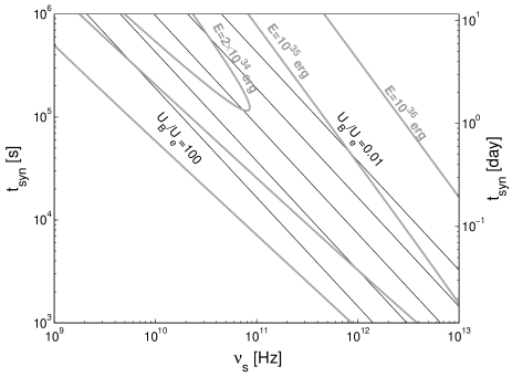
Figure 9.— $U_{{\rm B}}/U_{{\rm e}}$ (black contours) and total energy (gray contours), $E=4/3\pi R^{3}(U_{{\rm e}}+U_{{\rm B}})$, as a function of $\nu_{{\rm s}}$ and $t_{{\rm syn}}$, and assuming $d=1$ kpc, and $S_{\nu}=0.4$ mJy. The equal $U_{{\rm B}}/U_{{\rm e}}$ lines are 100, 10, 1, 0.1, and 0.01 from left to right.

It is interesting to compare the derived radius, $R\approx 6\times 10^{10}$ cm, with some typical radii dominating NS physical processes. The light-cylinder radius is:

$$R_{lc}=\frac{c}{2\pi}P\cong 4.8\times 10^{10}\frac{P}{10\,{\rm s}}\,{\rm cm}.$$ (62)

The co-rotation radius of a NS is:

$$R_{cor} = \Big{(}\frac{GM_{{\rm NS}}}{\omega^{2}}\Big{)}^{1/3}$$ (63)

$$\cong 7.8\times 10^{8}\Big{(}\frac{M_{{\rm NS}}}{1.4\,{\rm M}_{\odot}}\Big{)}^{1/3}\Big{(}\frac{P}{10\,{\rm s}}\Big{)}^{2/3}\,{\rm cm}.$$ (64)

Assuming a Bondi-Hoyle accretion rate:

$$\dot{M}=\frac{4\pi G^{2}M_{{\rm NS}}^{2}m_{p}n_{ISM}}{(V^{2}+c_{{\rm s}}^{2})^{3/2}},$$ (65)

where $m_{p}$ is the proton mass, then the Magnetosphere radius is:

$$R_{m} = \Big{(}\frac{\mu^{2}}{\dot{M}\sqrt{2GM_{{\rm NS}}}}\Big{)}^{2/7}$$ (66)

$$\cong 2.1\times 10^{11}\Big{(}\frac{\mu}{4\times 10^{30}}\Big{)}^{4/7}\Big{(}\frac{\dot{M}}{2\times 10^{8}\,{\rm gr}\,{\rm s}^{-1}}\Big{)}^{-2/7}$$ (68)

$$\times\Big{(}\frac{M_{{\rm NS}}}{1.4\,{\rm M}_{\odot}}\Big{)}^{-1/7}\,{\rm cm},$$

where $\mu$ is the magnetic dipole moment of the NS. Finally, the accretion radius is:

$$R_{{\rm acc}} \approx \frac{2GM_{{\rm NS}}}{V^{2}}$$ (69)

$$\approx 1.7\times 10^{12}\frac{M_{{\rm NS}}}{1.4\,{\rm M}_{\odot}}\Big{(}\frac{V}{150\,{\rm km}\,{\rm s}^{-1}}\Big{)}^{-2}\,{\rm cm}.$$ (70)

As noted at the beginning of the sub-section rapid expansion of the radiating plasma would vastly increase the energy budget. For this reason, an integral requirement of the incoherent model is that the plasma must be confined (in which case the duration of the event is set by the cooling time or by the duration of the injection of energy by the source). We note that the confinement radius should probably be smaller than the light cylinder radius. Otherwise, the energy requirement will be larger due to the inertia of the electrons. The equipartition radius we find (Eq. 49) is a little bit larger than the plausible confinement radius (e.g., Eq. 62). However, our calculation provides only an order of a magnitude estimate to the fireball parameters and the equipartition radius in particular. Therefore, we cannot rule out the incoherent synchrotron model based on the small inconsistency between the equipartition radius and light cylinder radius.

Assuming a dipole magnetic field, decaying as $R^{-3}$ (inside the light cylinder radius; Eq. 62), and $B=17$ G at $R=6\times 10^{10}$ cm, the extrapolated magnetic field strength on the surface of a 10 km radius NS will be about:

$$B(10\,{\rm km}) \approx B\Big{(}\frac{R}{10\,{\rm km}}\Big{)}^{3}$$ (71)

$$\approx 4\times 10^{15}\Big{(}\frac{\nu_{{\rm s}}}{2\times 10^{11}\,{\rm Hz}}\Big{)}^{-4/3}\Big{(}\frac{t_{{\rm syn}}}{0.5\,{\rm day}}\Big{)}^{-7/6}$$ (73)

$$\times\Big{(}\frac{S_{\nu}}{0.4\,{\rm mJy}}\Big{)}^{3/2}\Big{(}\frac{d}{1\,{\rm kpc}}\Big{)}^{3}\,{\rm G}.$$

This is higher than the typical estimated surface magnetic fields of pulsars and Magnetars. However, for somewhat larger $\nu_{{\rm s}}$ or $t_{{\rm syn}}$ the discrepancy is smaller. Moreover, the events may be related to the release of magnetic energy stored in the NS interior. Therefore, we conclude that the incoherent synchrotron model cannot be ruled out.

Finally, we note that the total mass of matter within the emission radius is $4/3\pi n_{{\rm e}}m_{p}R^{3}\sim 4\times 10^{14}$ gr. Interestingly, this mass is similar to the total amount of matter that a NS with a space velocity of 150 km s^-1 will accrete from the ISM (assuming $n=0.1$ cm^-3 and Bondi-Hoyle accretion) within several months, which is the typical time interval between bursts that we found in §6.3. We note that Treves, Colpi & Lipunov (1993) suggested that accreted matter from the ISM is piled up near the Alfvén radius, followed by infall of the piled up matter on the NS. They estimated that these episodic infalls may occur every several months.

6.5. Flares from intermittent pulsars

In recent years, several types of pulsars with small duty cycles have been discovered. This includes the RRATs (McLaughlin et al. 2006), and intermittent pulsars (Kramer et al. 2006). Several models were suggested to explain such episodic pulsars (e.g., Treves et al 1993; Zhang, Gil & Dyks 2006; Cordes & Shannon 2008). However, their evolutionary status is still unclear.

Known intermittent pulsars and RRATs have characteristic ages similar to those of “normal” pulsars (i.e., $\mathrel{\raise 1.29167pt\hbox{$<$}\mkern-14.0mu\lower 2.58334pt\hbox{$\sim$}}10^{7}$ yr). However, as we discussed in §6.2, the long-duration radio transients cannot be associated exclusively with pulsars younger than about 1 Gyr, otherwise their predicted surface density will not be consistent with the observations (§4.2).

As shown in §6.3, in the framework of Galactic NSs, the duty cycle of the long-duration radio transients is $\sim 7\times 10^{-3}$. Such a small duty cycle will make it hard to detect them as repeaters in current pulsars searches. In addition, most pulsar searches are conducted at low frequencies ($\mathrel{\raise 1.29167pt\hbox{$<$}\mkern-14.0mu\lower 2.58334pt\hbox{$\sim$}}1.4$ GHz), in which the rate of the long-duration radio transients seems to be low. Thus, a prediction of this model is that high frequency (say 5 GHz) searches should find a much larger rate of long duration radio transients.

The flat spectrum ($\alpha\mathrel{\raise 1.29167pt\hbox{$>$}\mkern-14.0mu\lower 2.58334pt\hbox{$\sim$}}0$) of the long duration transients is reminiscent of the radio spectrum of magnetars in their “active state” (cf. Camilo et al. 2006). Thus, a plausible model is that the long duration transients are ancient magnetars in short lived high states.

6.6. The distance scale to the Kida et al. transients

Next we derive a physical distance to the bright events discussed by Kida et al. (2008). We remind the reader that these events are about a thousand times brighter than the VLA events. We use a modified Rayleigh test (see Fisher et al. 1987) to compare the sky distribution of the Kida et al. (2008) transients with that of the celestial positions of simulated NSs:

$$(\sum_{i=1}^{6}{\sin[b_{i}]})^{2}\equiv\Sigma^{2}b,$$ (74)

for the sample of six radio transients found by Kida et al. (2008); here $b$ is the Galactic latitude.

Next, we selected from the Heliocentric catalog of simulated isolated-old NSs of Ofek (2009), six random NSs within the footprints of the Kida et al. search zone, found up to a distance $d$ from the Sun and calculated their $\Sigma^{2}b$. We assume that the survey described in Kida et al. (2008) covers the entire declination zone $\delta=32^{\circ}-42^{\circ}$ equally. For each distance $d$, in the range of 100 pc to 10 kpc, we repeated this process 10,000 times. In Figure 10, we show the mean expected value, and the $68$, $95$ and $99.73$ percentiles, for the distribution of $\Sigma^{2}b$ of simulated NSs as a function of distance. As can be gathered from Figure 10 the typical distance to these events is below 150 pc (900 pc), at the $68\%$ ($95\%$) CL.

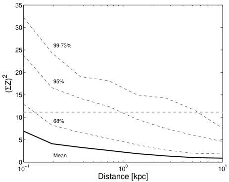
Figure 10.— The sky uniformity of the Kida et al. transients (described by $\Sigma^{2}b$; Eq. 74) as a function of the distance to the transients. The gray-thick dashed line shows the value calculated for the observed sample. The black line shows the mean value calculated for the simulated NSs, while the gray-thin dashed lines show the upper $68$, $95$ and $99.73$ percentiles (from bottom up) of the distribution of the uniformity criterion $\Sigma^{2}{b}$ of the simulated NSs. The lines fluctuates due to the limited statistics.

Kida et al. reported six events in their survey which covers about $7\%$ of the celestial sphere. Therefore, the all-sky surface density of the Kida et al. transients is $\mathrel{\raise 1.29167pt\hbox{$>$}\mkern-14.0mu\lower 2.58334pt\hbox{$\sim$}}30$ sources at the $95\%$ confidence. Ofek (2009) found that the density of NSs in the solar neighborhood is $2\times 10^{-4}$ pc^-3 assuming $10^{9}$ NS in the Galaxy and the Arzoumanian et al. (2002) initial velocity distribution. At small distances ($\mathrel{\raise 1.29167pt\hbox{$<$}\mkern-14.0mu\lower 2.58334pt\hbox{$\sim$}}100$ pc) the distribution of NSs around the Sun is near isotropic. Therefore, by comparing the density from the simulations with the observed surface density of the Kida et al. (2008) events, we put a lower limit on the distance to the Kida et al. (2008) event, assuming they originate from Galactic NSs, of $\mathrel{\raise 1.29167pt\hbox{$>$}\mkern-14.0mu\lower 2.58334pt\hbox{$\sim$}}30$ pc at the 95$\%$ CL.

7. Summary

We review several recent discoveries of radio transients with durations between minutes to days (Kuniyoshi et al. 2006; Bower et al. 2007; Niinuma et al. 2007; Kida et al. 2008). We suggest that these radio transients may be generated by a single class of progenitors. The main characteristics of these “long duration radio transients” are: (i) a very high occurrence rate of about $\sim 10^{3}$ deg^-2 yr^-1 in the 5-GHz band; (ii) common at intermediate Galactic latitude, with progenitors sky surface density of $\mathrel{\raise 1.29167pt\hbox{$>$}\mkern-14.0mu\lower 2.58334pt\hbox{$\sim$}}60$ deg^-2 at Galactic latitude, $b\sim 40^{\circ}$; (iii) lacking any X-ray ($\mathrel{\raise 1.29167pt\hbox{$>$}\mkern-14.0mu\lower 2.58334pt\hbox{$\sim$}}10^{-13}$ erg cm^-2 s^-1), visible light ($g<27.6$, $R<26.5$ mag), near-IR ($K<20.4$ mag) and radio ($S_{5\,{\rm GHz}}\mathrel{\raise 1.29167pt\hbox{$>$}\mkern-14.0mu\lower 2.58334pt\hbox{$\sim$}}10\,\mu$Jy) counterparts; and (iv) more abundant in the 5-GHz band as compared to that in the 1.4-GHz band; From the rates in the two bands we infer the spectral index between the two bands is $\alpha\mathrel{\raise 1.29167pt\hbox{$>$}\mkern-14.0mu\lower 2.58334pt\hbox{$\sim$}}0$ where the flux density, $f_{\nu}\propto\nu^{\alpha}$.

These events are most probably not associated with the usual culprits like GRBs, SGRs, AGNs, SNe, flare stars, pulsars and interacting binaries (§5). We find that several other hypothesis including Galactic isolated old NS; brown dwarfs and some sort of a new kind of explosions cannot be ruled out. Among these, we find that the association with isolated old NSs is especially attractive. We explore this hypothesis in details and show that it is consistent with the current observations. In the framework of Galactic isolated old NSs we show that: (i) the typical distance to the Bower et al. sample (mJy events) is between 1 kpc and $\sim 5$ kpc; (ii) the typical distance to the Kida et al. Jy-level events is less than about 0.9 kpc and more than 30 pc at the $95\%$ CL; and (iii) they will have a burst repetition time scale of about several months and duty cycle of $\sim 7\times 10^{-3}$.

A possible association with isolated old NS is exciting. If correct, this may prove to be the most practical way, so far, to find old NSs in our Galaxy and explore their demographics. Specifically, the demography of old NSs constitute an excellent probe of the star formation history and metal enrichment of the Galaxy, and the gravitational potential of the Galaxy.

Our analysis naturally suggests several tests that can be used to rule out this hypothesis. First, if indeed long-duration radio transients are associated with isolated old NSs, then we expect them to be distributed inhomogeneously on the celestial sphere. Specifically, this hypothesis predicts that faint sub-mJy long-duration radio transients will be at least a few times more common in the Galactic center than in high Galactic latitude. The exact ratio, however, depends on the distance scale to these events. This is illustrated in Figure 6 which shows the expected approximate distribution of isolated old NSs on the celestial sphere, for the entire NS population and NS which are at distance smaller than 1 kpc from the Sun. Finally, we note that if the radio emission from such sources is pulsating, then pulsars searches conducted at 5 GHz will find these objects. The fact that such “pulsars” were not found in existing surveys may be due to the fact that the majority of pulsars searches are carried on in low frequencies in which the rate of these transients is low.

References

- Agüeros et al. (2006) Agüeros, M. A., et al. 2006, AJ, 131, 1740
- Arnett et al. (1989) Arnett, W. D., Schramm, D. N., & Truran, J. W. 1989, ApJL, 339, L25
- Arons & Lea (1976) Arons, J., & Lea, S. M. 1976, ApJ, 207, 914
- Arons & Lea (1980) Arons, J., & Lea, S. M. 1980, ApJ, 235, 1016
- Arzoumanian et al. (2002) Arzoumanian, Z., Chernoff, D. F., & Cordes, J. M. 2002, ApJ, 568, 289
- Baraffe et al. (2003) Baraffe, I., Chabrier, G., Barman, T. S., Allard, F., & Hauschildt, P. H. 2003, A&A, 402, 701
- Barbary et al. (2009) Barbary, K., et al. 2009, ApJ, 690, 1358
- Bastian et al. (1998) Bastian, T. S., Benz, A. O., & Gary, D. E. 1998, ARA&A, 36, 131
- Becker et al. (1995) Becker, R. H., White, R. L., & Helfand, D. J. 1995, ApJ, 450, 559
- Berger et al. (2001) Berger, E., et al. 2001, Nature, 410, 338
- Berger (2002) Berger, E. 2002, ApJ, 572, 503
- Berger et al. (2005) Berger, E., et al. 2005, ApJ, 627, 960
- Berger (2006) Berger, E. 2006, ApJ, 648, 629
- Berger et al. (2008a) Berger, E., et al. 2008a, ApJ, 673, 1080
- Berger et al. (2008b) Berger, E., et al. 2008b, ApJ, 676, 1307
- Blaes & Madau (1993) Blaes, O., & Madau, P. 1993, ApJ, 403, 690
- Bondi & Hoyle (1944) Bondi, H., & Hoyle, F. 1944, MNRAS, 104, 273
- Bower et al. (2007) Bower, G. C., Saul, D., Bloom, J. S., Bolatto, A., Filippenko, A. V., Foley, R. J., & Perley, D. 2007, ApJ, 666, 346
- Burgasser et al. (2000) Burgasser, A. J., Kirkpatrick, J. D., Reid, I. N., Liebert, J., Gizis, J. E., & Brown, M. E. 2000, AJ, 120, 473
- Burgasser (2004) Burgasser, A. J. 2004, ApJS, 155, 191
- Burgasser & Putman (2005) Burgasser, A. J., & Putman, M. E. 2005, ApJ, 626, 486
- Burrows et al. (1997) Burrows, A., et al. 1997, ApJ, 491, 856
- Cameron et al. (2005) Cameron, P. B., et al. 2005, Nature, 434, 1112
- Camilo et al. (2006) Camilo, F., Ransom, S. M., Halpern, J. P., Reynolds, J., Helfand, D. J., Zimmerman, N., & Sarkissian, J. 2006, Nature, 442, 892
- Carilli et al. (2003) Carilli, C. L., Ivison, R. J., & Frail, D. A. 2003, ApJ, 590, 192
- Cenko et al. (2008) Cenko, S. B., et al. 2008, ApJ, 677, 441
- Chandra et al. (2008) Chandra, P., et al. 2008, ApJ, 683, 924
- Chanmugam (1992) Chanmugam, G. 1992, ARA&A, 30, 143
- Cole et al. (2001) Cole, S., et al. 2001, MNRAS, 326, 255
- Colgate (1975) Colgate, S. A. 1975, ApJ, 198, 439
- Colgate & Noerdlinger (1971) Colgate, S. A., & Noerdlinger, P. D. 1971, ApJ, 165, 509
- Colpi et al. (1998) Colpi, M., Turolla, R., Zane, S., & Treves, A. 1998, ApJ, 501, 252
- Condon et al. (1998) Condon, J. J., Cotton, W. D., Greisen, E. W., Yin, Q. F., Perley, R. A., Taylor, G. B., & Broderick, J. J. 1998, AJ, 115, 1693
- Cordes & Chernoff (1998) Cordes, J. M., & Chernoff, D. F. 1998, ApJ, 505, 315
- Cordes & Shannon (2008) Cordes, J. M., & Shannon, R. M. 2008, ApJ, 682, 1152
- Deneva et al. (2008) Deneva, J. S., et al. 2008, arXiv:0811.2532
- DeBoer et al. (2004) DeBoer, D. R., et al. 2004, Proc. SPIE, 5489, 1021
- Eichler (2002) Eichler, D. 2002, MNRAS, 335, 883
- Falcke et al. (2007) Falcke, H. D., et al. 2007, Highlights of Astronomy, 14, 386
- Faucher-Giguère & Kaspi (2006) Faucher-Giguère, C.-A., & Kaspi, V. M. 2006, ApJ, 643, 332
- Fisher et al. (1987) Fisher, N. I., Lewis, T., & Embleton, B. J. J. 1987, Cambridge: University Press, 1987,
- Frail et al. (1997) Frail, D. A., et al. 1997, ApJL, 483, L91
- Fruchter et al. (2006) Fruchter, A. S., et al. 2006, Nature, 441, 463
- Galama et al. (1997) Galama, T. J., de Bruyn, A. G., van Paradijs, J., Hanlon, L., & Bennett, K. 1997, A&A, 325, 631
- Gal-Yam et al. (2006) Gal-Yam, A., et al. 2006, ApJ, 639, 331
- Gehrels (1986) Gehrels, N. 1986, ApJ, 303, 336
- Gehrels et al. (2004) Gehrels, N., et al. 2004, ApJ, 611, 1005
- Ghez et al. (2008) Ghez, A. M., et al. 2008, ApJ, 689, 1044
- Goldreich & Julian (1969) Goldreich, P., & Julian, W. H. 1969, ApJ, 157, 869
- Gould et al. (1996) Gould, A., Bahcall, J. N., & Flynn, C. 1996, ApJ, 465, 759
- Gregg et al. (2002) Gregg, M. D., Lacy, M., White, R. L., Glikman, E., Helfand, D., Becker, R. H., & Brotherton, M. S. 2002, ApJ, 564, 133
- Güdel (2002) Güdel, M. 2002, ARA&A, 40, 217
- Guetta et al. (2005) Guetta, D., Piran, T., & Waxman, E. 2005, ApJ, 619, 412
- Haberl et al. (1998) Haberl, F., Motch, C., & Pietsch, W. 1998, Astronomische Nachrichten, 319, 97
- Hallinan et al. (2007) Hallinan, G., et al. 2007, ApJL, 663, L25
- Harrison et al. (1999) Harrison, F. A., et al. 1999, ApJL, 523, L121
- Hawking (1974) Hawking, S. W. 1974, Nature, 248, 30
- Helfand et al. (1980) Helfand, D. J., Chanan, G. A., & Novick, R. 1980, Nature, 283, 337
- Hopkins & Beacom (2006) Hopkins, A. M., & Beacom, J. F. 2006, ApJ, 651, 142
- Hyman et al. (2005) Hyman, S. D., Lazio, T. J. W., Kassim, N. E., Ray, P. S., Markwardt, C. B., & Yusef-Zadeh, F. 2005, Nature, 434, 50
- Hyman et al. (2009) Hyman, S. D., Wijnands, R., Lazio, T. J. W., Pal, S., Starling, R., Kassim, N. E., & Ray, P. S. 2009, ApJ, 696, 280
- Ikhsanov (2007) Ikhsanov, N. R. 2007, Ap&SS, 308, 137
- Johns-Krull & Valenti (1996) Johns-Krull, C. M., & Valenti, J. A. 1996, ApJL, 459, L95
- Jørgensen et al. (2002) Jørgensen, P. S., Riis, T., Betto, M., & Pickles, A. 2002, Astronomical Data Analysis Software and Systems XI, 281, 207
- Kellermann & Pauliny-Toth (1969) Kellermann, K. I., & Pauliny-Toth, I. I. K. 1969, ApJL, 155, L71
- Kida et al. (2008) Kida, S., et al. 2008, New Astronomy, 13, 519
- Kinney et al. (1996) Kinney, A. L., Calzetti, D., Bohlin, R. C., McQuade, K., Storchi-Bergmann, T., & Schmitt, H. R. 1996, ApJ, 467, 38
- Kramer et al. (2006) Kramer, M., Lyne, A. G., O’Brien, J. T., Jordan, C. A., & Lorimer, D. R. 2006, Science, 312, 549
- Kulkarni et al. (1998) Kulkarni, S. R., et al. 1998, Nature, 395, 663
- Kulkarni et al. (2009) Kulkarni, S. R., Ofek, E. O., Neill, D., Juric, M., Zheng, Z., in prep.
- Kuniyoshi et al. (2006) Kuniyoshi, M., et al. 2006, PASP, 118, 901
- Levinson et al. (2002) Levinson, A., Ofek, E. O., Waxman, E., & Gal-Yam, A. 2002, ApJ, 576, 923
- Lorimer et al. (2007) Lorimer, D. R., Bailes, M., McLaughlin, M. A., Narkevic, D. J., & Crawford, F. 2007, Science, 318, 777
- Maoz et al. (1997) Maoz, D., Ofek, E. O., & Shemi, A. 1997, MNRAS, 287, 293
- McLaughlin et al. (2006) McLaughlin, M. A., et al. 2006, Nature, 439, 817
- Motch et al. (1997) Motch, C., Guillout, P., Haberl, F., Pakull, M., Pietsch, W., & Reinsch, K. 1997, A&A, 318, 111
- Nakar et al. (2006) Nakar, E., Gal-Yam, A., Piran, T., & Fox, D. B. 2006, ApJ, 640, 849
- Narayan & Ostriker (1990) Narayan, R., & Ostriker, J. P. 1990, ApJ, 352, 222
- Niinuma et al. (2007) Niinuma, K., et al. 2007, ApJL, 657, L37
- Ofek (2007) Ofek, E. O. 2007, ApJ, 659, 339
- Ofek et al. (2006) Ofek, E. O., et al. 2006, ApJ, 652, 507
- Ofek et al. (2008) Ofek, E. O., et al. 2008, ApJ, 681, 1464
- Ofek (2009) Ofek, E. O. 2009, PASP, 121, 814
- Ostriker et al. (1970) Ostriker, J. P., Rees, M. J., & Silk, J. 1970, ApL, 6, 179
- Ovaldsen et al. (2007) Ovaldsen, J.-E., et al. 2007, ApJ, 662, 294
- Perley et al. (2009) Perley, D. A., et al. 2009, arXiv:0905.0001
- Perna et al. (2003) Perna, R., Narayan, R., Rybicki, G., Stella, L., & Treves, A. 2003, ApJ, 594, 936
- Peterson (1997) Peterson, B. M. 1997, An introduction to active galactic nuclei, Publisher: Cambridge, New York Cambridge University Press, 1997 Physical description xvi, 238 p. ISBN 0521473489
- Phinney & Kulkarni (1994) Phinney, E. S., & Kulkarni, S. R. 1994, ARA&A, 32, 591
- Phinney & Taylor (1979) Phinney, S., & Taylor, J. H. 1979, Nature, 277, 117
- Popov & Stern (2006) Popov, S. B., & Stern, B. E. 2006, MNRAS, 365, 885
- Press et al. (1992) Press, W. H., Teukolsky, S. A., Vetterling, W. T., & Flannery, B. P. 1992, Cambridge: University Press, —c1992, 2nd ed.
- Quimby et al. (2009) Quimby, R. M., et al. 2009, submitted to Nature, arXiv:0910.0059
- Rees (1977) Rees, M. J. 1977, Nature, 266, 333
- Readhead (1994) Readhead, A. C. S. 1994, ApJ, 426, 51
- Reid et al. (1999) Reid, I. N., et al. 1999, ApJ, 521, 613
- Reyes et al. (2008) Reyes, R., et al. 2008, AJ, 136, 2373
- Rutledge et al. (2003) Rutledge, R. E., Fox, D. W., Bogosavljevic, M., & Mahabal, A. 2003, ApJ, 598, 458
- Rybicki & Lightman (1979) Rybicki, G. B., & Lightman, A. P. 1979, New York, Wiley-Interscience, 1979. 393 p.
- Sagiv & Waxman (2002) Sagiv, A., & Waxman, E. 2002, ApJ, 574, 861
- Sengupta (1997) Sengupta, S. 1997, ApJL, 479, L133
- Soderberg et al. (2006) Soderberg, A. M., et al. 2006, Nature, 442, 1014
- Srinivasan (1989) Srinivasan, G. 1989, A&ARv, 1, 209
- Sun & Han (2002) Sun, X., & Han, J. 2002, Progress in Astronomy, 20, 130
- Toropina et al. (2001) Toropina, O. D., Romanova, M. M., Toropin, Y. M., & Lovelace, R. V. E. 2001, ApJ, 561, 964
- Toropina et al. (2003) Toropina, O. D., Romanova, M. M., Toropin, Y. M., & Lovelace, R. V. E. 2003, ApJ, 593, 472
- Toropina et al. (2005) Toropina, O. D., Romanova, M. M., Toropin, Y. M., & Lovelace, R. V. E. 2005, Memorie della Societa Astronomica Italiana, 76, 508
- Treves & Colpi (1991) Treves, A., & Colpi, M. 1991, A&A, 241, 107
- Treves et al. (1993) Treves, A., Colpi, M., & Lipunov, V. M. 1993, A&A, 269, 319
- Treves et al. (2001) Treves, A., Popov, S. B., Colpi, M., Prokhorov, M. E., & Turolla, R. 2001, X-ray Astronomy 2000, 234, 225
- Urpin & Muslimov (1992) Urpin, V. A., & Muslimov, A. G. 1992, MNRAS, 256, 261
- Vachaspati (2008) Vachaspati, T. 2008, Physical Review Letters, 101, 141301
- Valenti et al. (1995) Valenti, J. A., Marcy, G. W., & Basri, G. 1995, ApJ, 439, 939
- Voges et al. (1999) Voges, W., et al. 1999, A&A, 349, 389
- Voges et al. (2000) Voges, W., et al. 2000, IAUC, 7432, 3
- Weiler et al. (1991) Weiler, K. W., van Dyk, S. D., Discenna, J. L., Panagia, N., & Sramek, R. A. 1991, ApJ, 380, 161
- White et al. (1997) White, R. L., Becker, R. H., Helfand, D. J., & Gregg, M. D. 1997, ApJ, 475, 479
- Yakovlev & Pethick (2004) Yakovlev, D. G., & Pethick, C. J. 2004, ARA&A, 42, 169
- Zhang et al. (2007) Zhang, B., Gil, J., & Dyks, J. 2007, MNRAS, 374, 1103