Chiral EFT with a resonance and heavy fields

Abstract:

Several conceptual points concerning the inclusion of the $\Delta$(1232) resonance in the framework of chiral effective-field theory are discussed, with an emphasis on the problem of power counting in the baryon sector in general. I also formulate a new dispersion relation in the pion-mass squared (or, the quark mass) and make a link between the power counting and the analytic properties of chiral expansion. A controversy regarding the determination of the proton’s magnetic polarizability from Compton-scattering data is stressed here as well.

1 Introduction

The limit of applicability of chiral perturbation theory ($\chi$PT) [1, 2, 3] is ultimately set by the scale of spontaneous chiral symmetry breaking: $\Lambda_{\chi SB}\simeq 4\pi f_{\pi}\sim 1$ GeV, but not only. Resonances with excitation energy lower than 1 GeV, e.g. $\rho$(770) or $\Delta$(1232), set a lower limit, if not included explicitly. The $\Delta$(1232) is especially important because of its very low excitation energy, as defined by the $\Delta$-nucleon mass splitting:

$$\varDelta\equiv M_{\Delta}-M_{N}\approx(1232-939)\,\mbox{MeV}=293\,\mbox{MeV.}$$ (1)

This means we can expect an early breakdown of $\chi$PT in the baryon sector, on one hand, but an easy fit of the $\Delta$ into the $\chi$PT power-counting scheme ($\varDelta\ll\Lambda_{\chi SB}$), on the other.

A first work on the inclusion of $\Delta$-resonance and, more generally, the decuplet fields in $\chi$PT was done by Jenkins and Manohar [4], who at the same time developed the “heavy-baryon” (HB) expansion [5]. They counted the $\Delta$-excitation scale to be of the same order as other light scales in the theory, i.e., Goldstone-boson momenta and masses. For the two-flavor QCD, this hierarchy of scales,

$$\varDelta\sim p\sim m_{\pi}\ll\Lambda_{\chi SB}\,,$$ (2)

results in the “small scale expansion” (SSE) [6].

Alternatively, one can count the resonance excitation scale to be different from the pion mass, i.e.,

$$m_{\pi}<\varDelta\ll\Lambda_{\chi SB}\,.$$ (3)

This is an example of effective-field theory (EFT) with two distinct light scales. The power counting of graphs will then depend on whether the typical momenta are comparable to $m_{\pi}$ or to $\varDelta$. The expansion can be carried out in terms of one small parameter, e.g.,

$$\delta=\frac{\varDelta}{\Lambda_{\chi SB}}\ll 1\,.$$ (4)

Then, $m_{\pi}/\Lambda_{\chi SB}$ should count as $\delta$ to some power greater than one. The simplest is to take an integer power:

$$\frac{m_{\pi}}{\Lambda_{\chi SB}}\sim\delta^{2}.$$ (5)

This counting scheme goes under the name of “$\delta$-expansion” [7].

The main advantage of the $\delta$-expansion over the SSE is that it provides a more adequate counting of the resonant contributions and a power-counting argument to sum a subset of graphs generating the resonance width.

In Sect. 4 we shall see a brief account of one recent applications of the $\delta$-expansion, a new calculation of the $\Delta$-resonance effect on the nucleon polarizabilities and Compton scattering off protons [8]. More applications can be found elsewhere [9, 10, 11, 12], including these proceedings [13]. The other purpose of this paper is to remark on two, quite unrelated, consistency problems of $\chi$PT in the baryon sector (B$\chi$PT). One concerns the treatment of higher-spin fields (Sect. 2), and the other is about the power counting (Sect. 3 and 4).

2 Higher-spin fields

Including the baryon field in the chiral Lagrangian, one sooner or later faces the consistency problems of higher-spin field theory. The $\Delta$(1232), being a spin-3/2 state, can be represented by a Rarita-Schwinger (RS) vector-spinor, $\psi_{\alpha}(x)$, with the following free Lagrangian:

$$\mathcal{L}_{RS}=\bar{\psi}_{\alpha}\,(i\,\gamma^{\alpha\beta\varrho}\partial_{\varrho}-M_{\Delta}\,\gamma^{\alpha\beta})\,\psi_{\beta},$$ (6)

where $\gamma^{\alpha\beta\rho}$ and $\gamma^{\alpha\beta}$ are totally antisymmetrized products of three and two Dirac matrices. The Lagrangian consists of a kinetic term, which is invariant under a gauge symmetry:

$$\psi_{\alpha}\to\psi_{\alpha}+\partial_{\alpha}\epsilon$$ (7)

(with a spinor $\epsilon$), and a mass term, which breaks the gauge symmetry. This formalism provides a proper field-theoretic description of a spin-3/2 particle. The symmetry ensures that the massless particle has 2 spin degrees of freedom, while the mass term breaks it such as to raise the number of spin degrees of freedom to 4. This pattern has to be preserved by interactions of this field, but such a consistency criterion proved to be tough to fulfill.

For instance, the usual minimal substitution of the electromagnetic field, $\partial_{\rho}\to\partial_{\rho}+ieA_{\rho}$, leads to U(1)-invariant theory, but at expense of loss of the spin-3/2 gauge symmetry of massless theory. As the result, all hell, with its negative-norm states [14], superluminal modes [15], etc. [16], breaks loose. Naive attempts to restore the spin-3/2 gauge symmetry break the U(1) gauge symmetry, and so on. In fact, there are ‘no-go theorems’ forbidding a consistent coupling of a spin-3/2 field to electromagnetism without gravity, see e.g., [17].

This situation is frustrating, especially since we would like to couple the $\Delta$’s to pions too, and so, chiral symmetry is one more symmetry to worry about. Fortunately, ‘locality’ is one of the principles that underlines the ‘no-go theorem’, and, given that the EFT framework is essentially non-local, we have a way to work around it. One method has been outlined in Ref. [18] (Sect. 4.2 therein), and a similar method has been developed in parallel [19]. However, a complete closed-form solution to this problem is still lacking.

3 Heavy fields and dispersion in the pion mass

Another important issue of concern is the treatment of heavy fields in $\chi$PT. This problem comes already with the inclusion of the nucleon field. A key question is: ”how to count derivatives of the nucleon field?” The nucleon is heavy ($M_{\,N}\sim{\Lambda}_{\chi SB}$), and hence the time (0th) component of the nucleon derivative, or momentum, is much greater than the spatial components:

$$\partial_{i}N(x)\ll\partial_{0}N(x),$$ (8)

or, in the momentum space, $p\ll\sqrt{M_{N}^{2}+p^{2}}$, for an on-shell nucleon. It would be correct to count the 0th component as $\mathcal{O}(1)$, while the spatial components as $\mathcal{O}(p)$, but this counting obviously does not respect the Lorentz invariance.

In a Lorentz-invariant formulation, $\partial_{\mu}N$ counts as $\mathcal{O}(1)$, except when in a particular combination, $(i\partial\!\!\!\!\!/-M_{N})N$, which counts as $\mathcal{O}(p)$. This counting has a consistency problem, as can be seen from the following example. Consider an expression, $P_{\mu}-M_{N}\gamma_{\mu}$, where $P_{\mu}$ here is the nucleon four-momentum which, as $\gamma_{\mu}$ and $M_{N}$, counts as 1. The counting of this expression, as a whole, will unfortunately depend on how it is contracted. E.g., whether contracted with $p$ or $\gamma$ we have:

$$P^{\mu}(P_{\mu}-M_{N}\gamma_{\mu})=P\!\!\!\!\!/\,(P\!\!\!\!\!/\,-M_{N}) \sim \mathcal{O}(p),$$

$$\gamma^{\mu}(P_{\mu}-M_{N}\gamma_{\mu})=-3M_{N}+(P\!\!\!\!\!/\,-M_{N}) \sim \mathcal{O}(1).$$

This inconsistency leads eventually to the appearance of nominally lower-order or higher-order contributions than ones expected from power-counting [3].

The heavy-baryon (HB) expansion of Jenkins and Manohar [5] overcomes this problem, but again, at the expense of manifest Lorentz-invariance. In HB$\chi$PT one writes

$$P_{\mu}=M_{N}v_{\mu}+\ell_{\mu}$$ (9)

with $v=(1,0,0,0)$, which allows to assign a consistent power to $\ell$.

More recently it is becoming increasingly clear that the power-counting problem of Lorentz-invariant formulation is not very severe [20], or perhaps not a problem at all [21]. The lower-order ‘power-counting violating’ contributions come out to be analytic in quark masses, and therefore match the contributions that come multiplying the low-energy constants (LECs), and as result, do not play any role other than renormalizing the LECs. The higher-order contributions, on the other hand, can be both analytic and non-analytic in quark masses. Their analytic parts may contain ultra-violet divergencies, so one needs to define the renormalization scheme for the higher-order LECs, before they actually appear in the calculation. The non-analytic parts are most interesting, as they may come with unnaturally large coefficients, and therefore cannot be dismissed as ‘higher order’ at all.

Figure 1: The nucleon self-energy contribution at order $p^{3}$.

This discussion is nicely illustrated by the classic example of chiral corrections to the nucleon mass. Up to $\mathcal{O}(p^{3})$ this expansion is given by

$$M_{N}={M}_{N0}-4c_{1}m_{\pi}^{2}+\Sigma^{(3)}_{N},$$ (10)

where ${M}_{N0}$ and $c_{1}$ are LECs which, supposedly, represent the values of nucleon mass and $\pi N$ $\sigma$-term in the chiral limit. The last term is the (leading) 3rd-order self-energy correction, Fig. 1:

$$\Sigma^{(3)}_{N} = \left.i\,\frac{3g_{A}^{2}}{4f_{\pi}^{2}}\int\!\frac{d^{4}k}{(2\pi)^{4}}\frac{k\!\!\!\!/\gamma_{5}(p\!\!\!\!/-k\!\!\!\!/+M_{N})k\!\!\!\!/\gamma_{5}}{(k^{2}-m_{\pi}^{2})[(p-k)^{2}-M_{N}^{2}]}\right|_{p\!\!\!\!/=M_{N}}$$ (11b)

$$\stackrel{{\scriptstyle\mathrm{dimreg}}}{{=}} \frac{3g_{A}^{2}}{4f_{\pi}^{2}}\frac{M_{N}^{3}}{(4\pi)^{2}}\int\nolimits_{0}^{1}\!dx\,\Big{\{}[x^{2}+\mu^{2}(1-x)]\left(L_{\epsilon}+\ln[x^{2}+\mu^{2}(1-x)]\right)$$

$$\hskip 71.13188pt+\,[2x^{2}-\mu^{2}(2+x)]\left(L_{\epsilon}+1+\ln[x^{2}+\mu^{2}(1-x)]\right)-3L_{\epsilon}\Big{\}},$$

where $\mu=m_{\pi}/M_{N}$, while $L_{\epsilon}=-1/\epsilon-1+\gamma_{E}-\ln(4\pi{\Lambda}/M_{N})$ exhibits the ultraviolet divergence as $\epsilon=(4-d)/2\to 0$, with $d$ being the number of dimensions, ${\Lambda}$ the scale of dimensional regularization, and $\gamma_{E}$ the Euler’s constant. Note that we took the physical nucleon mass for the on-mass-shell condition, as well as for the propagator pole, and not the chiral-limit mass $M_{N0}$, which comes from the Lagrangian. There are several reasons for that (for one, $M_{N}$ is the “known known” here), but in any case the difference between doing it one way or the other is of higher order.

After the integration over $x$ we obtain:

$$\Sigma^{(3)}_{N}=\frac{3g_{A}^{2}M_{N}^{3}}{2(4\pi f_{\pi})^{2}}\left\{-L_{\epsilon}+\left(1-L_{\epsilon}\right)\mu^{2}\right\}\,+\,\overline{\Sigma}^{(3)}_{N},$$ (12a)

with $$\overline{\Sigma}^{(3)}_{N}=-\frac{3g_{A}^{2}M_{N}^{3}}{(4\pi f_{\pi})^{2}}\Big{(}\mu^{3}\sqrt{1-\mbox{\small{$\frac{1}{4}$}}\mu^{2}}\,\,\arccos\mbox{\small{$\frac{1}{2}$}}\mu+\mbox{\small{$\frac{1}{4}$}}\mu^{4}\,\ln\mu^{2}\Big{)}$$ (12b)

$$\,\,\,\,=\,-\frac{3g_{A}^{2}}{(4\pi f_{\pi})^{2}}\frac{1}{2}\Big{[}\pi\,m_{\pi}^{3}-(m_{\pi}^{4}/M_{N})(1-\ln m_{\pi}/M_{N})+\mathcal{O}(m_{\pi}^{5})\Big{]}.$$

Now we can see the problem explicitly. While the power-counting of the graph (Fig. 1) gives order 3, the result contains both lower and higher powers of the light scale, $m_{\,\pi}$.

The higher-order terms should not be a problem. Formally we can either keep them or not without an effect to the accuracy with which we work. There are cases where it is not as simple as that. One such case is considered in the next section.

The lower-order terms, written out in Eq. (12a), have been of a bigger concern [3]. Fortunately, they are of the same form as the first two terms in the expansion of nucleon mass, Eq. (13). Chiral symmetry ensures this “miracle” happens every time. The troublesome lower-order terms can thus be absorbed into a renormalization of the available LECs — a view introduced by Gegelia and Japaridze [21]. In fact, these terms must be absorbed, if $M_{N0}$ and $c_{1}$ are really to represent the values of nucleon mass and $\sigma$-term in the chiral limit. As a result,

$$M_{N}={M}_{N0}-4c_{1}m_{\pi}^{2}+\overline{\Sigma}^{(3)}_{N},$$ (13)

and all is well, from the power-counting point of view. The only question left (in some expert’s minds) is whether these LECs will be renormalized in exact same amounts in calculations of other quantities at this order. In my view, again, the symmetries ensure this is so. I am not aware of an example to the contrary.

Alternatively, the HB formalism [5] yields right away the following expression for the graph of Fig. 1:

$$\Sigma^{(3)HB}_{N}=-\frac{3g_{A}^{2}}{(4\pi f_{\pi})^{2}}\frac{1}{2}\pi\,m_{\pi}^{3},$$ (14)

i.e., only the first term in the expansion of the renormalized self-energy, Eq. (12b). So, no lower-order terms are present (in dimensional regularization!), no higher-order terms either: a perfect consistency with power counting. However, as practice shows, in too many cases the thus neglected higher-order (in $p/M_{N}$) terms are not that small. Unlike in the above-considered example of nucleon mass, the higher powers of $m_{\pi}/M_{N}$ can come with ‘unnaturally large’ coefficients. In these cases, the HB expansion demonstrates poor convergence. One such case — the nucleon polarizabilities — will be considered below, but first, I would like to introduce a principle of analyticity of the chiral expansion.

For this purpose I would like to have a dispersion relation in the variable $t=m_{\,\,\,\pi}^{\,\,\,2}$. It is clear that for negative $t$, the chiral-loop graphs of the type in Fig. 1 will have an imaginary part, reflecting the possibility of decay of the nucleon into itself and a tachionic pion, and hence there is a cut extending from $t=0$ to $t=-\infty$. In the rest of the complex $t$ plane, we can expect an analytic dependence. A dispersion-relation for a quantity such as nucleon self-energy must then read:

$$\mathrm{Re}\,\Sigma_{N}(t)=-\frac{1}{\pi}\int\limits_{-\infty}^{0}dt^{\prime}\,\frac{\mathrm{Im}\,\Sigma_{N}(t^{\prime})}{t^{\prime}-t}$$ (15)

In the above example of 3rd order self-energy, we can easily find the imaginary part from Eq. (11b), if we restore the $i\epsilon$ prescription and use $\ln(-1+i\epsilon)=i\pi$,

$$\mathrm{Im}\,\Sigma_{N}^{(3)}(t)=\frac{3g_{A}^{2}}{(4\pi f_{\pi})^{2}}\frac{\pi}{2}\left[-(-t)^{3/2}\left(1-\frac{t}{4M_{N}^{2}}\right)^{1/2}\!+\,\frac{t^{2}}{2M_{N}}\right]\,\theta(-t)\,.$$ (16)

According to the expansion Eq. (13), we should be making at least two subtractions at $t=0$, and hence

$$\mathrm{Re}\,\overline{\Sigma}_{N}(t)=\mathrm{Re}\,\Sigma_{N}(t)-\mathrm{Re}\,\Sigma_{N}(0)-\mathrm{Re}\,\Sigma_{N}^{\prime}(0)\,\,t\,=\,-\frac{1}{\pi}\int\limits_{-\infty}^{0}dt^{\prime}\,\frac{\mathrm{Im}\,\Sigma_{N}(t^{\prime})}{t^{\prime}-t}\left(\frac{t}{t^{\prime}}\right)^{2}.$$ (17)

Substituting the expression for the imaginary part, and taking $t=m_{\,\,\,\pi}^{\,\,\,2}$, we indeed recover the result of Eq. (12b), therefore validating the analyticity assumptions on one hand, and revealing the intricate nature of the ‘higher-order terms’ on the other.

4 Compton scattering and proton polarizabilities

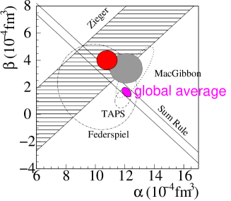
Figure 2: The scalar polarizabilities of the proton. The results of HB$\chi$PT [30] and B$\chi$PT [8] are shown respectively by the grey and red blob. Experimental results are from Federspiel et al. [23], Zieger et al. [24], MacGibbon et al. [26], and TAPS [27]. ‘Sum Rule’ indicates the Baldin sum rule constraint on $\alpha+\beta$ [28]. ‘Global average’ represents the PDG summary [29].

The main aim of low-energy Compton scattering experiments on protons and light nuclei in recent years has been to detect the nucleon polarizabilities [22]. For the scalar electric $\alpha$ and magnetic $\beta$ polarizabilities of the proton, the phenomenology seems to be in a very good shape, see ‘global average’ in Fig. 2. That’s why it is intriguing to see that these values are not entirely in agreement with two recent $\chi$PT calculations (cf. the grey [30] and the red [8] blob in Fig. 2). Note that, the $\chi$PT analyses are not in disagreement with the experimental data for cross-sections, as Fig. 3 shows, for example, in the case of Ref. [8]. The principal differences with phenomenology arise apparently at the stage of interpreting the effects of polarizabilities in Compton observables. It is important to sort out this disagreement in a near future, perhaps with the help of a round of new experiments at MAMI and HIGS.

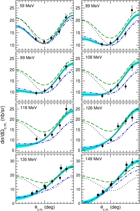
Figure 3: Angular dependence of the $\gamma p\to\gamma p$ differential cross-section in the center-of-mass system for a fixed photon-beam energies as specified for each panel. Data points are from SAL [25] — filled squares, and MAMI [27] — filled circles. The curves are: Klein-Nishina — dotted, Born graphs and WZW-anomaly — green dashed, adding the $p^{3}$ $\pi N$ loop contributions of B$\chi$PT — blue dash-dotted. The result of adding the $\Delta$ contributions, i.e., the complete NNLO result of Ref. [8], is shown by the red solid line with a band.

For now, however, I focus on the differences between the two $\chi$PT calculations. The earlier one [30] is done in HB$\chi$PT at order $p^{4}$. The latest is a manifestly-covariant calculation at order $p^{3}$ and $p^{4}/\varDelta$, hence includes the $\Delta$-isobar effects within the $\delta$-counting scheme. Despite the similar results for polarizabilities, the composition of these results order by order is quite different. In HB$\chi$PT one obtains for the central values (in units of $10^{-4}$fm³):

$$\alpha = \underbrace{12.2}_{\mathcal{O}(p^{3})}+\underbrace{(-0.1)}_{\mathcal{O}(p^{4})}=12.1\,,$$ (18)

$$\beta = \underbrace{1.2}_{\mathcal{O}(p^{3})}+\underbrace{2.2}_{\mathcal{O}(p^{4})}=3.4\,.$$ (19)

while in B$\chi$PT with $\Delta$’s:

$$\alpha = \underbrace{6.8}_{\mathcal{O}(p^{3})}+\underbrace{(-0.1)+4.1}_{\mathcal{O}(p^{4}/\varDelta)}=10.8\,,$$ (20)

$$\beta = \underbrace{-1.8}_{\mathcal{O}(p^{3})}+\underbrace{7.1-1.3}_{\mathcal{O}(p^{4}/\varDelta)}=4.0\,.$$ (21)

The difference at the leading order comes precisely due to the ‘higher-order’ terms. For instance, for the magnetic polarizability at $\mathcal{O}(p^{3})$, in one case we have:

$$\beta^{(3)HB}=\frac{e^{2}g_{A}^{2}}{768\pi^{2}f_{\pi}^{2}m_{\pi}}\,,$$ (22)

while in the other:

$$\beta^{(3)} = \frac{e^{2}g_{A}^{2}}{192\pi^{3}f_{\pi}^{2}M_{N}}\int\limits^{1}_{0}\!dx\,\bigg{\{}1-\frac{(1-x)(1-3x)^{2}+x}{\mu^{2}(1-x)+x^{2}}-\frac{x\mu^{2}+x^{2}[1-(1-x)(4-20x+21x^{2})]}{\big{[}\mu^{2}(1-x)+x^{2}\big{]}^{2}}\bigg{\}}$$ (23)

$$= \frac{e^{2}g_{A}^{2}}{192\pi^{3}f_{\pi}^{2}M_{N}}\Big{[}\,\frac{\pi}{4\mu}+18\ln\mu+\frac{63}{2}-\frac{981\pi}{32}\mu-\big{(}100\,\ln\mu+\frac{121}{6}\big{)}\mu^{2}+\ldots\Big{]}.$$

The first term in the expanded expression (23) is exactly the same as the HB result (22), but how about the higher-order terms. Their coefficients are at least a factor of 10 bigger than the coefficient of the leading term. Given that the expansion parameter is $\mu\sim 1/7$, there is simply no argument why these terms should be neglected.

As a consequence, the neat agreement of the HB $p^{3}$ result with the empirical numbers for $\alpha$ and $\beta$ should perhaps be viewed as a remarkable coincidence, rather than, as it’s often viewed, a “remarkable prediction” of HB$\chi$PT. In fact, the predictive power is what is first of all compromised by the unnaturally large, higher order (in HB-expansion) terms. These terms will of course be recovered in the higher-order HB calculations, but with each order higher there will be an increasingly higher number of unknown LECs. In contrast, the covariant results provide an example of how one gets to the important effects already in the lower-order calculations, before new LECs start to appear.

Now let’s return to the dispersion relations in the pion mass squared. Denoting $t=\mu^{2}$, the dispersion relation for the magnetic polarizability should read

$$\mathrm{Re}\,\beta(t)=-\frac{1}{\pi}\int\limits_{-\infty}^{0}dt^{\prime}\,\frac{\mathrm{Im}\,\beta(t^{\prime})}{t^{\prime}-t}\,.$$ (24)

The imaginary part at the 3rd order can be calculated from the first line of Eq. (23),

$$\mathrm{Im}\,\beta^{(3)}(t) = -\,C\,\,\mathrm{Im}\,\int\limits^{1}_{0}\!dx\,\bigg{\{}\frac{(1-x)(1-3x)^{2}+x+\mbox{$\frac{x}{1-x}$}}{(1-x)t+x^{2}-i\epsilon}$$

$$\hskip 113.81102pt-\frac{d}{dt}\frac{x\,t+x^{2}[1-(1-x)(4-20x+21x^{2})]}{(1-x)[(1-x)t+x^{2}-i\epsilon]}\bigg{\}}$$

$$= -\frac{\pi C}{8\lambda^{3}}\big{[}2-72\lambda+t(418\lambda-246)-t^{2}(316\lambda-471)+t^{3}(54\lambda-212)+27t^{4}\big{]},$$

where $C=\frac{e^{2}g_{A}^{2}}{192\pi^{3}f_{\pi}^{2}M_{N}}$ and $\lambda=\sqrt{-t\,(1-\mbox{\small{$\frac{1}{4}$}}t)}$. At this order there are no counter-terms, hence no subtractions, and indeed I have verified that the unsubtracted relation (24) gives exactly the same result as Eq. (23). The relation for the electric polarizability $\alpha$ has been verified in a similar fashion. These tests validate the analyticity assumption and elucidate the nature of the ’higher-order’ terms.

Finally, let me note that such dispersion relations, as well as the usual ones (in energy) [31], do not hold in the framework of Infrared Regularization (IR) [20]. The IR loop-integrals will always, in addition to the unitarity cuts, have an unphysical cut. Although the unphysical cut lies far from the region of $\chi$PT applicability and therefore does not pose a threat to unitarity, it does make an impact, and as result, a set of the higher-order terms is altered. To me, this is a showstopper. The only practical advantage of the manifest Lorentz-invariant formulation over the HB one is the account of ‘higher-order’ terms which may, or may not, be unnaturally large. Giving up on analyticity, one has no principle to assess these terms reliably.

5 Summary

Here are some points which have been illustrated in this paper:

• The region of applicability of B$\chi$PT without the $\Delta$(1232)-baryon is: $p\ll 300$ MeV. An explicit $\Delta(1232)$ is needed to extend this limit to substantially higher energies. Two schemes are presently used to power-count the $\Delta$ contributions: SSE and $\delta$-expansion.

• Inclusion of heavy fields poses a difficulty with power counting in a Lorentz-invariant formulation — contributions of lower- and higher-order arise in a calculations given-order graph. However, this is not a problem — the lower-order contributions renormalize the available LECs, while the higher-order ones are, in fact, required by analyticity and should be kept.

• Dispersion relations in the pion-mass squared have been derived and are shown to hold in the examples of lowest order chiral corrections to the nucleon mass and polarizabiltities.

• The present state-of-art $\chi$PT calculations of low-energy Compton scattering are in a good agreement with experimental cross-sections, but have an appreciable discrepancy with PDG values for proton polarizabilities.

References

- [1] S. Weinberg, Physica A 96, 327 (1979).
- [2] J. Gasser and H. Leutwyler, Annals Phys. 158 (1984) 142.
- [3] J. Gasser, M. E. Sainio and A. Svarc, Nucl. Phys. B 307, 779 (1988).
- [4] E. Jenkins and A. V. Manohar, Phys. Lett. B 259, 353 (1991).
- [5] E. Jenkins and A. V. Manohar, Phys. Lett. B 255, 558 (1991).
- [6] T. R. Hemmert, B. R. Holstein and J. Kambor, Phys. Lett. B 395, 89 (1997); J. Phys. G 24, 1831 (1998).
- [7] V. Pascalutsa and D. R. Phillips, Phys. Rev. C 67, 055202 (2003).
- [8] V. Lensky and V. Pascalutsa, Pisma Zh. Eksp. Teor. Fiz. 89, 127 (2009) [JETP Lett. 89, 108 (2009)]; arXiv:0907.0451 [hep-ph], submitted to Eur. J. Phys. C.
- [9] V. Pascalutsa and M. Vanderhaeghen, Phys. Rev. Lett. 95, 232001 (2005); Phys. Rev. D 73, 034003 (2006); Phys. Rev. Lett. 94, 102003 (2005); Phys. Rev. D 77, 014027 (2008); Phys. Lett. B 636, 31 (2006).
- [10] L. S. Geng, J. Martin Camalich, L. Alvarez-Ruso and M. J. Vicente Vacas, Phys. Rev. D 78, 014011 (2008).
- [11] L. S. Geng, J. Martin Camalich and M. J. Vicente Vacas, Phys. Lett. B 676, 63 (2009).
- [12] B. Long and U. van Kolck, arXiv:0907.4569 [hep-ph].
- [13] J. A. McGovern, H. W. Griesshammer, D. R. Phillips and D. Shukla, arXiv:0910.1184 [nucl-th].
- [14] K. Johnson and E. C. Sudarshan, Annals Phys. 13, 126 (1961).
- [15] G. Velo and D. Zwanziger, Phys. Rev. 186, 1337 (1969).
- [16] S. Deser, V. Pascalutsa and A. Waldron, Phys. Rev. D 62, 105031 (2000).
- [17] S. Weinberg and E. Witten, Phys. Lett. B 96, 59 (1980).
- [18] V. Pascalutsa, M. Vanderhaeghen and S. N. Yang, Phys. Rept. 437, 125 (2007).
- [19] H. Krebs, E. Epelbaum and U. G. Meissner, Phys. Rev. C 80, 028201 (2009); arXiv:0905.2744 [hep-th].
- [20] T. Becher and H. Leutwyler, Eur. Phys. J. C 9, 643 (1999).
- [21] J. Gegelia and G. Japaridze, Phys. Rev. D 60, 114038 (1999); J. Gegelia, G. Japaridze and X. Q. Wang, J. Phys. G 29, 2303 (2003).
- [22] B. R. Holstein, Comm. Nucl. Part. Phys. 20, 301 (1992); See also, B. R. Holstein, these proceedings.
- [23] F. J. Federspiel et al., Phys. Rev. Lett. 67, 1511 (1991).
- [24] A. Zieger, R. Van de Vyver, D. Christmann, A. De Graeve, C. Van den Abeele and B. Ziegler, Phys. Lett. B 278, 34 (1992).
- [25] E. L. Hallin et al., Phys. Rev. C 48, 1497 (1993).
- [26] B. E. MacGibbon, G. Garino, M. A. Lucas, A.M. Nathan, G. Feldman and B. Dolbilkin, Phys. Rev. C 52, 2097 (1995).
- [27] V. Olmos de Leon et al., Eur. Phys. J. A 10, 207 (2001).
- [28] D. Babusci, G. Giordano and G. Matone, Phys. Rev. C 57, 291 (1998).
- [29] W. M. Yao et al. [Particle Data Group], J. Phys. G 33, 1 (2006).
- [30] S. R. Beane, M. Malheiro, J. A. McGovern, D. R. Phillips and U. van Kolck, Phys. Lett. B 567, 200 (2003) [Erratum-ibid. B 607, 320 (2005)]; Nucl. Phys. A 747, 311 (2005).
- [31] B. R. Holstein, V. Pascalutsa and M. Vanderhaeghen, Phys. Rev. D 72, 094014 (2005).