Duality Argument for the Chiral-nematic Phase of Planar Spins

Abstract

A duality argument for the recently discovered chiral-nematic phase of the XY model in a triangular lattice is presented. We show that a new Ising variable naturally emerges in mapping the antiferromagnetic $J_{1}-J_{2}$ classical XY spin Hamiltonian onto an appropriate Villain model on a triangular lattice. The new variable is the chirality degree of freedom, which exists in addition to the usual vortex variables, in the dual picture. Elementary excitations and the associated phase transition of the Ising degrees of freedom are discussed in some detail.

I Introduction

A description of the excitations of a classical ferromagnet in a two-dimensional lattice is based on two entities: spin waves, which are small fluctuations of the spin orientation from their ground-state direction, and vortices, which are topological structures of spins carrying a non-zero winding number. Among the two, the latter excitation is more effective at destroying the coherence of spins and ultimately drives the phase transition between a quasi-long-range ordered (QLRO) phase and a disordered, paramagnetic phase KT . A convenient mathematical description of the phase transition in terms of the vortex variable is afforded by the mapping first discussed by Villain (Villain mapping) villain-map .

There are instances, however, where vortices do not exhaust all the relevant excitations for the phase transition. Another variable, namely, chirality, often appears in models of classical spins with frustration villain-chirality . With its symmetry being Ising-like, the chirality fluctuation can drive a second phase transition, apart from the one driven by vortex proliferation, of Ising universality class. A generalization of the Villain mapping for spin models with frustration was given by Villain villain-chirality , where it was demonstrated that the chirality emerges as a new, independent excitation mode of the model.

As a most recent example of a chirality-driven phase transition, it was shown in the context of a generalized antiferromagnetic XY spin model on a triangular lattice that there can be a chirality-driven phase transition taking place at temperatures well above the magnetic transition temperature PONH . The situation stands in contrast with the case of standard antiferromagnetic XY model on the same lattice, which only reveals a tiny separation between the chirality order ($T_{\chi})$ and the magnetic order ($T_{\mathrm{KT}}$) temperatures literature .

The aim of this paper is to place the observations made in Ref. PONH, in the context of the duality mapping of Villain by identifying the proper Ising variables associated with the chirality. While Villain’s original paper villain-chirality considered a square lattice, we focus here on a triangular lattice, as was the case for the numerical work of Ref. PONH, . A more elaborate discussion of Villain’s original model appeared in the work of Lee and Grinsteindhlee , but their discussion was for a square lattice, and the issue of the chirality did not arise in their work.

II Duality Mapping

The model studied in Ref. PONH, reads

$$H=J_{1}\sum_{\langle ij\rangle}\cos(\varphi_{ij})+J_{2}\sum_{\langle ij\rangle}\cos(2\varphi_{ij}),$$ (1)

where $\varphi_{ij}$ is the angle difference $\varphi_{i}-\varphi_{j}$ between nearest neighbors $\langle ij\rangle$. Focusing on a pair-wise interaction $J_{1}\cos[\varphi_{ij}]\!+\!J_{2}\cos[2\varphi_{ij}]$, the minimum energy angle for a given $\langle ij\rangle$ bond is two-fold degenerate at $\pi\pm\Delta$, $\Delta=\cos^{-1}(J_{1}/4J_{2})$, provided $4J_{2}>J_{1}$. For $4J_{2}<J_{1}$, a single minimum-energy angle is achieved, and the duality mapping proceeds in the same manner as in the ferromagnetic case.

An appropriate Villain model for the interaction having a double minima is given by the pairwise probability weight

$$P[\varphi_{ij}]=\sum_{n_{ij},t_{ij}}\exp\left(-{K\over 2}[\varphi_{ij}\!-\!\pi\!-\!\Delta t_{ij}\!+\!2\pi n_{ij}]^{2}\right).$$ (2)

We introduce two integer link fields: $n_{ij}$, which run from $-\infty$ to $\infty$, and $t_{ij}$, which takes on two values $t_{ij}=\pm 1$ corresponding to two equivalent minima. Both fields change sign under the interchange of the lattice indices, $n_{ji}=-n_{ij}$, and $t_{ji}=-t_{ij}$. $K$ is related to the inverse temperature $1/T$. Going through the standard Villain mapping gives an alternative expression containing only the first power of $\varphi_{ij}$:

$$P[\varphi_{ij}]=\sum_{l_{ij},t_{ij}}\exp\left(-{1\over 2K}l_{ij}^{2}+il_{ij}(\varphi_{ij}\!-\!\pi\!-\!\Delta t_{ij})\right),$$ (3)

where $l_{ij}$ is another integer field running from $-\infty$ to $\infty$. The partition function $Z$ is obtained as the product of $P[\varphi_{ij}]$’s over all nearest-neighbor links:

$$Z=\prod_{\langle ij\rangle}P[\varphi_{ij}]=\sum_{\{l_{ij},t_{ij}\}}\prod_{i}\left(\int_{-\infty}^{\infty}d\varphi_{i}\right)$$

$$\exp\left(-{1\over 2K}\sum_{\langle ij\rangle}l_{ij}^{2}+i\sum_{\langle ij\rangle}l_{ij}(\varphi_{ij}\!-\!\pi\!-\!\Delta t_{ij})\right).$$ (4)

The exponential factor in the above equation is evaluated for each configuration $\{l_{ij},t_{ij}\}$ and is summed over all possible configurations to give $Z$. Integration over the angle $\phi_{i}$ can be done first, which imposes current conservation at each site. In turn, the constraint can be solved by introducing a dual integer field $h_{I}$, which is connected to $l_{ij}$ by

$$l_{i,i+e_{1}} = h_{I}-h_{I+E_{1}},$$

$$l_{i,i-e_{3}} = h_{I+E_{3}}-h_{I},$$

$$l_{i,i+e_{2}} = h_{I-E_{2}+E_{3}}-h_{I+E_{3}},$$

$$i_{i,i-e_{1}} = h_{I+E_{1}-E_{2}+E_{3}}-h_{I-E_{2}+E_{3}},$$

$$i_{i,i+e_{3}} = h_{I+E_{1}-E_{2}}-h_{I+E_{1}-E_{2}+E_{3}},$$

$$i_{i,i-e_{2}} = h_{I+E_{1}}-h_{I+E_{1}-E_{2}}.$$ (5)

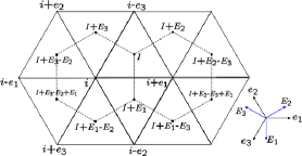
Figure 1: Representation of the original triangular lattice (full line) and the dual hexagonal lattice (dotted line) sites labeled by lower case and upper case letters, respectively. Nearest-neighbor vectors are denoted as $e_{1}$ ($E_{1}$) through $e_{3}$ ($E_{3}$) for the triangular (hexagonal) lattice.

See Fig. 1 for the definitions of various labels.

Now, we have the partition function

$$Z = \sum_{\{h_{I},t_{ij}\}}e^{-A},$$

$$A = {1\over 2K}\sum_{\langle IJ\rangle}(h_{I}\!-\!h_{J})^{2}+i\sum_{\langle IJ\rangle}(h_{I}\!-\!h_{J})(\pi\!+\!\Delta t_{ij}),$$

where $A$ is given as the sum over the dual links $\langle IJ\rangle$. The spin-wave contribution to $Z$ has been dropped. On re-organizing the expression on the far right of $A$ for each $h_{I}$, we get an equivalent expression

$$\sum_{\langle IJ\rangle}(h_{I}\!-\!h_{J})(\pi\!+\!\Delta t_{ij})=\sum_{I}h_{I}(3\pi+\Delta c_{I}).$$ (7)

Here, $c_{I}$ is the sum of the $t_{ij}$’s for each triangle centered at $I$ and going in the counter-clockwise sense. The allowed values of $c_{I}$ are $c_{I}=\pm 3,\pm 1$. The partition function is reduced to

$$Z\!=\!\sum_{\{h_{I},t_{ij}\}}\exp\left(-{1\over 2K}\sum_{\langle IJ\rangle}(h_{I}\!-\!h_{J})^{2}\!-\!i\sum_{I}h_{I}(\pi\!+\!\Delta c_{I})\right).$$ (8)

At this point, we invoke the Poisson sum formula to re-write the partition function as

$$Z=\sum_{\{m_{I},t_{ij}\}}\prod_{I}\left(\int_{-\infty}^{\infty}d\theta_{I}\right)$$

$$\exp\left(-{1\over 2K}\sum_{\langle IJ\rangle}(\theta_{I}-\theta_{J})^{2}+2\pi i\sum_{I}M_{I}\theta_{I}\right),$$

$$M_{I}=m_{I}-{1\over 2}-{\Delta\over 2\pi}c_{I}.$$ (9)

Here, $m_{I}$ is another integer field from $-\infty$ to $\infty$ defined at the dual sites $I$, which will play the role of the vorticity. We will integrate out $\theta_{I}$ to obtain the partition function solely in terms of the vorticity $m_{I}$ and chirality $c_{I}$:

$$Z\sim\sum_{\{m_{I},t_{ij}\}}\exp\left(-2\pi^{2}K\sum_{IJ}M_{I}G_{IJ}M_{J}\right).$$ (10)

In the sum, $I$ and $J$ independently run over all dual-lattice sites. The real-space Green’s function, $G_{IJ}$, is given by

$$G_{IJ}=a^{2}\int{{d^{2}{\bf k}}\over{(2\pi)}^{2}}{{e^{i{\bf k}\cdot{\bf r}_{IJ}}}\over{4-2\cos(k_{x}a)-2\cos(k_{y}a)}}.$$ (11)

It is convenient to use the regularized Green’s function $G^{\prime}_{IJ}$: $G^{\prime}_{IJ}=G_{IJ}-G_{{\bf 0}}$, so

$$Z=\sum_{\{m_{I},t_{ij}\}}\exp\left(-2\pi^{2}KG_{{\bf 0}}\left(\sum_{I}M_{I}\right)^{2}\right)$$

$$~{}~{}~{}~{}~{}\times\exp\left(-2\pi^{2}K\sum_{IJ}M_{I}G^{\prime}_{IJ}M_{J}\right).$$ (12)

Since $G_{{\bf 0}}\sim(1/2\pi)\ln(L/a)$, the allowed configurations are those with total vorticity $\sum_{I}M_{I}=0$. With the help of the result at large distances

$$G^{\prime}_{IJ}\sim-{1\over 2\pi}\ln{r_{IJ}\over a}-{1\over 4},$$ (13)

the partition function may be rewritten as

$$Z\!=\!\sum_{\{m_{I},t_{ij}\}}\exp\Bigl{(}-{\pi^{2}\over 2}K\sum_{I}M_{I}^{2}+\pi K\sum_{I\neq J}M_{I}M_{J}\ln\left|{r_{IJ}\over a}\right|\Bigr{)}.$$

We have used the relation $(\sum_{I}M_{I})^{2}=0=\sum_{I}M_{I}^{2}+\sum_{I\neq J}M_{I}M_{J}$. Often the fugacity term is defined by $y=\exp(-\pi^{2}K/2)$. This term controls the number of (total) vortices in the system. Equation (II) is the desired action expressed solely in terms of the vorticity $m_{I}$ and the chirality $c_{I}$ (or $t_{ij}$).

$c_{I}$	${1\over 2}+{1\over 4}(1-\delta)c_{I}$	$m_{I}$	$M_{I}$
3	${5\over 4}-{3\over 4}\delta$	1	$-{1\over 4}+{3\over 4}\delta$
-3	$-{1\over 4}+{3\over 4}\delta$	0	${1\over 4}-{3\over 4}\delta$
1	${3\over 4}-{1\over 4}\delta$	1	${1\over 4}+{1\over 4}\delta$
-1	${1\over 4}+{1\over 4}\delta$	0	$-{1\over 4}-{1\over 4}\delta$

Table 1: Local chirality $c_{I}$ and local vorticity $m_{I}$ for which the net vorticity $M_{I}$ is least costly.

In Ref. PONH, , the large $J_{2}/J_{1}$ region was shown to have a chirality ordering transition taking place well above the magnetic transition. In the $J_{2}/J_{1}\gg 1$ region, $\Delta=\cos^{-1}(J_{1}/4J_{2})$ becomes close to $\pi/2$, and one can write $\Delta=\pi(1-\delta)/2$, where $\delta$ is given by $\sin(\pi\delta/2)=J_{1}/4J_{2}$. The fugacity consideration requires that $M_{I}^{2}$ be as small as possible at low temperatures, and in Table 1, the smallest net vorticity $M_{I}$ for each chirality value $c_{I}$ is shown. Furthermore, $M_{I}^{2}$ for $c_{I}=\pm 3$ is less than $M_{I}^{2}$ when $c_{I}=\pm 1$,

$$M_{I}^{2}(c_{I}=\pm 3)-M_{I}^{2}(c_{I}=\pm 1)\approx-\delta/2<0.$$ (15)

The global minimum of $\sum_{I}M_{I}^{2}$ is obtained if each triangle carries the chirality $c_{I}=\pm 3$. In practice, this is possible by arranging all the up triangles to carry $c_{I}=3$ and all the down triangles to carry $c_{I}=-3$, or vice versa. This is the chirality-ordered phase at low temperature.

The cheapest excitation is the one with the least increase in $M_{I}^{2}$. Such an excitation is achieved if for a given triangle, two of the $t_{ij}$’s reverse their directions, and $c_{I}=3$ becomes $c_{I}=-1$ or $c_{I}=-3$ becomes $c_{I}=1$. As one can see from Table 1, the corresponding change in the net vorticity is from $M_{I}=-1/4+3\delta/4$ to $M_{I}=-1/4-\delta/4$, or $\Delta M_{I}=-\delta$. Similarly $c_{I}=-3\rightarrow 1$ incurs the change $\Delta M_{I}=\delta$. Such excitations are called incommensurate vortices incomm-vortex to set them apart from integer changes in the vorticity, also called commensurate vortices. At a temperature $T_{I}$ that scales with $\delta$, we thus expect an Ising transition caused by the proliferation of incommensurate vortices. Imagine we draw a line segment from $I$ and $J$ that intersects the $\langle ij\rangle$ bond with its $t_{ij}$ reversed. Then as one can see from Fig. 2, the creation of incommensurate vortices is achieved if the line segments close onto themselves, forming closed loops. In the dual hexagonal lattice, the smallest such loop would be a single hexagon. At the Ising transition, the size of the closed loop diverges. In the numerical study of Eq. (1), an Ising transition with $T_{I}\sim\delta$ was identified for the large $J_{2}/J_{1}$ region.

A flip of a single $t_{ij}$ in a triangle, on the other hand, changes $c_{I}=3$ (-3) to $c_{I}=1$ (-1), and the net vorticity change $\Delta M_{I}=\pm(1/2-\delta/2)$. Close to $\delta=0$, this is creating an isolated half-integer vortex with a rather high energy cost. To avoid the creation of a half-integer vortex, all triangles must have $\Delta c_{I}=\pm 4$, rather than $\Delta c_{I}=\pm 2$. For an open line segment, if both ends of the line terminate at the A or the B sublattice sites of the hexagonal lattice, the endpoints are associated with half-integer vortices of the same sign. If one end terminates on a sublattice different from that of the other end, then one has created a pair of half-integer vortices of opposite charges. It is then the proliferation of closed loops in the dual hexagonal space that corresponds to the Ising transition of the chirality. At exactly $\delta=0$ ($J_{1}=0$), the energy cost for the flip of chirality by four units becomes zero, so already at zero temperature, one has a disordered chirality phase. At small $\delta$, a proliferation of the cluster of triangles with $\Delta c_{I}=\pm 4$ or a proliferation of closed loops in the dual hexagonal space occurs at a small finite temperature $T_{I}$. On the other hand, once the length of the line becomes infinitely long, the half-integer vortices becomes free, and the half-integer vortex pairs unbind. This is the KT transition of half-integer vortices at a higher temperature $T_{\mathrm{KT}}$.

III Summary

To summarize, we have presented a duality argument for the antiferromagnetic $J_{1}-J_{2}$ XY spin model on a triangular lattice. In carrying out the Villain mapping of the original spin model, an additional Ising degree of freedom emerges naturally. This new degree of freedom corresponds to the spin chirality, and its excitation is responsible for the chirality phase transition of Ising universality. The natures of various possible Ising excitations are clarified in the dual model.

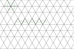
Figure 2: The thin lines forming the triangular lattice have the chirality $c_{I}=3$ for upward triangles and $c_{I}=-3$ for downward triangles. The thick lines have the local chirality $t_{ij}$ reversed from its ground state value, forming “defect bonds.” The lines (green dotted) that intersect such defect bonds can form a closed loop (the smallest such loop is a hexagon) or an open segment. Each point of the line segment carries vorticity changes of $\pm\delta$ if it is connected on both sides and $\pm(1/2-\delta/2)$ if it is connected on one side only.

References

• (1) J. M. Kosterlitz and D. J. Thouless, J. Phys. C: Solid State Phys. 6, 1181 (1973).
• (2) J. Villain, J. Physique 36, 581 (1975).
• (3) J. Villain, J. Phys. C: Solid State Phys. 10, 4793 (1977).
• (4) Jin-Hong Park, Shigeki Onoda, Naoto Nagaosa, and Jung Hoon Han, Phys. Rev. Lett. 101, 167202 (2008).
• (5) P. Olsson, Phys. Rev. Lett. 75, 2758 (1995); S. Lee and K.-C. Lee, Phys. Rev. B 57, 8472 (1998); S. E. Korshunov, Phys. Rev. Lett. 88, 167007 (2002); M. Hasenbusch, A. Pelissetto, and E. Vicari, J. Stat. Mech.: Theory Exp., P12002 (2005).
• (6) D. H. Lee and G. Grinstein, Phys. Rev. Lett. 55, 541 (1985).
• (7) D. H. Lee, G. Grinstein, and J. Toner, Phys. Rev. Lett. 56, 2318 (1986).
Refer to caption