On Formation Of A Shock Wave In Front Of A Coronal Mass Ejection With Velocity Exceeding The Critical One

Abstract

New study confirms conclusions made in [6]; according to it, there is a disturbed region expended along the CME propagation direction in front of a coronal mass ejection whose velocity $u$ is lower than the critical $u_{C}$ relative to the surrounding coronal plasma. The time difference brightness (plasma density) in the disturbed region smoothly decreases to larger distances in front of CME. A shock wave forms at u higher than $u_{C}$ in the front part of the disturbed region manifested as a discontinuity in radial distributions of the difference brightness.

1 Introduction

A coronal mass ejection (CME) structure in white light is often characterized by the following well-known features: a bright frontal structure (FS) that covers the region of decreased plasma density (cavity) that may includes a bright interior (core). However, besides the said features, another extended disturbed region defined by [4] can exist immediately in front of a CME. The aim of our study is to investigate changes in the disturbed region form, when a CME velocity increases, and possibilities for formation of a shock wave in this case.

2 Method of analysis

In the analysis, corona images obtained with the SOHO/LASCO C2 and C3 [1] were represented as the difference brightness $\Delta P=P(t)-P(t_{0})$, where $P(t_{0})$ is the undisturbed brightness at $t_{0}$ before the event considered, $P(t)$ is the disturbed brightness at any instant $t>t_{0}$. Calibrated LASCO images were used with the total brightness $P(t)$ expressed in units of the mean solar brightness (P_msb).

Images of the difference brightness were employed to investigate the CME dynamics and disturbed region. For the purpose we used presentations in the form of isolines and sections both along the solar radius at fixed position angles $PA$ and non-radial sections at various instants $t$. On all the images, the position angle $PA$ was calculated counterclockwise from the Sun’s north pole.

3 Data analysis

First we consider two CMEs (CME1 and CME2) whose velocities $V$ differ greatly at $R=$ 4-5 R_⊙ (R_⊙ is the solar radius). Two top panels of Figure 1 show the typical difference brightness form (in isolines) for these two CMEs at the instants, when their frontal structures FS appear in the C2 field of view. Figure 1a presents the slow CME1 (5 May 1997, $V\approx 400$ km s^-1), Figure 1c the fast CME2 (20 September 1997, $V\approx 800$ km s^-1). The values of velocity $V$ correspond to the linear fit of the height-time measurements for the fastest frontal parts of the CMEs and were taken from the CME catalogue (http://cdaw.gsfc.nasa.gov/CME˙list/).

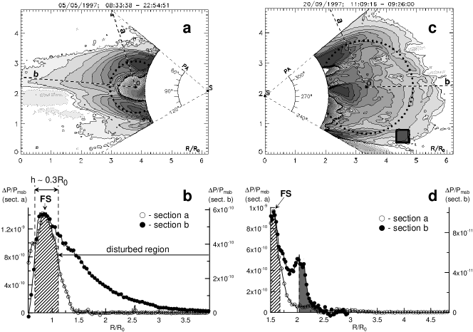
Figure 1: a, b – the slow CME1 on 5 May 1997; c, d – the fast CME2 on 20 September 1997; top panels (a, c) display images of the difference brightness in the form of isolines; the bottom panels (b, d) present distributions of the difference brightness depending on the distance $r$, measured from the frontal structure center (point O) along two different sections “a” and “b”, whose directions are shown on the top panels.

Figures 1a,b show that on the images of both CMEs the frontal structure FS can approximately be presented by a part of a circle with its center at O (dots on the figures). The main direction of the CME propagation that roughly coincides with its symmetry axis is indicated by a heavy dashed line “b”. It passes along the streamer belt or streamer chains [3, 5]; i.e., it is in the region of the quasistationary slow solar wind (SW).

In order to find the left boundary of the disturbed region (from the CME side), by analogy with [10] we determine the FS width $h$ as a width at a half-height of the difference brightness $\Delta P(r)$ distribution constructed from the FS center. For CME1, the frontal structure in the direction of section “a” (Figure 1a) is least distorted by the disturbed region effect and has a minimum width $h\approx 0.3$ R_⊙ (a curve with light circles in Figure 1b). Let us take the FS right-hand boundary as the left-hand boundary of the disturbed region, as shown in Figure 1b. Its position is indicated by a vertical dashed line. In Figure 1b, a curve with solid circles shows the $\Delta P(r)$ distribution along the section “b” in the direction of the CME propagation. The disturbed region is marked by a horizontal line with an arrow-head and labeled respectively.

The comparison between CME1 (slow) and CME2 (fast) yields two principal distinctions:

1. The isolines that correspond to the minimum difference brightness of the slow CME1 are extended along the direction of its propagation, while those of the fast one are close in form to a circle.

2. The difference brightness $\Delta P(r)$ distribution along the direction of the CME propagation continuously decreases up to the most specific front part of the disturbed region for the slow CME, whereas in the front part of the fast CME disturbed region a discontinuity appears in the $\Delta P(r)$ distribution on a scale $\delta_{F}\approx$ 0.2-0.3 R_⊙ (shaded in Figure 1d).

The $\Delta P(r)$ distributions constructed along the direction of the CME propagation are presented for the set of eight CMEs in Figure 2. CME velocities are different and increase from bottom to top in Figure 2, thus the slowest CME with $V\approx 230$ km s^-1 is shown on the bottom panel, and the fastest one with $V\approx 2000$ km s^-1 on the top panel.

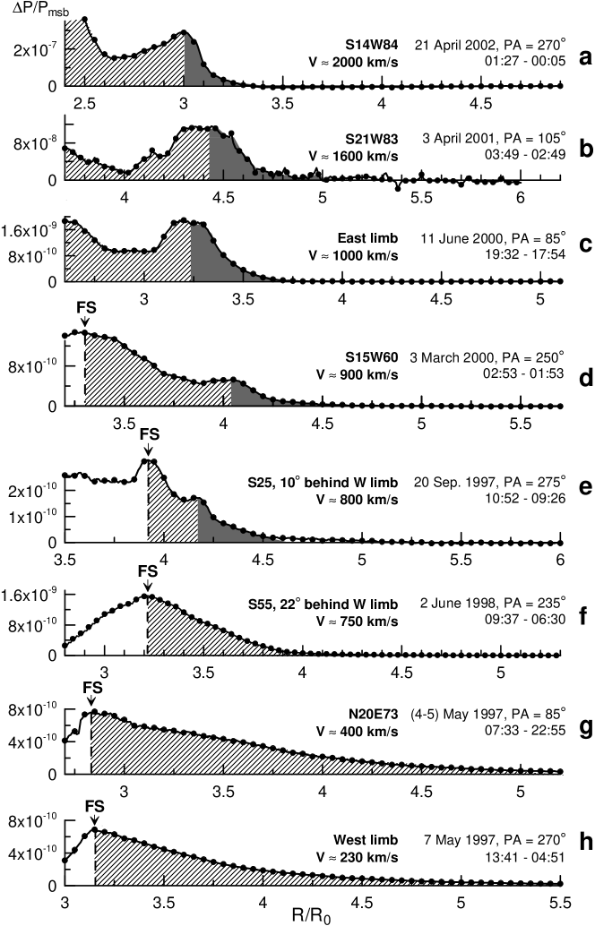
Figure 2: The $\Delta P(R)$ distributions for 8 CMEs along the direction of their propagation.

Slanted hatching in Figure 2 a-h presents the disturbed region and half of the frontal structure (labeled as FS). As the CME velocity increases from minimum ($V\approx 230$ km s^-1) to critical one $V_{C}\approx$ 750-800 km s^-1, width of the hatched region tends to decrease. Discontinuity in $\Delta P(R)$ distributions at the front boundary of the disturbed region (shaded parts in Figure 2 a-e) is observed when CME velocities $V$ are higher than the critical velocity $V_{C}$. At the same time at $V<V_{C}$ such discontinuity is absent, and the difference brightness distribution smoothly decreases with increasing distance until it becomes indistinguishable. Notice that CMEs with velocities $V$ close to the critical velocity VC (Figure 2 d-g) propagate near the plane of the sky; thus, their measured velocity is close to the real one (Figure 2 shows coordinates of places of the CME initiation on the solar disk, taken from [2] and Solar-Geophysical Data (http://sgd.ngdc.noaa.gov). Appearance of such a discontinuity at the front boundary of the disturbed region at $V>V_{C}$ was first described in [6].

Obviously, in processes of the “CME – undisturbed coronal plasma” interaction a crucial role should be played not by a $V$ value, but a value of CME velocity relative to the surrounding SW stream $u=V-V_{SW}$. Since CME velocities were determined in the direction of their propagation, we took a velocity of the slow SW flowing for the most part in the region of the coronal streamer belt and streamer chains, along which the majority of CMEs move, as the velocity $V_{SW}$ of the undisturbed solar wind [8].

Figure 3 presents values of the relative velocity $u$ measured for twenty four different CMEs at different distances. For $V_{SW}(R)$ we employed dependence derived by [12] of the slow SW velocity on the distance $R$ in the streamer belt. This dependence is shown by a dash-dot line in Figure 3.

Figure 3: CME velocities $u=V-V_{SW}$ relative to the surrounding SW depending on a distance from the solar center for the CME without discontinuity (open marks) and the CME with discontinuity (solid marks). The dash-dot curve indicates the velocity $V_{SW}$ of the quasistationary slow SW in the streamer belt from [12]. The dash curve shows the Alfven velocity in the streamer belt from [9].

In Figure 3, solid marks correspond to the CMEs having a discontinuity in the difference brightness distributions in front of the disturbed region. CME velocities $V$ were determined from the discontinuity motion. Open marks in Figure 3 indicate the CME without discontinuity. In this case we took a velocity from the CME catalogue (http://cdaw.gsfc.nasa.gov/CMElist/). Figure 3 shows that the cases with the discontinuity observed are in the high-velocity region, and the cases without discontinuity (the disturbed region smoothly decreased with distance is observed there) are for the most part in the low-velocity region. Hence we can assume that the discontinuity forms, when the relative CME velocity $u$ exceed some critical $u_{C}$ value. A critical velocity value may depend on a distance $R$.

Compare the obtained $u_{C}$ value with the typical velocity of disturbance propagation in the magnetized corona plasma that is roughly equal to the fast-mode MHD velocity $V_{MS}$ in the plasma. In order to estimate $V_{MS}$ at these distances we may use $V_{A}$ assuming that $V_{MS}\approx V_{A}$. Dashed line in Figure 3 indicates the $V_{A}(R)$ dependence obtained by [9].

Obviously in Figure 3 the Alfven velocity passes approximately between clusters of points, which apply to the CMEs with discontinuity and without it. Hence $u_{C}\approx V_{A}$, i.e., the desired critical velocity is roughly equal to the typical velocity of disturbance propagation in the magnetized plasma.

Hence we have a situation the classical gas dynamics refers to as “transonic transition” and formation of a shock wave. It was predicted theoretically, but it is first observed experimentally in the magnetized plasma.

4 On possibility for resolution of a shock front width

Here we will briefly discuss the problem of a possibility for resolution of a shock front width in the corona. The discontinuity is observed in distributions of the difference brightness $\Delta P(R)$ that results from free-electron scattering and is averaged along the line of sight in the optically thin corona. Since we do not know exactly the matter-density distribution along the line of sight, the observable scale $\delta_{F}$ in $\Delta P(R)$ distributions may differ from a real scale $\delta_{N}$ of the plasma density discontinuity. As a result of the averaging the observable discontinuity in the difference brightness profile can have larger scale than the real discontinuity in the density profile has.

In order to estimate an effect of such averaging, $\delta_{F}/\delta_{N}$ ratios were found in the context of a simple geometrical shock-front model in [6]. In the model considered, the shock-wave front was represented as a spherical shell with an outer radius $R_{F}$; the center of the shell was in the plane of the sky at $R_{C}$ from the solar center (these parameters were specified according to the CME form).

The brightness distribution $\Delta P(R)$, induced by free-electron scattering within the shell in the range from the shell center to its front edge, was calculated. At the given distance $R$, the brightness value is defined by the integral along the line of sight:

$$\Delta P(R)=\int\limits_{l}i(R,\theta)N(r)dl$$ (1)

where $i(R,\theta)$ is the brightness induced by the one-electron scattering, $N(r)$ – density. The $i(R,\theta)$ function depends on a impact distance $R$ and an angle $\theta$ relative to the plane of the sky. In the spherical shell, the density was supposed to change only depending on the distance $r$ from the sphere center. In each case we chose a density profile $N(r)$ such that a model brightness profile $\Delta P(R)$ obtained from $N(r)$ by integration of Equation (1) showed the best correlation with the experimental profile of the difference brightness $\Delta P(R)$. Then a scale $\delta_{N}$ of the plasma density discontinuity was found from the density profile $N(r)$ obtained.

Calculations show that the $\Delta P(R)$ profile broadening does not exceed 20% in comparison with the density profile $N(r)$. Thus, scale of a brightness profile discontinuity is a good approximation for determining scale of a density discontinuity in a shock wave front.

It is worth noting that, at $R\geq 10$ R_⊙, a new discontinuity (with thickness $\delta_{F}^{*}\ll\delta_{F}$) is observed to form in the anterior part of the shock front for events with $V>V_{C}$ considered above. Within the experimental error, thickness $\delta_{F}^{*}\approx$ 0.1-0.2 R_⊙ does not vary with distance and is determined by the LASCO C3 instrument spatial resolution. Transfer from the shock front with thickness $\delta_{F}$ to the discontinuity with thickness $\delta_{F}^{*}\ll\delta_{F}$ can be interpreted as transition from the collisional to collisionless shock wave [7]. Similar discontinuities in brightness profiles associated with collisionless shock waves were registered ahead fast halo-type CMEs ($V>1500$ km s^-1) at distances $>10$ R_⊙ in [11].

5 Conclusions

It has been shown that in front of a coronal mass ejection having a velocity $u$ lower than the critical $u_{C}$ relative to the surrounding coronal plasma there is a disturbed region expended along a direction of the CME propagation. The time difference brightness $\Delta P$ in the disturbed region smoothly decreases up to larger distances in front of the CME. Given $u>u_{C}$, a discontinuity forms in distribution of difference brightness or plasma density in the disturbed region front part. Since the $u_{C}$ value is close to the local fast-mode MHD velocity, which in corona approximately equal to the Alfven one, the formation of such a discontinuity when $u_{C}$ is exceeded may be identified with the formation of a shock wave.

Acknowledgments

The work was supported by program No. 16 part 3 of the Presidium of the Russian Academy of Sciences, program of state support for leading scientific schools NS-2258.2008.2, and the Russian Foundation for Basic Research (Project No. 09-02-00165a). The SOHO/LASCO data used here are produced by a consortium of the Naval Research Laboratory (USA), Max-Planck-Institut fuer Aeronomie (Germany), Laboratoire d’Astronomie (France), and the University of Birmingham (UK). SOHO is a project of international cooperation between ESA and NASA. The Mark 4 data are courtesy of the High Altitude Observatory/NCAR.

References

- [1] G. E. Brueckner, et al., Solar Phys. 162, 357–402 (1995).
- [2] H. Cremades, and V. Bothmer, Astronomy and Astrophysics 422, 307–322 (2004).
- [3] V. G. Eselevich, V. G. Fainshtein, and G. V. Rudenko, Solar Phys. 188, 277–297 (1999).
- [4] M. V. Eselevich, and V. G. Eselevich, Astronomy Reports 51, 947–954 (2007).
- [5] M. V. Eselevich, V. G. Eselevich, and K. Fujiki, Solar Phys. 240, 135–151 (2007).
- [6] M. Eselevich, and V. Eselevich, GRL 35, L22105 (2008).
- [7] M. Eselevich, and V. Eselevich, arXiv:0907.5245v1, (2009).
- [8] A. J. Hundhausen, JGR 98, 13177–13200 (1993).
- [9] G. Mann, H. Aurass, A. Klassen, C. Estel, and B. J. Thompson, “Coronal transient waves and coronal shock waves,” in 8th SOHO Workshop: Plasma Dynamics and Diagnostics in the Solar Transition Region and Corona, edited by J.-C. Vial and B. Kaldeich-Schumann, Proceedings of the Conference ESA SP-446, 1999, pp. 477–481.
- [10] T. Ch. Mouschovias, and A. I. Poland, Astrophys. J. 220, 675–682 (1978).
- [11] V. Ontiveros, and A. Vourlidas, Astrophys. J. 693, 267–275 (2009).
- [12] Y.-M. Wang, N. R. Jr. Sheeley, D. G. Socker, R. A. Howard, and N. B. Rich, JGR 105, 25133–25142 (2000).