Flow instabilities of magnetic flux tubes

Abstract

Context. Flow-induced instabilities of magnetic flux tubes are relevant to the storage of magnetic flux in the interiors of stars with outer convection zones. The stability of magnetic fields in stellar interiors is of importance to the generation and transport of solar and stellar magnetic fields.

Aims. We consider the effects of material flows on the dynamics of toroidal magnetic flux tubes located close to the base of the solar convection zone, initially within the overshoot region. The problem is to find the physical conditions in which magnetic flux can be stored for periods comparable to the dynamo amplification time, which is of the order of a few years.

Methods. We carry out nonlinear numerical simulations to investigate the stability and dynamics of thin flux tubes subject to perpendicular and longitudinal flows. We compare the simulations with the results of simplified analytical approximations.

Results. The longitudinal flow instability induced by the aerodynamic drag force is nonlinear in the sense that the growth rate depends on the perturbation amplitude. This result is consistent with the predictions of linear theory. Numerical simulations without friction show that nonlinear Parker instability can be triggered below the linear threshold of the field strength, when the difference in superadiabaticity along the tube is sufficiently large. A localised downflow acting on a toroidal tube in the overshoot region leads to instability depending on the parameters describing the flow, as well as the magnetic field strength. We determined ranges of the flow parameters for which a linearly Parker-stable magnetic flux tube is stored in the middle of the overshoot region for a period comparable to the dynamo amplification time.

Conclusions. The longitudinal flow instability driven by frictional interaction of a flux tube with its surroundings is relevant to determining the storage time of magnetic flux in the solar overshoot region. The residence time for magnetic flux tubes with $2\times 10^{21}$Mx in the convective overshoot layer is comparable to the dynamo amplification time, provided that the average speed and the duration of the downflow do not exceed about 50 m s ^-1 and 100 days, respectively, and that the lateral extension of the flow is smaller than about $10^{\circ}$.

1 Introduction

Observations of large solar active regions are indicative of an organised subsurface magnetic field along the azimuthal (east-west) direction, with opposite polarity orientations (from east to west or vice versa) in the northern and southern hemispheres. Emerging magnetic structures are in a filamentary state, in the form of magnetic flux concentrations (flux tubes) of various sizes (e.g., sunspots, pores). Flux tubes rise in the convection zone, emerge at the surface, and form bipolar magnetic regions, which follow polarity rules (Hale’s law) and systematic tilt angles (Joy’s law).

Theoretical studies indicate that weak magnetic fields are transported by flux expulsion (Schüssler 1984) and convective pumping (Tobias et al. 2001) to the lower boundary of the convection zone, where the toroidal magnetic field is amplified by radial and latitudinal velocity shear in the solar tachocline (see e.g., Solanki et al. 2006). The stably stratified lower convection zone, in particular the convective overshoot layer, is a likely location for the generation and storage of the large-scale azimuthal magnetic flux. Numerical studies simulating a layer of horizontal magnetic field in the bottom of the solar convection zone indicate that an initially uniform field underlying a field-free layer leads to the formation of magnetic flux tubes by magnetic Rayleigh-Taylor instability (e.g., Fan 2001). Following its formation, a toroidal magnetic flux tube can reach a mechanical equilibrium close to the bottom of the convection zone (Moreno-Insertis et al. 1992). The emergence of magnetic flux tubes driven by magnetic buoyancy and the properties of active regions (low-latitude emergence, tilt angles, proper motions of sunspots) require azimuthal flux densities of the order of $10^{5}$ G in the overshoot region (D’Silva & Choudhuri 1993; Fan et al. 1994; Caligari et al. 1995; Schüssler 1996). The possibilities for the generation of these flux densities have been reviewed by Schüssler & Rempel (2002), Schüssler & Ferriz-Mas (2003), and Ferriz-Mas & Steiner (2007).

The average duration of the solar activity cycle is about 11 years and the total magnetic flux emerging within one cycle ranges between orders of $10^{24}-10^{25}$ Mx. The amplification of the toroidal magnetic field to its maximum strength in about half an activity cycle raises the following question: how can the toroidal flux be stored stably for at least a few years in the dynamo amplification region? A related problem concerns the feedback of magnetic flux loss on the rate of toroidal flux generation. To more clearly understand magnetic flux generation and storage in the convective overshoot region, it is important to determine and constrain the effects of flows on the stability and dynamics of magnetic flux tubes. Here, we focus on: (a) the nonlinear development of flow-induced flux tube instabilities, which can be dynamically significant in the course of toroidal field amplification; and (b) effects of perpendicular flows on the storage of toroidal flux tubes. Consequently, some of the flow properties prevailing in the overshoot region can also be constrained, by requiring that flux tubes with field strengths of up to a few times $10^{4}$ G are stored in the overshoot region for about a few years.

We consider the possibility that the friction-induced instability (Holzwarth et al. 2007; Holzwarth 2008) leads to flux loss from the overshoot layer for field strengths below the Parker instability limit. We refer to such Parker-stable flux tubes as “sub-critical” throughout the paper. We investigate effects of flows on magnetic flux tubes in mechanical equilibrium to obtain quantitative estimates, and to answer the following question: how strongly do ($i$) finite-amplitude perturbations of flux tubes by perpendicular flows (see also Schüssler & Ferriz Mas 2007, paper I) and ($ii$) the frictional interaction of the tube with its surroundings limit the residence time of flux tubes in the overshoot region?

We approach the problem by considering the nonlinearity of friction-induced instability (Sect. 2), including a discussion of the effects of finite perturbations on the magnetic buoyancy instability (Sect. 2.3), and determine the ranges of flow parameters that allow the storage of sub-critical flux tubes subject to radial flows (Sect. 3).

The analyses and simulations were carried out in the framework of the thin flux tube approximation (Spruit 1981), which at present is the only existing approach that can deal with the small magnetically induced variations in density, pressure, and temperature corresponding to the high plasma $\beta$ ($>10^{5}$) of the deep solar convection zone.

2 Friction-induced instabilities

The mechanical equilibrium of a toroidal flux tube in the solar convection zone requires that the plasma within the tube rotates faster than the surrounding medium. Moreno-Insertis et al. (1992) demonstrated that a toroidal flux tube rotating initially at the same rate as the external medium can reach this equilibrium by developing an internal prograde flow. The speed of this “equilibrium” flow depends on the magnetic field strength, depth, and latitude. A flux tube subject to non-axisymmetric perturbations (varying in azimuth) will develop MHD waves that propagate in prograde and retrograde directions. If the internal flow speed (in the rest-frame of the external medium) is greater than the phase speed of the slowest transversal retrograde wave mode, this wave mode will be advected in the prograde direction, while being amplified (Holzwarth et al. 2007, hereafter paper II). The critical flux density for the instability is lower than that of the Parker instability. Holzwarth (2008, hereafter paper III) extended the analysis in paper II to toroidal flux tubes, thus including the effect of magnetic curvature force and rotation.

The linear analyses in papers II and III considered Stokes-type friction, which is linear in perpendicular velocity. To test the results of the linear stability analysis in the nonlinear context, we shall consider the drag force, which is quadratic in velocity. This test can be implemented by carrying out fully nonlinear numerical simulations of flux tubes subject to non-axisymmetric perturbations.

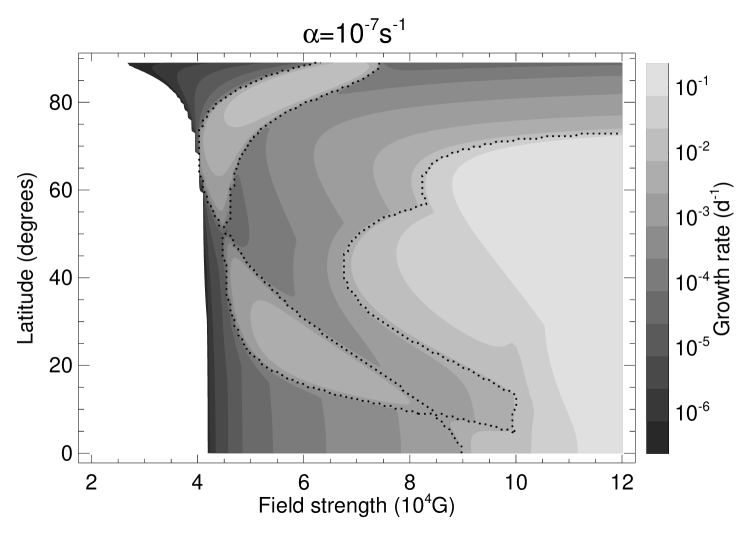
Figure 1: Stability diagram for toroidal flux tubes located in the middle of the solar overshoot region. The shaded areas indicate unstable configurations with the grey scale representing the growth rate. Dotted lines outline regions of Parker instability.

2.1 Linear results

The hydrodynamic drag force exerted by a steady flow with velocity ${\bf v}_{\perp}$ perpendicular to a straight cylinder is given by

$${\bf F}_{\rm D}=-C_{\rm D}\frac{\rho_{e0}\varv_{\perp}{\bf v}_{\perp}}{\pi R_{\rm t}},$$ (1)

where $C_{D}$ is the drag coefficient, $\rho_{e0}$ is the density of the external medium neighbouring the equilibrium flux tube, and $R_{\rm t}$ is the cross-sectional radius of the equilibrium tube.

The Stokes-type friction force per unit volume,

$${\bf F}_{\rm St}=-\alpha\rho_{e0}{\bf v}_{\perp},$$ (2)

where the constant $\alpha$ is the friction coefficient, was considered in papers II and III to include the friction-type deceleration in the linearised equation of motion. In paper II it was shown that the critical field strength for friction-induced instability hardly depends on the value of $\alpha$. Comparing Eq. (2) with Eq. (1), one finds that the friction coefficient is of the order

$$\alpha\sim\frac{\varv_{\perp}}{\pi R_{\rm t}},$$ (3)

where the drag coefficient, $C_{\rm D}$, is set to be unity, because of the cylindrical cross-section and high Reynolds number (Batchelor 1967).

We consider a toroidal flux tube located in the convective overshoot region, parallel to the equatorial plane. For the stratification of the ambient medium, we use a model convection zone developed by Skaley & Stix (1991), which uses a non-local treatment of convection as described by Shaviv & Salpeter (1973). In the model, the overshoot region extends about $10^{4}$ km below the base of the convection zone, which is defined as the depth at which the convective energy flux changes its sign, at about $r=512$ Mm. The thickness of the overshoot layer corresponds to about 20% of the local pressure scale height. Throughout the paper, the terms bottom, middle, and top (levels) of the overshoot region are used to refer to the radial positions at, respectively, 2000, 5000, and 8000 km above the lower boundary of the overshoot region, which is at a radius of $r=502$ Mm ($\sim 0.72R_{\odot}$).

The linear stability analysis of paper III has provided growth rates of the friction-induced instability for toroidal flux tubes. In Fig. 1, growth rates are shown as a function of the field strength ($B_{0}$) and latitude ($\lambda_{0}$) located in the middle of the overshoot region, for $\alpha=10^{-7}$ s^-1 and rigid solar rotation. In paper III, the value of $\alpha$ was chosen by determining the average perpendicular velocity of the mass elements of the flux tube during the initial stages of nonlinear numerical simulations for a flux tube with $\Phi\simeq 3\times 10^{21}$ Mx. The friction-induced instability sets in for $B_{0}\gtrsim 4\times 10^{4}$ G. The onset of Parker instability is in the interval $6\times 10^{4}\lesssim B_{0}\lesssim 10^{5}$ G at low latitudes.

2.2 Nonlinear simulations

We carried out numerical simulations of a toroidal flux tube using a semi-implicit finite-difference scheme developed by Moreno-Insertis (1986), that was extended to three dimensions and spherical geometry by Caligari et al. (1995). The numerical procedure is based on the equations of ideal magnetohydrodynamics in the framework of the thin flux tube approximation (Spruit 1981), in the form given by Ferriz-Mas & Schüssler (1993, 1995). In the numerical scheme, the flux tube is described by a string of Lagrangian mass elements, which move in three dimensions under the effects of various body forces. The equation of motion for the material inside the toroidal flux tube, in a reference frame rotating with the angular velocity of the tube, ${\bf\Omega}$, is written as

$$\rho_{i}\frac{D{\bf v}_{i}}{Dt} = -\nabla\Big{(}p_{i}+\frac{B^{2}}{8\pi}\Big{)}+\frac{({\bf B\cdot\nabla}){\bf B}}{4\pi}$$ (4)

$$+\rho_{i}\big{[}{\bf g-\Omega\times(\Omega\times r)}\big{]}+2\rho_{i}{\bf v}_{i}{\bf\times\Omega}+{\bf F}_{\rm D},$$

where $D/Dt\equiv\partial/\partial t+{\bf v}\cdot\nabla$ is the Lagrangian derivative, the subscript $i$ denotes quantities inside the flux tube (the subscript $e$ denotes external quantities in the following). The terms on the right hand side of the equation are, respectively, the total pressure force (gas and magnetic), magnetic tension force, effective gravity (including the centrifugal force), Coriolis force, and the hydrodynamic drag force, which is given by Eq. (1). We assume rigid rotation in the solar interior. Although rotational velocity shear can be incorporated into the framework of our model (Ferriz-Mas & Schüssler 1995; Caligari et al. 1995), we disregard it for the sake of clarity, to focus on the fundamental effects of radial flows on flux tube dynamics. Caligari et al. (1995) found that external shear does not have a significant effect on the stability properties and dynamics of flux tubes in the Sun.

Figure 2: Comparison of the analytical solutions for the growth rate of the friction-induced instability (lines) with the numerical simulations (symbols) for flux tubes at the middle of the overshoot region and $30^{\circ}$ latitude. The initial perturbation amplitude ($\xi$), and the Stokes drag coefficient ($\alpha$) are indicated in the legend.

The initial value for the cross-sectional radius of each flux tube is taken to be $R_{\rm t}=1000$ km for all simulations. For $B_{0}=10^{5}$ G, this corresponds to a magnetic flux of about $3\times 10^{21}$ Mx, which is typical of a bipolar magnetic region of moderate size on the solar surface.

The flux tube in mechanical equilibrium is initially perturbed by small displacements in three dimensions. The azimuthal dependencies of the initial perturbations in each coordinate $k$ were taken to be in the form

$$\xiup_{k} = \sum_{m=1}^{5}\xi_{k0}\sin m\phi_{0},$$ (5)

where the amplitudes of all modes are equal. In cases of instability, the growth rate of the perturbation was determined by an exponential fit to the radial location of the top of the growing loop. Each fit was limited to the time interval corresponding to the initial exponential growth phase of the instability.

We compare the linear results for a range of friction parameters $\alpha$, with the results of nonlinear simulations in Fig. 2, which shows the growth rates of the friction-induced instability as a function of the magnetic field strength, for $30^{\circ}$ latitude in the middle of the overshoot region, for chosen values of $\alpha$. The two plateaus where the curves for the linear solutions converge correspond to Parker-unstable regions according to the linear analysis (regions enclosed by dots in Fig. 1). Thus the curve for $\alpha=10^{-7}\leavevmode\nobreak\ {\rm s}^{-1}$ in Fig. 2 can be seen as a horizontal cut through Fig. 1 at $\lambda_{0}=30^{\circ}$. Each set of numerical simulations were performed with a fixed value of the total initial perturbation amplitude in the radial direction, $\Delta r\equiv 2|\xiup|$, ranging between 51 km and 2539 km. The values of $\alpha$ were chosen such that the curves correspond to the range of growth rates found in the simulations. The simulations exhibit an overall similarity with the linear results in terms of the field strength dependence of the growth rate. The linear growth rate of the instability based on a fixed value of $\alpha$ corresponds approximately to a certain perturbation amplitude, $\Delta r$, as a function of $B_{0}$ in the linearly Parker-stable and frictionally unstable intermediate regime.

The coefficient $\alpha$ is a measure of the strength of frictional coupling of the oscillating flux tube with the surrounding medium. For $\alpha\lesssim 10^{-5}\leavevmode\nobreak\ {\rm s}^{-1}$, the growth rate is proportional to $\alpha$, because the frictional coupling facilitates the amplification of perturbations. For $\alpha\gtrsim 10^{-5}\leavevmode\nobreak\ {\rm s}^{-1}$, on the other hand, the growth rates begin to decrease with increasing $\alpha$, because too large friction impedes perpendicular movements of the flux tube and thus the development of overstability. The $\alpha$ values chosen in Fig. 2 correspond to the regime in which friction has a destabilising effect. The reason for the correspondance between $\alpha$ and $|\xiup|$ is the quadratic dependence of the drag force on the perpendicular velocity: a larger initial perturbation leads to a larger perpendicular velocity and thus to a larger $\alpha$, meaning a stronger Stokes-frictional coupling. The nonlinear growth of the instability is shown in a supplemented animation (see the online appendix, Fig. 14), for a flux tube with $B_{0}=7\times 10^{4}$ G, $\lambda_{0}=30^{\circ}$, and $\Delta r=5508$ km.

The variation in growth time as a function of perturbation amplitude for $B_{0}=7\times 10^{4}$ G (see Fig. 2) is shown in Fig. 3. It shows that the friction-induced instability grows faster for larger perturbations, following a power law.

Figure 3: Growth time as a function of the displacement amplitude, $B_{0}=7\times 10^{4}$ G, $\lambda_{0}=30^{\circ}$, at the middle of the overshoot region. The upper horizontal axis shows the flow velocity amplitude that leads to the displacement $\Delta r$ according to the analytical approximation discussed in Sect. 3.1, for $m=5$ and $|\varv_{\perp}|_{\rm max}=26$ m s^-1.

There are two reasons for the nonlinear behaviour of the instability, i.e., that the growth rate is proportional to the initial perturbation amplitude: (i) $\alpha$ is proportional to $\varv_{\perp}$, i.e, the drag force is nonlinear, (ii) the spatial variation in the superadiabaticity, $\delta\equiv\nabla-\nabla_{\rm ad}$, of the external medium along the flux tube becomes increasingly effective with increasing $|\xiup|$, such that the excessive magnetic buoyancy at the highest location of the tube provides an additional upward acceleration. However, the latter “$\delta$-effect” is not likely to be the dominant source of nonlinearity, because otherwise there would be far poorer agreement between the linear and nonlinear results in Fig. 2. This point will be investigated further in Sect. 2.3.

We carried out additional simulations for linearly Parker-stable configurations with a perturbation of $m=1$, by varying the amplitude. The results are given in Table 1. In all cases but one for $B_{0}=8\times 10^{4}$ G and $\lambda_{0}=60^{\circ}$, friction was taken into account. For $B_{0}=3.5\times 10^{4}$ G, the flux tube is linearly stable (see Fig. 1), and is also stable to the finite perturbations applied in the simulations. For stronger fields the friction-induced instability sets in, the growth rate then being proportional to the perturbation amplitude. For a given latitude and perturbation amplitude, a higher $B_{0}$ leads to a more rapid growth, as predicted by the linear approach. Owing to nonlinear effects, the initial $m=1$ perturbation initiates perturbations of higher-order modes, in particular if the initial amplitude is large. In the case of unstable flux tubes, the eigenmode with the shortest growth time dominates the evolution and causes an increase in the top position of the flux tube. During its early evolution, this rise is approximately exponential and can be characterised by the e-folding times given in Table 1. In those cases marked with asterisks, the top position of the perturbed flux tube decreases with time. Since each eigenmode decays on its own individual damping time and modes may interact nonlinearly, a unique e-folding timescale of the overall decay of the top position is not possible. After all, in these cases we find that the top position decreases to about one tenth of its original value within $10^{3}-10^{4}$ days. The configuration $B_{0}=8\times 10^{4}$ G and $\lambda_{0}=60^{\circ}$ is very close to the Parker instability boundary (see Fig. 1), and the result for a sufficiently large perturbation is a rapid growth of an instability induced by the steep $\delta$-gradient of the external medium along the tube, which we consider in the next section.

Table 1: Growth times for various finite perturbations.

$B$ ($10^{4}$ G)	$\lambda_{0}$ (∘)	$\Delta r_{0}$ (km)	Friction	Growth time (d)
3.5	10	1280	1	*
3.5	10	12800	1	*
3.5	60	1280	1	*
3.5	60	15090	1	*
5.0	10	1509	1	*
5.0	60	1509	1	99000
7.0	10	13	1	*
7.0	10	128	1	79500
7.0	10	1280	1	6950
7.0	10	6400	1	789
7.0	30	15	1	*
7.0	30	151	1	*
7.0	30	1510	1	7790
7.0	30	7550	1	512
7.0	30	15090	1	112
7.0	60	15	1	*
7.0	60	151	1	13000
7.0	60	1510	1	1020
7.0	60	7550	1	126
8.0	60	15	1	9370
8.0	60	151	1	872
8.0	60	1510	1	98
8.0	60	3020	0	*
8.0	60	7550	0	42

2.3 Effect of stratification

Figure 4: Radial profile of the superadiabaticity in the outer 40 per cent of the Sun, according to the solar model used (Skaley & Stix 1991). The arrows and the corresponding circles mark the boundaries of the overshoot region.

The most important external quantity in determining the stability of a toroidal flux tube in the overshoot region is the superadiabaticity, $\delta$. Figure 4 shows the radial profile of $\log|\delta|$ in the outer 40% of the solar interior, according to the model under consideration (Skaley & Stix 1991). From the upper radiative zone to the lower convection zone, the superadiabaticity increases from negative values and changes its sign at about $r=0.77R_{\sun}$. It increases by a factor of about $2\times 10^{5}$ through the overshoot layer. We assume that a toroidal flux tube is deformed in such a way that it extends between the boundaries of the overshoot region. The parts of the tube that extend to higher layers (smaller $|\delta|$) will experience larger buoyancy force and thus be destabilised, whereas the parts that extend to deeper layers will be stabilised owing to sufficiently negative superadiabaticity. These nonlinear effects may lead to the formation of a rising flux loop.

Figure 5 shows the initial superadiabaticity difference, $\Delta\delta$, between the surroundings of the top and bottom parts of the flux tube as a function of the initial perturbation amplitude, $\Delta r$, for the case presented in Fig. 3 (Sect. 2.2). We note that the relative difference $\Delta\delta/\delta$ is lower than unity ($\log\delta\approx-6.0$).

To check whether a variation in $\delta$ is responsible for the nonlinear dependence of the growth rate on the perturbation amplitude, we carried out simulations with the same initial conditions as given above (Fig. 5), but without the drag force, to avoid a mixing with the frictional instability, thus isolating the $\delta$-effect. No instability was found within the considered range of perturbation amplitudes. This indicates that the $\delta$-effect is not responsible for the nonlinearity of the frictional instability for $\log\Delta\delta<-6.0$.

Figure 5: The difference in superadiabaticity between the surroundings of the top and bottom parts of perturbed flux tubes, which are initially located at the middle overshoot zone with $\lambda_{0}=30^{\circ}$ and $7\times 10^{4}$ G, the same initial conditions as in Fig. 3. The drag force has been taken into account. The numbers indicate growth times of the instability for each simulation.

In order to constrain the difference of superadiabaticity required for the $\delta$-effect to have a significant role in destabilising a flux tube, we carried out numerical simulations at the bottom of the overshoot layer, where the radial gradient of $\delta$ is steeper than in the upper overshoot region. Two sets of simulations were carried out for latitudes $\lambda_{0}=60^{\circ}$ and $\lambda_{0}=20^{\circ}$ and $B_{0}=12.6\times 10^{4}$ G, without the drag force. The two cases correspond to linearly Parker-stable configurations, very close to the instability boundary, which is about 2 and 4 kG larger for the high- and low-latitude cases, respectively. For both cases, we find instability for $\Delta r\gtrsim 1000$ km. Figure 6 shows $\Delta\delta$ as a function of $\Delta r$ for the high-latitude case. A rising loop is formed for $\Delta r\gtrsim 1000$ km, which corresponds to $\log|\Delta\delta|\gtrsim-5.8$. The growth rates are about 60 days for $\Delta r\simeq 1076$ km and 20 days for $\Delta r\simeq 1537$ km, which are comparable with the rise time in the convection zone proper. The rising loop is triggered by nonlinear effects owing to a sufficiently large magnetic buoyancy difference along the flux tube, rather than by overstability of interacting wave modes.

Figure 6: Same as Fig. 5, for $B_{0}=12.6\times 10^{4}$ G, $\lambda_{0}=60^{\circ}$, at the bottom of the overshoot region, without the drag force. When the initial perturbation amplitude exceeds $\sim 10^{3}$ km, the flux tube becomes unstable owing to buoyancy differences along the tube.

To summarise the results obtained in this section, we find that a superadiabaticity difference of the order of $10^{-5}$ is required for a subcritical toroidal flux tube to become unstable in the overshoot layer, due to the $\delta$-effect.

2.4 The slingshot case

One may expect that rapidly rising flux loops can be formed by localised upflows at the top of the overshoot region. An interesting question is whether such an eruption of a small part of the flux tube can originate close to the top of the overshoot region. To test this possibility, we carried out a numerical simulation for a flux tube at the top of the overshoot region with $B_{0}=6\times 10^{4}$ G and $\lambda_{0}=40^{\circ}$, which is a linearly Parker-unstable configuration. The perturbation was applied with $|\xi_{r}|=1500$ km and $m=15$, which corresponds to an azimuthal extension of $12^{\circ}$ for each lifted portion. In the course of the simulation, the wave energy in high azimuthal modes is gradually transferred into lower-$m$ modes. The tube enters into the convection zone with $m=2$ mode, forming two large-scale loops. This is consistent with the prediction of the linear stability analysis.

Small-scale loops can also originate in the bottom of the overshoot region, where the $\delta$-effect (Sect. 2.3) is significant. A slingshot effect can occur at the radiative zone boundary, if a sufficiently strong localised downflow pushes a small part of the tube downward. Subsequently, the submerged part would be ejected upwards owing to strong buoyancy. We defined initial conditions describing localised downward perturbations of Gaussian shape with the azimuthal extension ranging from about $9^{\circ}$ to $18^{\circ}$ ($10\leq m\leq 20$) at the bottom of the overshoot region. At the beginning of the simulation, the submerged part of the tube rises rapidly from the radiative zone boundary. However, because of the drag force, which is proportional to the square of the perpendicular velocity, it has already been rapidly decelerated within the overshoot region and its translational kinetic energy has been partly transferred into MHD waves propagating along the tube.

3 Displacement of a toroidal flux tube by radial flows

We have so far considered the dynamics of toroidal flux tubes based on the assumption of spatially perturbed initial configurations, without an explicit external driving force. In the following sections, we investigate the effects of external flows perpendicular to the tube axis, which displace the tube owing to the drag force, given by Eq. (1). The purposes are (1) to quantify the effects of external flows on the subsequent displacement, and (2) to test the possibility of storing a toroidal magnetic flux tube with $\Phi\sim 10^{21}-10^{22}$ Mx in the solar overshoot region for a few years, which is comparable to the dynamo amplification time. We examine the effects of spatially periodic radial flows in Sect. 3.1, and of localised downflows in Sect. 3.2.

3.1 Azimuthally periodic flow: linear analysis

We assume that a toroidal flux tube is deformed by azimuthally periodic radial flows to such an extent that the drag force is balanced by buoyancy and magnetic tension. By solving the linearised equations of motion for the perturbations of a thin flux tube, we can derive an analytical expression relating flux tube parameters to flow parameters. This relation allows us to estimate the conditions in which the deformation becomes so large that parts of the flux tube enter radiative and/or convection zones. These deformations can destabilise a flux tube in the overshoot region, e.g., by the $\delta$-effect.

3.1.1 Solution procedure

We adopt the linearised equations of thin magnetic flux tubes as given by Ferriz-Mas & Schüssler (1993, 1995) and apply the drag force exerted by an azimuthally periodic flow of the form

$$F_{\rm D}(\phi) = \frac{\rho_{e0}\varv_{\perp 0}^{2}}{\pi R_{\rm t}}\exp(im\phi).$$ (6)

The azimuthal wavenumber, $m$, measures the azimuthal extension of the perpendicular flow, $\pi/m$. We assume that the flux tube reaches a stationary equilibrium state, where the drag force is balanced by buoyancy and magnetic tension forces, so that the time derivative in the momentum equation vanishes. The components of the resulting linearised equations of motion for perturbations in steady state are given in Appendix A, Eqs. (14)-(16). For an azimuthally periodic flow, the components of the displacement as a function of azimuth in cylindrical coordinates are

$$\xi_{R}=\Re{\rm e}\hat{\xi}_{R}\cdot\cos m\phi,$$

$$\xi_{\phi}=-\Im{\rm m}\hat{\xi}_{\phi}\cdot\sin m\phi,$$

$$\xi_{z}=\Re{\rm e}\hat{\xi}_{z}\cdot\cos m\phi,$$ (7)

where the complex amplitudes $\hat{\xi}_{R},\hat{\xi}_{\phi},\hat{\xi}_{z}$ are given by Eqs. (32)-(34). The phase difference between the azimuthal displacement $\xi_{\phi}$ and the spherical radial displacement $\xi_{r}$ is $\pi/2$. The azimuthal perturbation leads to diverging flows around tube crests and converging flows around the troughs of the tube, to restore hydrostatic equilibrium (see Fig. 7, middle panel). Such a flow pattern increases the density deficit in the tube crests, thus it has a destabilising effect. The azimuthal perturbation does not have a significant effect on the radial position of the tube crests, owing to (i) the relatively small ratio $\xi_{\phi}/\xi_{R}$ and (ii) the phase relation between $\xi_{R}$ and $\xi_{\phi}$.

In the present analysis, we assume that any displacement of mass elements along the tube is negligible before the stationary equilibrium is reached. This process involves nonlinear variations in density, internal flow speed, and magnetic field strength as functions of azimuth and time, which are outside the scope of our linear approach. We present the justification of this assumption and discuss its limitations in Appendix B.

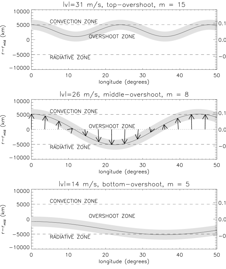
Figure 7: Geometry of a flux tube deformed by azimuthally periodic flows, at three initial locations (solid lines): (from top to bottom of the figure) the top, the middle, and the bottom of the overshoot region. The latitude is $30^{\circ}$ and the field strength is $6\times 10^{4}$ G. The distance from the middle of the overshoot region in kilometres is shown on the left axis, and in units of local pressure scale height (at $r=r_{\rm mid}$) on the right axis. The azimuthal wavenumber is chosen such that the troughs or crests of the tube partially enter the convection or the radiative zones. The radius of the tube is 1000 km. Arrows denote the relative strength of the resultant perturbation, which is led by the external flow.

We begin the analysis by finding the extreme values of the velocity amplitude, that displaces parts of the flux tube to the boundaries of the overshoot layer. Figure 7 shows the spherical perturbation $\xi_{r}$ as a function of $\phi$ at three depths in the overshoot region for a flux tube with $B_{0}=6\times 10^{4}$ G, $\lambda_{0}=30^{\circ}$, and $R_{t}=1000$ km. The velocity amplitudes corresponding to each of these three depths were adopted from the convection zone model of Skaley & Stix (1991). The azimuthal wavenumber were chosen such that in each case the crests or the troughs of the perturbed tube come very close to the boundaries of the overshoot layer. We call this azimuthal wavenumber $m_{\rm crit}$ and the resulting perturbation the critical perturbation. At the bottom of the overshoot region, the flow must be very extended ($m\lesssim 5$) to destabilise the flux tube. In higher layers of the overshoot region, narrower flows ($m\lesssim 8$ and $m\lesssim 15$) can have a destabilising effect. The critical azimuthal wavenumber required to carry the tube to the boundaries of the overshoot region, $m_{\rm crit}$, decreases with increasing depth. The relationship between $\xi_{r}$, $m$, and the radial location of the tube is determined by 1) magnetic curvature force, which increases with $m$, and 2) the convective velocity, which decreases with depth in the overshoot region.

3.1.2 Parameter study

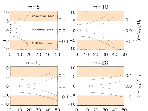
Figure 8: Variation in the maximal displacement of flux tubes by azimuthally periodic perpendicular flows with four different azimuthal wavenumbers, $m$, as a function of flow speed ($B_{0}=6\times 10^{4}$ G, $R_{t}=1000$ km). The vertical axes denote the radial distance with respect to the middle of the overshoot region (on the right axes in units of the local pressure scale height at the mid-overshoot region). Solid lines show the maximal downward displacement of the troughs of a tube starting in the bottom of the overshoot region. Dashed lines show the maximal displacement for the troughs and crests of tubes starting in the middle of the overshoot region, and the dash-dotted lines show the displacement of the crests of tubes starting near the top of the overshoot region. For clarity, the effect of upward (downward) flows on flux tubes near the bottom (top) of the overshoot region is not shown. The shaded regions denote the radiative zone below and the convection zone above.

The parameters describing the initial condition of the flux tube are the field strength, cross-sectional radius, initial radial position, and latitude. The parameters pertaining to the external flow are the azimuthal wavenumber and the velocity amplitude. In the following, we shall evaluate Eq. (7) and Eqs. (32)-(34) for given sets of parameters, in order to find the perturbation amplitude as functions of parameters related to the flow and the flux tube.

Dependence on the flow velocity and the azimuthal wavenumber.

Figure 8 shows the variation in $r-r_{\rm mid}$, which is the radial distance of the crest of the perturbed tube from the middle of the overshoot region, as a function of the velocity amplitude of the radial flow for various azimuthal wavenumbers. The minimum flow velocity required to advect the flux tube up to the convection zone or down to the radiative zone boundaries corresponds to the intersections of the curves with the boundaries of the overshoot layer. For a fixed flow speed and increasing $m$, it becomes more difficult to displace the tube crests from the equilibrium configuration, because the magnetic curvature force increases. For a given $m$, faster flows lead to larger perturbations. In the case for which the tube extends between the boundaries of the overshoot layer, the variation in buoyancy along the tube can be significant, because the superadiabaticity changes by about three orders of magnitude between the upper and lower boundaries (cf. Sect. 2.3, Fig. 4).

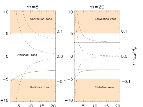
Figure 9: Displacement of flux tubes by radial external flows that are periodic in azimuth, as a function of field strength. The left panel is for $m=8$, and the right panel for $m=20$, to show the contrast between the effects of flows with large and small wavelengths. The radius, the latitude, the initial depth of the flux tubes, the vertical axes, and the line styles in the plots are the same as in Fig 8. The tube is subjected to an azimuthally periodic flow with an amplitude of 10, 26, 31 m s^-1 for the bottom, middle, and top of the overshoot region, respectively. The long dashed lines indicate the boundaries of the radiation and convection zones.

At the top of the overshoot region, a small-scale deformation (a high $m$) can drive the flux tube into the convection zone proper, whereas for the bottom of the overshoot region, coherent downflows on a rather large scale ($m\sim 5$) are required to push the tube down to the radiative zone. However, the true depth of penetration close to the radiative zone cannot be estimated in this way, because the superadiabaticity decreases strongly, and thus the linear approach becomes inapplicable. Indeed, the superadiabaticity becomes strongly negative so that the stable stratification largely inhibits any further downward penetration (see Sect. 2.4).

Dependence on the magnetic field strength.

Figure 9 shows the variation in the displacement amplitude as a function of its field strength, for $R_{\rm t}=10^{3}$ km, and the amplitude of the azimuthally periodic perpendicular flow is assumed to be $14$ m s^-1 at the bottom, $26$ m s^-1 at the middle, and $31$ m s^-1 at the top of the overshoot region, as in Fig. 7. As the azimuthal wavenumber of the flow is increased, the tension force resists the deformation of the tube more strongly, so that the perturbation weakens. For $B_{0}\gtrsim 10^{5}$ G and $m\gtrsim 10$, the deformation of the tube by the flow becomes smaller than $200$ km. For $m=20$, a perpendicular flow with a speed of $26$ m s^-1, applied to a tube with $B_{0}=10^{5}$ G, located at the middle of the overshoot region, displaces it by an extent of about $5\times 10^{-3}H_{p}$ ($\sim$300 km). The corresponding relative change in superadiabaticity between the depths of the crests and the troughs is $\Delta\delta\lesssim 10^{-7}$ (see Fig. 5), so the $\delta$-effect is ineffective in this case.

Dependence on the tube radius.

We now set the field strength to $B_{0}=6\times 10^{4}$ G and vary the tube radius, $R_{\rm t}$. The resulting functional dependence is shown in Fig. 10 for $m=8$ and $m=20$, for tubes starting at the three sets of depths and convective speeds chosen above for Fig. 9. Because the drag force is inversely proportional to $R_{t}$, thicker tubes are less affected by the flow. For $m=20$, tubes thicker than about 2000 km in diameter do not reach the boundaries of the overshoot region. At first glance, this indicates that thicker tubes may be stored in the overshoot region for longer times than thinner tubes. However, diameters larger than about a few thousand kilometres are not relevant to the present context, because the thin flux tube approximation is not valid if the tube diameter is comparable to the thickness of the overshoot layer: the radial variation in superadiabaticity across the tube becomes non-negligible, inducing a strong variation in the buoyancy over the tube cross-section (see Fig. 4).

The upper horizontal axis in Fig. 3 shows the perpendicular velocity amplitude of the external flow, leading to a given maximum radial displacement of the flux tube, $\Delta r=2|\xi_{r}|$, for $m=5$. Using the correspondence between $\varv_{\perp}$ and $|\xi_{r}|$ (Sect. 3.1.1), we can make the following estimation, using Fig. 3. A toroidal flux tube with $\lambda_{0}=30^{\circ}$, $B_{0}=7\times 10^{4}$ G, and $R_{\rm t}=10^{3}$ km can be stored in the middle of the overshoot region for about 3 years, provided that the external flow velocity does not exceed about $10\leavevmode\nobreak\ {\rm m\leavevmode\nobreak\ s}^{-1}$. This semi-analytical estimate concerning the storage of a magnetic flux tube in the overshoot layer is tested using nonlinear numerical simulations involving a localised downflow, in Sect. 3.2.2.

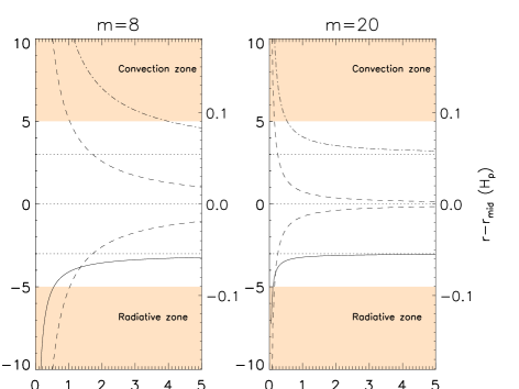
Figure 10: Same as Fig. 9, for $B_{0}=6\times 10^{4}$ G and varying tube radius.

3.2 Localised radial flow

We next consider the effects of both a localised radial flow, which has a finite extension in azimuth and latitude, and a longitudinal flow. The former describes, e.g., a convective downdraft penetrating into the overshoot layer, and the latter is required to define the initial mechanical equilibrium state.

3.2.1 Linear analysis

Before treating the nonlinear evolution of flux tubes under the combined effects of a localised downflow and the longitudinal flow, we develop an analytical approach to help us to understand the basic physics. We consider a toroidal flux tube subject to a localised downflow in the middle of the overshoot region, and describe the downward flow speed by a Gaussian function of the azimuth and obtain the stationary solution in a way similar to the one in Sect. 3.1. The description of the flow field and the stationary solution for the displacement are given in Appendix A.2. Figure 11 shows the radius-azimuth diagrams in which the dashed curves represent the stationary solutions for a flow with $\varv_{\rm max}=-10$ m s^-1 (minus sign means that the flow is directed downward) and various field strengths. For simplicity, the flux tube is located in the equatorial plane. For $B_{0}=10^{4}$ G, the downflow leads to a valley-shaped deformation in the flux tube. In this case, the shape of the flux tube is mostly determined by the azimuthal dependence of the perpendicular flow speed. For $B_{0}=3\times 10^{4}$ G and $B_{0}=4\times 10^{4}$ G, magnetic tension increasingly affects the stationary equilibrium shape of the flux tube. For a sufficiently strong magnetic field, a localised downflow leads to a deformation with a larger azimuthal extension than that of the downflow itself, owing to magnetic tension.

3.2.2 Nonlinear simulations

We assume a Gaussian profile for the external flow field,

$$\varv_{\perp}=a(t)\cdot\varv_{\max}\exp\left[\frac{-(r-r_{\rm m})^{2}}{2\sigma_{r}^{2}}-\frac{(\phi-\phi_{\rm m})^{2}}{2\sigma_{\phi}^{2}}-\frac{(\theta-\theta_{\rm m})^{2}}{2\sigma_{\theta}^{2}}\right],$$ (8)

where $a(t)$ describes the time variation. We set $r_{\rm m}=5.12\times 10^{10}$ cm and $\sigma_{r}=5000$ km, $\theta_{\rm m}=90^{\circ}$, $\phi_{\rm m}=180^{\circ}$, so that the flow speed has its maximum value, $\varv_{\rm max}$, at the upper boundary of the overshoot region, and falls to about one fifth of its maximum in the middle of the overshoot region. The lateral extensions $\sigma_{\phi}$ and $\sigma_{\theta}$ are free parameters. For all the simulations, the flux tube is located in the middle of the overshoot layer, and its cross-sectional radius is $10^{3}$ km.

Stationary flow (SF)

To test whether the stationary equilibria predicted in Sect. 3.2.1 can occur in the nonlinear case, we carried out numerical simulations by applying a localised downflow, which becomes stationary after a given time, $t_{s}=100$ days. We consider a toroidal flux tube, which is initially in mechanical equilibrium. We assume that an external downflow gradually develops around the point $(r_{\rm m},\theta_{\rm m},\phi_{\rm m})$, such that the time profile in Eq. (8) is assumed to be

$$a(t)=\left\{\begin{array}[]{r@{\quad:\quad}l}t/t_{s}&{\rm if}\leavevmode\nobreak\ t\leqslant t_{s}\\ 1&{\rm if}\leavevmode\nobreak\ t>t_{s}.\end{array}\right.$$ (11)

Figure 11: The radial position of an equatorial flux tube as a function of the azimuth, as determined by linear analysis (dashed curves, $\varv_{\rm max}=-10$ m s ^-1), and by nonlinear simulation of the SF50 case, after 8 months (solid curves). The internal flow (in the rest frame of the external medium) is from left to right. The initial field strength is different in each panel. The initial radial position is $r_{0}=5.07\times 10^{10}$ cm (the middle of the overshoot region). The dash-dotted horizontal lines indicate the boundaries of the overshoot region.

We present two subsets of simulations in this section: for the subset SF50, $\varv_{\rm max}=50$ m s^-1, and for SF10 $\varv_{\rm max}=$10 m s^-1. For each subset, the free parameters are the latitude, magnetic field strength, and the azimuthal and latitudinal extensions $(\sigma_{\phi},\sigma_{\theta})$ of the downflow, with the condition $\sigma_{\phi}=\sigma_{\theta}$. We define the “rise time” of an unstable flux tube as the time between $t=0$ and the end of the simulation when the tip of the rising loop arrives at about $r=0.98R_{\sun}$, where the thin flux tube approximation breaks down.

Snapshots from the set SF50 at $t=8$ months for various initial field strengths are shown with solid curves in Fig. 11, in comparison with the linear results for stationary equilibrium (Sect. 3.2.1). The direction of the internal flow along the flux tube is from left to right. The stationary solution is nearly identical to the nonlinear simulation snapshot for $B_{0}=10^{4}$ G. The broadening of the submerged part for higher $B_{0}$ (see Sect. 3.2.1) is visible in the numerical solutions. However, the simulations deviate from the linear results substantially on the left side of the downflow region, to an increasing extent for higher $B_{0}$. The azimuthally symmetric external downflow deforms the flux tube in an asymmetric form, owing to the internal flow. The central part of the tube reaches a dynamical equilibrium after about 100 days, whereas the tube as a whole never comes to equilibrium in any case: for low field strengths ($1-3\times 10^{4}$ G), the upward portion creates a transverse wave, which propagates leftward (retrograde). In the course of its subsequent evolution, the wave energy is transferred to lower azimuthal modes, while the submerged portion of the tube persists as long as the downflow speed is kept constant. For higher values of $B_{0}$, the magnetic tension force limits the extent of the downward displacement, whereas the excess magnetic buoyancy in the left wing is enhanced. This leads to a Parker-unstable loop for $B_{0}\gtrsim 5\times 10^{4}$ G, because the top of the loop reaches layers of sufficiently high superadiabaticity, and the density deficit in the loop top increases with time.

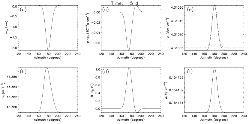
Figure 12: Physical quantities illustrating the effect of the external downflow, as a function of azimuth. The snapshots are taken at $t=5$ days of the SF50 simulation run for $B_{0}=5\times 10^{4}$ G. The external downflow is centred around $\phi=180^{\circ}$, which is indicated by a vertical line. We plot (a) the radial displacement of the tube from its initial position, (b) the internal flow speed, (c) the difference between the internal and external densities, (d) the deviation of field strength from $B_{0}$, (e) the internal pressure (dashed line shows the external pressure), and (f) the internal density.

To explain the physical reasons for the asymmetric deformation, we show in Fig. 12 the azimuthal profiles of various physical variables at an early stage of the simulation ($t=5$ days), for the SF50 case, where $B_{0}=5\times 10^{4}$ G. Once the external downflow begins to advect a part of the tube downward to a smaller radius (Fig. 12a), angular momentum conservation leads to a local increase in the internal flow speed (b). The maximum internal flow speed is reached at the left wing of the submerged portion of the tube, because of the additional acceleration by the component of gravity along the tube. Through the right side of the submerged part, the internal flow decelerates back to its initial equilibrium speed. This asymmetric flow leads to a density deficit at the left part and a density excess at the right side (c). The resulting positive buoyancy in the left part increases with time and forms an upward moving loop, which is driven further by the accelerating internal flow on the right wing of the loop and the higher superadiabaticity at the top location (see Fig. 11, the bottom panel). Starting from the initial phases, the accelerating flow also leads to a slightly lower internal pressure at the left part (e). To balance the external pressure, the magnetic field strength increases on the left part (d), and this contributes to the subsequent growth of the magnetic buoyancy instability. For $B_{0}\lesssim 5\times 10^{5}$ G, the instability does not set in, because the internal flow required for the initial mechanical equilibrium is too slow for a sufficient density deficit to develop on the left wing of the submerged part. For $B\lesssim 4\times 10^{4}$ G, the transversal wave propagates leftward and quits the downflow region, well before a sufficient density deficit on the left wing develops.

Table 2 presents the rise times (in cases of instability) of flux tubes at different latitudes, field strengths, and lateral extensions of the downflow, for SF50 and SF10 cases. Linearly Parker-unstable cases are shown in italics.

Table 2: Rise times for stationary flow simulations.

		$\varv_{\rm max}$ = -50 m s-1
			$\tau_{\rm rise}$ (days)
$\lambda_{0}$ (deg)	$B_{0}$ ($10^{4}$ G)	$\sigma_{\phi,\theta}=2^{\circ}$	$\sigma_{\phi,\theta}=5^{\circ}$	$\sigma_{\phi,\theta}=10^{\circ}$
0	1	stable	stable	stable
0	3	stable	stable	stable
0	5	723	492	397
0	6	920	324	259
0	7	445	269	207
0	10	662	700	191
10	5	661	464	369
10	7	439	265	204
30	7	1791	268	192
40	4	stable	2516	1364
		$\varv_{\rm max}$ = -10 m s-1
			$\tau_{\rm rise}$ (days)
$\lambda_{0}$ (deg)	$B_{0}$ (T)	$\sigma_{r,\theta}=2^{\circ}$	$\sigma_{r,\theta}=5^{\circ}$	$\sigma_{r,\theta}=10^{\circ}$
0	5	stable	stable	stable
0	7	stable	stable	stable
0	10	659 (m=1)	608	567
0	12	147 (m=2)	140	136
10	7	stable	stable	stable
30	7	stable	stable	4167

For the set SF50, the cases with field strengths up to $5\times\leavevmode\nobreak\ 10^{4}$ G are stable. For the linearly Parker-stable cases ($B<9\times 10^{4}$ G), greater lateral extensions of the downflow would destabilise the tube, because for larger $\sigma_{\phi}$, the magnetic curvature force is smaller, thus the perturbed part of the tube can descend deeper, increasing further the internal flow speed in the left wing. In this regime, a stronger magnetic field also leads to faster growth of the loop, because the internal equilibrium flow becomes faster, which develops the density deficit on the left wing more rapidly. For the linearly Parker-unstable cases (denoted in italics in Table 2), the rise times are generally longer, because in most cases the initial central deformation of the tube excites standing waves with $m=5$. This limits the growth of the loop on the left side of the submerged part, and the flux tube enters the convection zone only after the growth of an oscillatory instability with $m=1$. For SF10 simulations, the downflow is too weak to trigger nonlinear buoyancy instability, so the linearly Parker-stable cases are stable in the nonlinear case, whereas for $B_{0}\gtrsim 10^{5}$ G Parker instability sets in, in accordance with the prediction of linear perturbation theory.

Transient flow (TF)

Downflows penetrating into the solar overshoot layer are probably transient, i.e., they are decelerated by the increasingly stable stratification on their way towards the radiative zone. To test the consequences of such a flow, we assume a Gaussian profile for the time variation in the downflow speed in Eq. (8), such that

$$a(t) = \exp\left[\frac{-(t-t_{\rm m})^{2}}{2\sigma_{t}^{2}}\right],$$ (12)

where $t_{\rm m}$ is the time when the maximum flow speed is reached. The flow sets in at $t=0$ with $\varv=10^{-3}\varv_{\rm max}$. The initial effect of the downflow on the flux tube is similar to that in the SF case. However, once the downflow ceases, it leaves behind transversal tube waves propagating along the tube, which interfere with each other. For unstable cases, the relative longitudinal flow leads to instability by frictional coupling, with the growth rate depending on the internal flow velocity (thus the field strength) and the perturbation amplitude (cf. Sect. 2). The difference between SF and TF is that in the former case the stationary flow had continued for a sufficiently long time to allow the formation of a buoyant loop on one side of the downflow region (Fig. 12).

We carried out a systematic survey of numerical simulations by varying the flow duration, $2t_{\rm m}$, and velocity amplitude, $\varv_{\rm max}$ in the ranges $0<|\varv_{\rm max}|<50$ m s^-1 and $0<2t_{\rm m}<200$ d, for $\lambda_{0}=10^{\circ}$. The constants $t_{\rm m}$ and $\sigma_{t}$ were chosen such that the initial speed is of the order of $10^{-3}\varv_{\rm max}$. For $B_{0}\lesssim 5\times 10^{4}$ G, the growth time of the friction-induced instability is longer than the upper time limit, which we set to be 7 years. Instabilities with growth times longer than a few years are not relevant in the present context, because within that time the toroidal magnetic field must be amplified in the solar tachocline to its full strength. For $B_{0}=7\times 10^{4}$ G, which is about 20 kG lower than the Parker instability threshold for linear perturbations, the flux tube develops an unstable loop within about 4 years for some values of $(|\varv_{\rm max}|,2t_{\rm m})$.

The evolution of the tube for $|\varv_{\rm max}|=20$ m s^-1 and downflow durations of 60 days (TF60) and 180 days (TF180) is shown in supplementary animations (see the online appendix, Figs. 15 and 16). The tube rises over about 10 years for TF60, and about 3.3 years for TF180. In the initial stages of TF180, the evolution of the tube resembles the strong-field behaviour for the SF50 case (cf. Fig. 11, bottom panel).

Figure 13 shows the rise times as a function of $|\varv_{\rm max}|$ and $2t_{\rm m}$. Only the final month of the rise time is spent in the convection zone proper, the rest being spent in the overshoot region. A relatively fast downflow ($|\varv_{\rm max}|\lesssim$ 40 m s^-1) lasting less than about 2 months, or a slow downflow ($|\varv_{\rm max}|\lesssim$ 20 m s^-1) lasting less than about 6 months allow the storage of the flux tube in the overshoot region for more than about 3 years. As a rough estimate of the flow duration in the overshoot region, we also calculated the convective turnover time, $H_{p}/\varv_{\rm max}$, in the middle of the overshoot layer. To lead to the formation of an unstable flux loop out of a tube with $B_{0}=7\times 10^{4}$ G, either the flow should last much longer than the turnover time or the flow should reach much higher speeds than the range assumed here.

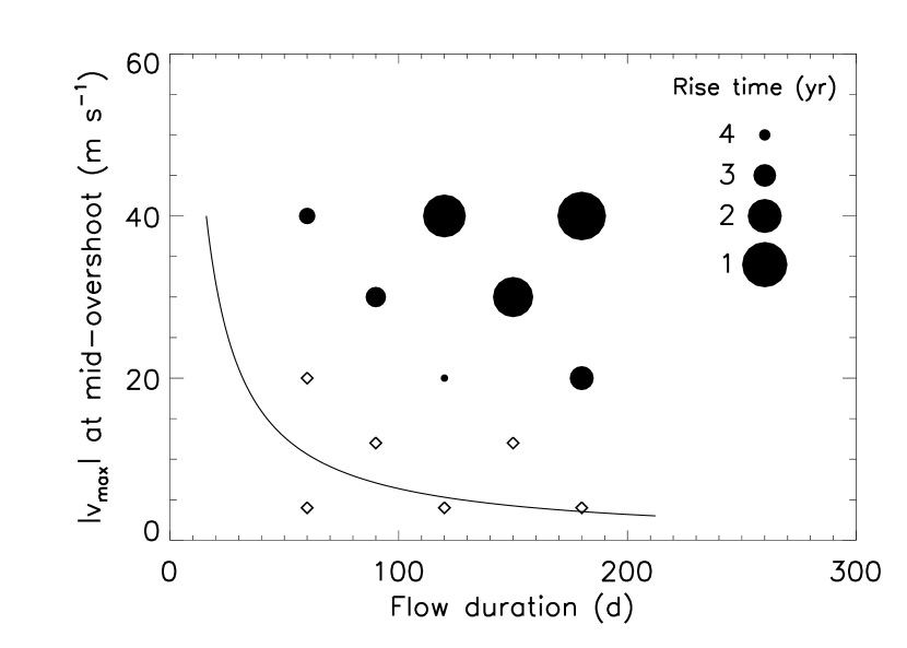
Figure 13: The variation in the rise time for a linearly Parker-stable flux tube in the mid-overshoot region, as a function of the duration and maximum speed of the localised external downflow with $\sigma_{\phi,\theta}=5^{\circ}$, $\theta_{\rm m}=180^{\circ}$, $r_{\rm m}=512$ Mm (convection zone – overshoot layer boundary) for the TF simulations. The field strength and latitude of the initial tube are $B_{0}=7\times 10^{4}$ G and $\lambda_{0}=10^{\circ}$ (cf. Fig. 1). The diamonds represent the “stable” cases, for which no emergence takes place before 7 years, and the size of the filled circles is inversely scaled with the rise time. The solid curve shows the convective turnover time as an indicator for the flow duration, estimated as $H_{p}/\varv_{\rm max}$.

4 Discussion

We have investigated flow-induced instabilities of toroidal magnetic flux tubes in the solar overshoot region, to extend the results of paper III to the nonlinear regime and to quantitatively estimate the effects of convective flows on the storage of magnetic flux in the solar overshoot region. Our simulations confirm the main results of the linear stability analysis of paper III (Sect. 2.2). The perpendicular velocity component can be approximated generally in the form $\varv_{\perp}\sim|\xi_{r}|\leavevmode\nobreak\ \leavevmode\nobreak\ \Re{\rm e}(\omega_{\rm f})$, where $|\xi_{r}|$ is the amplitude of the radial perturbation and $\omega_{\rm f}$ is the eigenfrequency of the fastest growing unstable wave mode. Substituting this expression into Eq. (3), we obtain

$$\alpha\sim\frac{C_{\rm D}\varv_{\perp}}{\pi R_{\rm t}}\leavevmode\nobreak\ \leavevmode\nobreak\ \propto\leavevmode\nobreak\ \leavevmode\nobreak\ |\xi_{r}|\leavevmode\nobreak\ \leavevmode\nobreak\ \Re{\rm e}(\omega_{\rm f}),$$ (13)

For a given value of $\Re{\rm e}(\omega_{\rm f})$, which is specified for a given set of $\delta$ (depth), $\lambda_{0}$, and $B_{0}$, $\alpha$ increases with increasing perturbation amplitude, as shown by numerical simulations in Sect. 2.2 (Fig. 2). Considering the relations obtained in Sect. 3.1, a perpendicular flow with $\varv_{\perp}\simeq 1\leavevmode\nobreak\ {\rm m\leavevmode\nobreak\ s}^{-1}$ and $m=5$ in the middle of the overshoot region can displace a flux tube with $B=7\times 10^{4}$ G to $|\xi_{r}|\simeq 2500$ km (cross symbols in Fig. 2). Substituting $\varv_{\perp}$ into Eq. (13), this amounts to $\alpha\simeq 3\times 10^{-7}$, which is of the same order as the value chosen for the full curve in Fig. 2. Considering the numerical results in Sect. 2.2 (see Fig. 3), we conclude that an external flow with a velocity amplitude of 1-10 m s^-1 perpendicular to the tube axis leads to instability with a growth time of the order of 1000 days ($\sim$2.74 years) or longer. This range of velocities is consistent with the estimates of van Ballegooijen (1982) for the convective velocities in the overshoot region, supporting the possibility of storing magnetic flux tubes that contain fluxes of the order of $10^{21}$ Mx. In a more recent study, Brummell et al. (2002) carried out 3D numerical simulations of penetrative convection, which infer penetration depths between $0.02H_{p}$ and $0.11H_{p}$, when they extrapolate the dimensionless numbers in their simulations to solar values. These values are also comparable to the radial perturbation amplitudes that we have assumed here.

The numerical experiments presented in Sect. 2.3 have shown us that the nonlinear instability occurring in the linearly Parker-stable regime is induced mainly by the frictional coupling of the flux tube with its surroundings. We have also found unstable flux tube configurations, for which the $\delta$-effect plays a significant role in the dynamics. These numerical experiments were made without considering the drag force and in the bottom of the overshoot layer, where the radial gradient of superadiabaticity is steeper than in the remainder of the overshoot region. This result may be relevant during the final phases of the decay of the large-scale toroidal field in the Sun: if we assume that the toroidal flux at the upper layers of the overshoot region has already been removed to a large extent at this phase, a flux tube that forms near the bottom of the overshoot region can be destabilised rapidly by strong (possibly rare) convective downflows, leading to a few active regions during a solar minimum. We conjecture that the $\delta$-effect is not the main source of flux loss from the overshoot layer, with a possible exception in the bottom of the overshoot region, provided that overshooting convective flows are sufficiently strong.

In test simulations, we have found that for perturbations larger than about $10^{-3}H_{p}$ ($\sim$55 km), the growth rates start to deviate from the predictions of linear stability analysis (Ferriz-Mas & Schüssler 1995), because nonlinear effects govern the dynamics and determine the growth rate of instability, through either the friction-induced instability (Sect. 2.2) or the $\delta$-effect (Sect. 2.3), depending on the depth and the longitudinal flow speed.

In seeking possibilities of a slingshot effect that leads to small-scale loops in thin flux tubes, we have found that this effect is inefficient in removing magnetic flux from the overshoot region. The common result of the simulations is that a loop driven by a transient downflow hits the radiative zone and bounces back rapidly. However, in its way through the overshoot region it is strongly decelerated mainly by friction.

In a parameter study surveying analytical estimates of the displacement amplitude as a function of field strength (Sect. 3.1.2), we have found that a flow pattern with $m=20$ and $\varv_{\perp}=26$ m s^-1 acting on a tube with $B_{0}=10^{5}$ G leads to a perturbation of about 300 km. The corresponding difference in the superadiabaticity of the stratification is $\Delta\delta\simeq 10^{-7}$ (see Fig. 5). Therefore, we do not expect azimuthally periodic flows with short wavelengths ($m\gtrsim 20$) to trigger flux tube instabilities for $B_{0}\lesssim 10^{5}$ G, provided that the displacement is less than about 300 km, in other words, $\varv_{\perp}\lesssim 26$ m s^-1.

After understanding the fundamental effects of azimuthally periodic flows on flux tubes, we have considered the case of a localised downflow in Sect. 3.2. For a given flow pattern, we have calculated the evolved states of flux tubes with various field strengths corresponding to linearly Parker-stable cases, using the steady-state approximation in conjunction with numerical simulations. The experiments presented in Fig. 11 can also be interpreted in terms of a toroidal field strength increase with time, in the rising phase of solar activity. As the toroidal field is amplified, localised downflows will have stronger disruptive effects on flux tubes, owing to the increasing internal flow speed, which is determined by the mechanical equilibrium condition. For a stationary downflow, we thus suggest that the lower limit to the field strength for which flux loops start entering the convection zone is of the order of $5\times 10^{4}$ G for the middle of the overshoot region.

Proceeding to non-stationary, transient flows, we have set up a survey of simulations for $B_{0}=7\times 10^{4}$ G in the middle of the overshoot region for Gaussian time profiles (TF case). Depending on the dynamical properties of the downflow, we have calculated the evolution of a flux tube with an upper time limit of 7 years. However, in the first 7 years of an activity cycle, the amplification of the large-scale toroidal field in the tachocline cannot be neglected. If a flux tube with a sub-critical field strength, say $B_{0}=7\times 10^{4}$ G, remains in the overshoot region for a few years, it is likely that it will be amplified and eventually form a Parker-unstable loop for $B_{0}\sim 10^{5}$ G, which can lead to the formation of active regions with the observed properties in the photosphere.

We have found that the storage of a toroidal magnetic flux tube with $\Phi\simeq 2\times 10^{21}$ Mx for times comparable to the dynamo amplification time is possible. Within the scope of the thin flux tube approximation and non-local mixing length models of the solar interior, we have not found any significant (hydrodynamically or magnetically induced) stability problem that impedes the construction of Parker-unstable tubes with fluxes of the order of $10^{22}$ Mx.

We have considered the problem of storing a toroidal flux tube field rather than the problem of building up the magnetic field in the first place. We have assumed that the field is amplified in the overshoot region, e.g., by rotational shear, on a timescale of a few years. The stationary equilibria of subcritical flux tubes ($B_{0}\lesssim 10^{5}$ G) advected by radial flows indicate deformations comparable to the size of the overshoot region (see Fig. 9). On the one hand, it may be argued that these deformations can destabilise the tube, e.g., by $\delta$-effect, at times comparable to the duration of overshooting convective flows (see Sect. 3.1). However, nonlinear simulations (Fig. 11) show deviations from linear estimates, as the field strength increases towards $5\times 10^{4}$ G: the tube is destabilised as the field strength is increased. These simulations indicate that toroidal magnetic fields can be stored within the overshoot region in the course of their amplification up to the critical field strength ($10^{5}$ G) required to explain general properties of active regions. Our results can be cross-checked when the spatio-temporal structure of penetrative convection near the bottom of the convection zone is observed by helioseismology, or when 3D hydrodynamic simulations with realistic Reynolds numbers and sufficiently high resolution become available.

5 Conclusions

Based on analytical steady-state approximations and nonlinear simulations of toroidal flux tubes in the solar convective overshoot region, we reach the following conclusions:

• The flow instability driven by the frictional coupling of transversal MHD waves with external flows is nonlinear in the sense that the growth rate is a function of the initial perturbation amplitude. This is consistent with the results of the linear stability analysis of paper III, in which the parameter $\alpha$ is proportional to the speed of the perpendicular flow and thus to the amplitude of the subsequent perturbation. Therefore, the perturbation amplitude determines the $\alpha$ parameter in the linear analysis.

• Significant buoyancy variations ($\delta$-effect) along magnetic flux tubes can lead to a nonlinear buoyancy instability. The $\delta$-effect most likely occurs in regions of large radial gradients of superadiabaticity such as the bottom of the overshoot layer, where a sufficient $\delta$ variation along the tube ($\Delta\delta\gtrsim 10^{-6}$) is easier to attain than in the upper layers.

• For flux tubes in the solar overshoot layer, we have established links between the perpendicular flow velocity amplitude, its spatial (azimuthal) extension, and the resulting radial displacement and instabilities induced by $\delta$-effect or longitudinal flows.

• To store magnetic flux with flux densities between $10^{4}$-$10^{5}$ G for times comparable to the dynamo amplification time in the convective overshoot layer, the average flow speed and the flow duration must not exceed about 50 m s ^-1 and 100 days, respectively, and that the azimuthal extension of the flow is lower than about $10^{\circ}$. If we assume that these conditions prevail in the solar overshoot region, then magnetic fluxes of up to $10^{22}$ Mx can be stored within thin flux tubes during the dynamo amplification phase.

Appendix A Flux tube subject to radial flows

The equations for a flux ring at an arbitrary latitude $\lambda_{0}$, in the limit of $\beta\gg 1$, are given by Ferriz-Mas & Schüssler 1995 (Sect. 4.1). Consider that a flow along the spherical radial direction with an amplitude $\varv_{\perp}$, is applied to a flux tube with radius $R_{\rm t}$ located at latitude $\lambda_{0}$. This flow will exert a drag force perpendicular to the tube axis, $F_{\mathrm{D}}=\rho_{e0}\varv_{\perp}^{2}/\pi R_{\mathrm{t}}$, where $\rho_{e0}$ is the unperturbed external density. After a certain time, the drag force and the restoring forces of magnetic tension, Coriolis, and buoyancy will balance each other and a stationary equilibrium will be reached. Adopting the equation of motion for linearised perturbations (Ferriz-Mas & Schüssler 1995) for the stationary force equilibrium yields the inhomogeneous system of equations

$$2f^{2}\frac{\partial^{2}\xi_{R}}{\partial\phi^{2}}+C_{\phi}\frac{\partial\xi_{\phi}}{\partial\phi}+C_{R}\xi_{R}+C_{z}\xi_{z} = \frac{\tau^{2}}{\rho_{e0}}F_{\rm D}(\phi)\cos\lambda_{0},$$ (14)

$$2f^{2}\frac{c_{T}^{2}}{\varv_{A}^{2}}\frac{\partial^{2}\xi_{\phi}}{\partial\phi^{2}}+A_{R}\frac{\partial\xi_{R}}{\partial\phi}+A_{z}\frac{\partial\xi_{z}}{\partial\xi_{\phi}} = 0,$$ (15)

$$2f^{2}\frac{\partial^{2}\xi_{z}}{\partial\phi^{2}}+D_{\phi}\frac{\partial\xi_{\phi}}{\partial\phi}+D_{R}\xi_{R}+D_{z}\xi_{z} = \frac{\tau^{2}}{\rho_{e0}}F_{\rm D}(\phi)\sin\lambda_{0},$$ (16)

where

$$A_{R}=4f\left(f-\frac{\cos\lambda_{0}}{2\gamma}\right),A_{z}=-\frac{2f}{\gamma}\sin\lambda_{0},$$

$$C_{\phi}=-A_{R},\leavevmode\nobreak\ \leavevmode\nobreak\ \leavevmode\nobreak\ C_{R}=\frac{4f}{\gamma}\cos\lambda_{0}+\Delta\cos^{2}\lambda_{0},$$

$$C_{z}=\left(\frac{2f}{\gamma}+\Delta\cos\lambda_{0}\right)\sin\lambda_{0},$$ (17)

$$D_{\phi}=-A_{z},\leavevmode\nobreak\ \leavevmode\nobreak\ \leavevmode\nobreak\ D_{R}=C_{z},\leavevmode\nobreak\ \leavevmode\nobreak\ \leavevmode\nobreak\ D_{z}=\Delta\sin^{2}\lambda_{0},$$

$$\Delta=\beta\delta-\frac{2}{\gamma}\left(\frac{1}{\gamma}-\frac{1}{2}\right).$$

Here we have assumed that the magnitude of the drag force is comparable to a first-order perturbation.

A.1 Azimuthally periodic flow

We define the flow velocity in the form $\varv_{\perp}=\cos(m\phi)$ for a given azimuthal wavenumber $m$. The resulting drag force is given by

$$F_{\rm D}(\phi,m) = \frac{\rho_{e0}\varv_{\perp 0}^{2}}{\pi R_{t}}\exp(im\phi),$$ (19)

where $\varv_{\perp 0}$ is the maximum value of the velocity. The resulting displacement is of the form

$$\xiup=\widehat{\xi_{m}}\exp(im\phi).$$ (20)

Substituting Eqs. (19 & 20) into Eqs. (14)-(16), we obtain

$$A\leavevmode\nobreak\ \leavevmode\nobreak\ \leavevmode\nobreak\ \leavevmode\nobreak\ \leavevmode\nobreak\ \leavevmode\nobreak\ \leavevmode\nobreak\ \leavevmode\nobreak\ \leavevmode\nobreak\ \leavevmode\nobreak\ \leavevmode\nobreak\ \leavevmode\nobreak\ \leavevmode\nobreak\ \leavevmode\nobreak\ \leavevmode\nobreak\ \leavevmode\nobreak\ \leavevmode\nobreak\ \leavevmode\nobreak\ \leavevmode\nobreak\ \leavevmode\nobreak\ \leavevmode\nobreak\ \leavevmode\nobreak\ \leavevmode\nobreak\ \leavevmode\nobreak\ \leavevmode\nobreak\ \leavevmode\nobreak\ \leavevmode\nobreak\ \leavevmode\nobreak\ \leavevmode\nobreak\ \leavevmode\nobreak\ \leavevmode\nobreak\ \leavevmode\nobreak\ \leavevmode\nobreak\ \leavevmode\nobreak\ \leavevmode\nobreak\ \leavevmode\nobreak\ \leavevmode\nobreak\ \leavevmode\nobreak\ \leavevmode\nobreak\ \leavevmode\nobreak\ \leavevmode\nobreak\ \leavevmode\nobreak\$$

$$\overbrace{\left(\begin{array}[]{ccc}C_{R}-2f^{2}m^{2}&imC_{\phi}&C_{z}\\ imA_{R}&-2f^{2}m^{2}c_{T}^{2}/\varv_{A}^{2}&imA_{z}\\ D_{R}&imD_{\phi}&D_{z}-2f^{2}m^{2}\end{array}\right)}\left(\begin{array}[]{c}\hat{\xi}_{R}\\ \hat{\xi}_{\phi}\\ \hat{\xi}_{z}\end{array}\right) =$$ (27)

$$\left(\begin{array}[]{c}-\frac{\tau^{2}}{\pi R_{\rm t}}\cos\lambda_{0}\varv_{\perp 0}^{2}\\ 0\\ -\frac{\tau^{2}}{\pi R_{\rm t}}\sin\lambda_{0}\varv_{\perp 0}^{2}\end{array}\right).$$ (31)

This equation can be solved in a straightforward way using Cramer’s rule. The solution for the complex amplitudes yields

$$\hat{\xi}_{R,m} = \frac{\tau^{2}m^{2}}{{\rm det}A}\frac{\varv_{\perp 0}^{2}}{\pi R_{\rm t}}\Bigg{\{}\cos\lambda_{0}\left[2f^{2}\frac{c_{\rm T}^{2}}{\varv_{\rm A}^{2}}(D_{z}-2f^{2}m^{2})-A_{z}D_{\phi}\right]$$ (32)

$$\hskip 44.0pt+\sin\lambda_{0}\left[A_{z}C_{\phi}-2f^{2}\frac{c_{\rm T}^{2}}{\varv_{\rm A}^{2}}C_{z}\right]\Bigg{\}},$$

$$\hat{\xi}_{\phi,m} = im\frac{\tau^{2}}{{\rm det}A}\frac{\varv_{\perp 0}^{2}}{\pi R_{\rm t}}\Bigg{\{}\cos\lambda_{0}\left[A_{R}(D_{z}-2f^{2}m^{2})-A_{z}D_{R}\right]$$ (33)

$$\hskip 44.0pt+\sin\lambda_{0}\left[A_{z}(C_{R}-2f^{2}m^{2})-A_{R}C_{z}\right]\Bigg{\}},$$

$$\hat{\xi}_{z,m} = \frac{\tau^{2}m^{2}}{{\rm det}A}\frac{\varv_{\perp 0}^{2}}{\pi R_{\rm t}}\Bigg{\{}\cos\lambda_{0}\left[A_{R}D_{\phi}-2f^{2}\frac{c_{\rm T}^{2}}{\varv_{\rm A}^{2}}D_{R}\right]$$ (34)

$$\hskip 35.0pt+\sin\lambda_{0}\left[2f^{2}\frac{c_{\rm T}^{2}}{\varv_{\rm A}^{2}}(C_{R}-2f^{2}m^{2})-A_{R}C_{\phi}\right]\Bigg{\}}.$$

Substituting each component (32)-(34) into Eq. (20), we obtain

$$\xi_{R}=\Re{\rm e}(\hat{\xi}_{R,m})\cos(m\phi),$$

$$\xi_{\phi}=-\Im{\rm m}(\hat{\xi}_{\phi,m})\sin(m\phi),$$

$$\xi_{z}=\Re{\rm e}(\hat{\xi}_{z,m})\cos(m\phi),$$

(35)

A.2 Localised flow

In the case of a localised perpendicular flow, we define the velocity and the drag force in the following forms:

$$\varv_{\perp}(\phi) = \exp\left(\frac{-\sin^{2}\phi/2}{\sigma^{2}}\right),$$ (36)

$$F_{\rm D}(\phi) = \frac{\rho_{e0}\varv_{\perp 0}^{2}}{\pi R_{t}}\sum_{m}\hat{g}_{m}\exp(im\phi),$$ (37)

where $g_{m}=\sum_{m}\hat{g}_{m}\exp(im\phi)$ is the Fourier transform of the function $\varv_{\perp}^{2}(\phi)$. For the resulting displacement, $\zetaup$, we follow the method described in Sect. A.1 and write the components in the Fourier series representation

$$\zeta_{R}=\sum_{m}\hat{\xi}_{R,m}\hat{g}_{m}\exp(im\phi),$$

$$\zeta_{\phi}=\sum_{m}\hat{\xi}_{\phi,m}\hat{g}_{m}\exp(im\phi),$$

$$\zeta_{z}=\sum_{m}\hat{\xi}_{z,m}\hat{g}_{m}\exp(im\phi),$$

(38)

where the complex constants $\hat{\xi}_{[R,\phi,z],m}$ are given by Eqs. (32)-(34). The final solution for the components of the perturbation resulting from a localised perpendicular flow has the form

$$\zeta_{R}=\sum_{m}\Re{\rm e}(\hat{\xi}_{R,m})\left[\Re{\rm e}(\hat{g}_{m})\cos(m\phi)-\Im{\rm m}(\hat{g}_{m})\sin(m\phi)\right],$$

$$\zeta_{\phi}=-\sum_{m}\Im{\rm m}(\hat{\xi}_{\phi,m})\left[\Im{\rm m}(\hat{g}_{m})\cos(m\phi)+\Re{\rm e}(\hat{g}_{m})\sin(m\phi)\right],$$

$$\zeta_{z}=\sum_{m}\Re{\rm e}(\hat{\xi}_{z,m})\left[\Re{\rm e}(\hat{g}_{m})\cos(m\phi)-\Im{\rm m}(\hat{g}_{m})\sin(m\phi)\right].$$

(39)

Appendix B The stationary equilibrium approximation

B.1 Comparison of azimuthal and radial effects

Suppose that a toroidal flux tube is in mechanical equilibrium. Then apply a localised external flow in the spherical radial direction. The parts of the tube affected by the flow are advected in the direction of the flow, until the drag force is balanced by the restoring forces of buoyancy and magnetic tension. To justify ignoring any displacement of mass elements along the tube, a necessary condition is that the time for the radial displacement, $\tau_{r}$, is short compared to that of the displacement along the tube axis (tangential perturbation, $\tau_{\phi}$ ), so that

$$\tau_{\phi}\equiv\frac{\pi r_{0}}{m|\dot{\xi}_{\phi}|}\gg\left|\frac{\xi_{R}}{\varv_{R}}\right|\equiv\tau_{R},$$ (40)

where $r_{0}$ is the radial coordinate of the equilibrium tube, $\dot{\xi}_{\phi}$ is the propagation velocity of the perturbation along the tube, and $\varv_{R}$ is the maximum flow speed, and $\dot{\xi}_{\phi}$ can be determined from the solution of the eigenvector problem using the linearised equation of motion for first-order perturbations (see Sect. B.2). The left-hand side of Eq. (40) represents a timescale for the re-establishment of hydrostatic equilibrium, and the right-hand side represents the time it takes for a dynamical balance between the drag force and the restoring forces is reached.

As an example, we consider an equatorial flux tube, in the middle of the overshoot layer. The external flow is assumed to be localised (Eq. 37) and downwards with a maximum speed of $10$ m s^-1. This is the same flow configuration as that described in Sects. 3.2.1 and A.2. For simplicity, we disregard the effects of longitudinal wave modes and the presence of azimuthal flow, which is required by the mechanical equilibrium condition. Table 3 shows the values for both sides of the inequality (40), as a function of the azimuthal wavenumber of the external flow, for $B_{0}=6\times 10^{4}$ G. We also give the values of the downward displacement amplitude, $\xi_{R}$, produced by the external downflow. For comparison, numerical simulations were performed by setting up azimuthally periodic flow configurations for various azimuthal wavenumbers. In each case, the flow sets in at $t=0$ and reaches its full strength ($|\varv_{\rm max}|=10$ m s^-1) in 30 days. The tabulated values are the maximum displacement at $t=240$ days, for which the drag force exerted by the external flow is already balanced by buoyancy and magnetic tension. The variation in displacement amplitude as a function of $m$ for azimuthally periodic flows shows general agreement with that for the linearly estimated amplitudes of each azimuthal wave mode corresponding to a localised downflow.

The ratio $\tau_{\phi}/\tau_{R}$ decreases for smaller $m$. When $\tau_{\phi}$ becomes comparable to $\tau_{R}$ (as the ratio falls below about 10), the azimuthal perturbation might have a significant effect on the density distribution along the tube, such that our assumption of a stationary equilibrium between the normal forces becomes inaccurate.

Table 3: Characteristic times for radial and azimuthal displacements.

$m$	$\xi_{R}$ (linear)	$\xi_{R}$ (num.sim.)	$\tau_{R}$ (d)	$\tau_{\phi}$ (d)	$\tau_{\phi}/\tau_{R}$ (d)
	(km)	(km)
3	14077	12180	16.3	85	5.2
4	4347	4037	5.0	202	40
5	2302	2366	2.7	290	109
6	1461	1531	1.7	358	211
7	1021	1044	1.2	408	345
8	757	731	0.9	445	509

B.2 Flux tube in the equatorial plane: eigenvector problem

For simplicity, we consider a flux tube in the equatorial plane, to obtain eigenvectors for the wave-like solutions of the perturbed flux tube. In this case, the momentum equation for linear perturbations is simpler than for a non-equatorial flux tube, and therefore it is simpler to make a physical interpretation.

To obtain relations between the flow velocity and the resulting displacement, we consider the linearised equations of motion for perturbations $(\xi_{R},\xi_{\phi},\xi_{\lambda})$, where $R$ is the distance from the rotation axis, $\phi$ is the longitude, and $\lambda$ is the latitude. Here, only radial and azimuthal components (perturbations in the $(R,\phi)$ plane) are considered, because the equation for the latitudinal component is decoupled in the equatorial plane. Following Ferriz Mas & Schüssler (1993), the linearised equations of motion for the perturbations in the $(R,\phi)$ plane read

$$\tau^{2}\left(\ddot{\xi}_{R}-2\Omega\dot{\xi}_{\phi}\right) = 2f^{2}\frac{\partial^{2}\xi_{R}}{\partial\phi_{0}^{2}}-4f\left(f-\frac{1}{2\gamma}\right)\frac{\partial\xi_{\phi}}{\partial\phi_{0}}+T\xi_{R},$$ (41)

$$\tau^{2}\left(\ddot{\xi}_{\phi}+2\Omega\dot{\xi}_{R}\right) = 2f^{2}\frac{\partial^{2}\xi_{\phi}}{\partial\phi_{0}^{2}}+4f\left(f-\frac{1}{2\gamma}\right)\frac{\partial\xi_{R}}{\partial\phi_{0}},$$ (42)

where

$$T = 2(\sigma-1)f^{2}+\frac{4}{\gamma}f-\frac{2}{\gamma}\left(\frac{1}{\gamma}-\frac{1}{2}\right)$$ (43)

$$+\beta\delta+\tau^{2}(\sigma-1)(\Omega_{\mathrm{e0}}^{2}-\Omega^{2}),$$

$$\tau \equiv \left(\frac{\beta H_{p}}{g_{0}}\right)^{1/2}=\sqrt{2}\frac{H_{p}}{\varv_{A}},$$ (44)

$$f \equiv \frac{H_{p}}{R_{0}}=\frac{p_{i0}}{g_{0}\rho_{i0}R_{0}},$$ (45)

$$\beta \equiv \frac{8\pi p_{i0}}{B_{0}^{2}}.$$ (46)

The meanings of the various symbols in the above equations are as follows: $H_{p}$ is the local pressure scale height, $\delta$ is the superadiabaticity, $p_{i0}$ and $\rho_{i0}$ are the equilibrium values for the pressure and density inside the tube, respectively, $r_{0}$ is the spherical radial position of the equilibrium tube, $\Omega$ and $\Omega_{e0}$ are, respectively, the angular velocities of the plasma in the tube and the external medium, $\varv_{A}$ is the Alfvén velocity, $B_{0}$ is the magnetic field strength, and $g_{0}$ the gravitational acceleration with a radial dependence $g\propto r^{\hskip 2.13394pt\sigma}$, where $\sigma$ is taken to be $-2$, which means that the small contribution of the mass inside the convection zone is neglected. The substitution of the ansatz

$${\bf\xi}_{m} = \widehat{\xi}_{m}\exp(i\omega t+im\phi).$$ (47)

into Eqs. (41)-(42) leads to the system of equations

$$(2f^{2}m^{2}-T-\tilde{\omega}^{2})\hat{\xi}_{R}+i\left[4fm\left(f-\frac{1}{2\gamma}\right)-2\tilde{\Omega}\tilde{\omega}\right]\hat{\xi}_{\phi}=0$$ (48)

$$-i\left[4fm\left(f-\frac{1}{2\gamma}\right)-2\tilde{\Omega}\tilde{\omega}\right]\hat{\xi}_{R}+(2f^{2}m^{2}-\tilde{\omega}^{2})\hat{\xi}_{\phi}=0.$$ (49)

For the existence of non-trivial solutions, the characteristic determinant must vanish. This yields the dispersion relation, which is a 4th-order polynomial in terms of the eigenfrequency. The eigenvector in the azimuthal direction is determined by one of the equations in the system (49):

$$\hat{\xi_{\phi}}=i\left[\frac{2\tilde{\Omega}\tilde{\omega}-4fm(f-1/2\gamma)}{\tilde{\omega}^{2}-2f^{2}m^{2}}\right]\hat{\xi_{R}},$$ (50)

from which we obtain, by using the ansatz Eq. (47), the velocity

$$\hat{\dot{\xi}_{\phi}}=i\omega_{m}\hat{\xi_{\phi}}$$ (51)

of the azimuthal perturbation, as an estimate of the rate at which the hydrostatic equilibrium along the perturbed flux tube is established. We use this result in evaluating Eq. (40), to check for the validity of the assumption of stationary equilibrium of a flux tube being displaced by an external flow.

Appendix C Animations

We provide three animated GIF files showing the simulated evolution of perturbed flux tubes, available on-line.

The animation frict_inst.gif shows the final phases of the development of the friction-induced instability in the overshoot region, between $t=700$ d and $t=1100$ d (Sect. 2.2). A snapshot from the animation is shown in Fig. 14. The asterisk signs represent selected mass elements, which all move rightwards in the initial phases, owing to the internal equilibrium flow. We assume that $B_{0}=7\times 10^{4}$ G, $\lambda_{0}=30^{\circ}$, and the initial radial perturbation amplitude is $\Delta r=5508$ km. The initial location is the middle of the overshoot region.

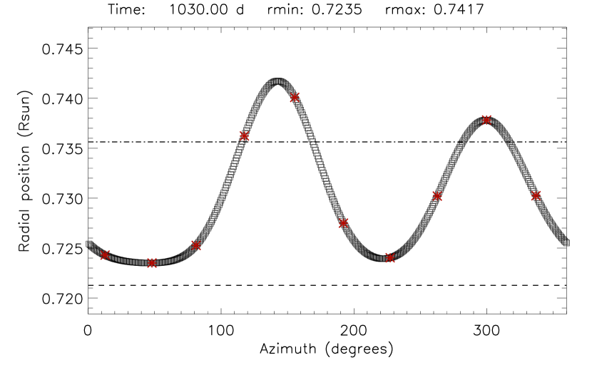
Figure 14: The shape of a flux tube with $B_{0}=7\times 10^{4}$ G, $\lambda_{0}=30^{\circ}$ and $\Delta r=5508$ km at $t=1030$ d, in the $(r,\phi)$ plane. The horizontal lines mark the boundaries of the overshoot region.

The animation files TF60.gif and TF180.gif show the evolution of a flux tube subject to a radial downflow with a duration of 60 and 120 days, respectively, until $t=300$ days (Sect. 3.2.2). Two snapshots are shown in Figs. 15 and 16, corresponding to the time when the downflow ceases in each case, i.e., at $t=60$ d and $t=180$ d. Note that for the longer-duration flow, the flux tube is radially more disturbed when the action of the downflow is finished.

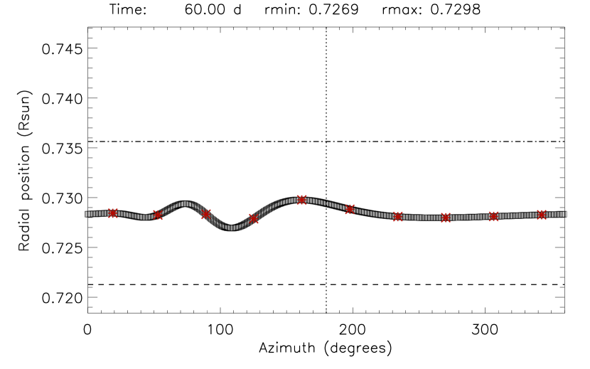
Figure 15: The shape of a flux tube with $B_{0}=7\times 10^{4}$ G, $\lambda_{0}=10^{\circ}$, at $t=60$ d, when the transient downflow ($\varv_{\rm max}=20$ m s^-1) ceases. The horizontal lines mark the boundaries of the overshoot region and the vertical line denote the azimuthal location of the centre of the downflow.

Figure 16: Same as Fig. 15, at $t=180$ d, when the transient downflow ceases.

References

- Batchelor (1967) Batchelor, G. K. 1967, Fluid dynamics (Cambridge, England, Cambridge University Press)
- Brummell et al. (2002) Brummell, N. H., Clune, T. L., & Toomre, J. 2002, ApJ, 570, 825
- Caligari et al. (1995) Caligari, P., Moreno-Insertis, F., & Schüssler, M. 1995, ApJ, 441, 886
- D’Silva & Choudhuri (1993) D’Silva, S. & Choudhuri, A. R. 1993, A&A, 272, 621
- Fan (2001) Fan, Y. 2001, ApJ, 546, 509
- Fan et al. (1994) Fan, Y., Fisher, G. H., & McClymont, A. N. 1994, ApJ, 436, 907
- Ferriz-Mas & Schüssler (1993) Ferriz-Mas, A. & Schüssler, M. 1993, Geophysical and Astrophysical Fluid Dynamics, 72, 209
- Ferriz-Mas & Schüssler (1995) Ferriz-Mas, A. & Schüssler, M. 1995, Geophysical and Astrophysical Fluid Dynamics, 81, 233
- Ferriz-Mas & Steiner (2007) Ferriz-Mas, A. & Steiner, O. 2007, Sol. Phys., 246, 31
- Holzwarth (2008) Holzwarth, V. 2008, A&A, 485, 351
- Holzwarth et al. (2007) Holzwarth, V., Schmitt, D., & Schüssler, M. 2007, A&A, 469, 11
- Moreno-Insertis (1986) Moreno-Insertis, F. 1986, A&A, 166, 291
- Moreno-Insertis et al. (1992) Moreno-Insertis, F., Schüssler, M., & Ferriz-Mas, A. 1992, A&A, 264, 686
- Schüssler (1984) Schüssler, M. 1984, A&A, 140, 453
- Schüssler (1996) Schüssler, M. 1996, in Solar and Astrophysical Magnetohydrodynamic Flows, 17–37
- Schüssler & Ferriz-Mas (2003) Schüssler, M. & Ferriz-Mas, A. 2003, in Advances in Nonlinear Dynamos, ed. A. Ferriz-Mas & M. Núñez, Taylor & Francis (London/New York), 123
- Schüssler & Ferriz Mas (2007) Schüssler, M. & Ferriz Mas, A. 2007, A&A, 463, 23
- Schüssler & Rempel (2002) Schüssler, M. & Rempel, M. 2002, in ESA Special Publication, Vol. 508, From Solar Min to Max: Half a Solar Cycle with SOHO, ed. A. Wilson, 499–506
- Shaviv & Salpeter (1973) Shaviv, G. & Salpeter, E. E. 1973, ApJ, 184, 191
- Skaley & Stix (1991) Skaley, D. & Stix, M. 1991, A&A, 241, 227
- Solanki et al. (2006) Solanki, S. K., Inhester, B., & Schüssler, M. 2006, Reports of Progress in Physics, 69, 563
- Spruit (1981) Spruit, H. C. 1981, A&A, 98, 155
- Tobias et al. (2001) Tobias, S. M., Brummell, N. H., Clune, T. L., & Toomre, J. 2001, ApJ, 549, 1183
- van Ballegooijen (1982) van Ballegooijen, A. A. 1982, A&A, 113, 99