Strange Attractors in
Dissipative Nambu Mechanics :
Classical and Quantum Aspects
Minos Axenides¹ and Emmanuel Floratos^1,2
1 Institute of Nuclear Physics, N.C.S.R. Demokritos, GR-15310, Athens, Greece
² Department of Physics, Univ. of Athens, GR-15771 Athens, Greece
axenides@inp.demokritos.gr;     mflorato@phys.uoa.gr

We extend the framework of Nambu-Hamiltonian Mechanics to include dissipation in $R^{3}$ phase space. We demonstrate that it accommodates the phase space dynamics of low dimensional dissipative systems such as the much studied Lorenz and Rössler Strange attractors, as well as the more recent constructions of Chen and Leipnik-Newton. The rotational, volume preserving part of the flow preserves in time a family of two intersecting surfaces, the so called Nambu Hamiltonians. They foliate the entire phase space and are, in turn, deformed in time by Dissipation which represents their irrotational part of the flow. It is given by the gradient of a scalar function and is responsible for the emergence of the Strange Attractors.

Based on our recent work on Quantum Nambu Mechanics, we provide an explicit quantization of the Lorenz attractor through the introduction of Non-commutative phase space coordinates as Hermitian $N\times N$ matrices in $R^{3}$. They satisfy the commutation relations induced by one of the two Nambu Hamiltonians, the second one generating a unique time evolution. Dissipation is incorporated quantum mechanically in a self-consistent way having the correct classical limit without the introduction of external degrees of freedom. Due to its volume phase space contraction it violates the quantum commutation relations. We demonstrate that the Heisenberg-Nambu evolution equations for the Quantum Lorenz system give rise to an attracting ellipsoid in the $3N^{2}$ dimensional phase space.

1 Introduction

Dissipative dynamical systems, with a low dimensional phase space, present an important class of simple non-linear physical systems with intrinsic complex behavior (homoclinic bifurcations, period doubling, onset of chaos, turbulence,…), which generated intense experimental, theoretical and numerical work in the last few decades [1, 2, 3, 4].

In this work we shall be interested to study dissipative dynamical systems with a 3-dimensional phase space from the perspective of Nambu-Hamiltonian Mechanics(NHM) [5, 6]. It represents a generalization of Classical Hamiltonian Mechanics, which is mostly appropriate for the study of phase-space volume preserving flows( Liouville’s theorem). To study dissipative systems in $R^{3}$ we generalize NHM by splitting the flow vector field into its rotational(solenoidal) and irrotational components, which we identify them to be its integrable, non-dissipative as well as dissipative parts respectively.

We apply this idea to the most famous examples of Lorenz[7] and Rössler [8] chaotic attractors which represent the prototype models for the onset of turbulence.[9, 10, 11, 12]. We present also an Euler Top deformation of the Lorenz system [13, 14] which will be a reference system for the quantization of the chaotic attractors. Following our recent work on the Quantization of NHM [15, 16] we provide a Matrix model for N-interacting Lorenz ( or Rössler) attractors. It replaces the classical three phase space coordinates by three $N\times N$ Hermitian matrices and the evolution equations with a symmetrically ordered matrix system (Weyl Quantization)[17]. As a consequence we obtain a chaotic dynamical system of $3N^{2}$ real dimensional phase space for any integer N. Finally we demonstrate that, similarly to the Lorenz system, there is an attracting ellipsoid in the $3N^{2}$-dim phase space, which provides a compact hypersurface for the localization of the higher dimensional attractors.

The plan of our paper is as follows:

In sect. 2 we introduce the framework of Dissipative Nambu-Hamiltonian Mechanics in 3-dim phase space $R^{3}$. Its Dynamics decomposes into a Non-dissipative integrable sector, which is parametrized in terms of two intersecting surfaces, the Nambu Hamiltonians (or Clebsch-Monge potentials of hydrodynamics) defined at each point of the phase space flow. One of them defines (together with the initial conditions) a two dimensional phase space embedded in $R^{3}$, while the other defines the time evolution of the system, on this curved 2d-phase space. Their intersection defines the trajectory of the system and the flow vector field. The dissipative part of the flow is the gradient of a scalar function.

In sect. 3 we apply the general framework to the Lorenz system. We isolate a conservative sector parametrized by two intersecting surfaces: a circular and a parabolic cylinder . They account, amazingly, for the double scroll topology of the full ” butterfly” attractor. As a consequence of the linear character of dissipation the trajectories of the full system get organized around the trajectories of the exactly integrable part.

The Nambu-Hamiltonian form of the integrable part, given also in terms of Poisson brackets in $R^{3}$, defines, on one of the surfaces, a two dimensional phase space (the parabolic cylinder) with a standard Poisson structure, of a quartic anharmonic oscillator of single or double potential well, depending on the initial conditions.

We present also an Euler top deformation of the Lorenz system . It is generated by a conservative sector given by the intersection of a cylinder with a paraboloid.

In sect. 4 we apply our method method of analysis to the well known case of the Rössler attractor. In this case the non-linear dissipative part distorts completely the orbits of the non-dissipative sector given by the intersection of a cylinder with an helicoid.

In sect. 5 we describe the basic steps of our Quantization prescription for Dissipative Nambu-Hamiltonian Mechanics.

In sect. 6 we construct in detail the Matrix Model for N interacting attractors as an illustration of our Quantization method. Moreover we demonstrate the existence of an attracting ellipsoid in $3N^{2}$ dim. phase space.

Finally in sect. 7 we conclude our work with the basic results and a discussion of the relevance of our proposal to the formal quantization problem of dissipation of chaotic systems[18, 19].

2 Dissipative Systems in $R^{3}$ and the Dynamics of Intersecting Surfaces

Nambu-Hamiltonian mechanics is a specific generalization of classical Hamiltonian mechanics, where the invariance group of canonical symplectic transformations of the Hamiltonian evolution equations in 2n dimensional phase space is extended to the more general volume preserving transformation group $SDiff({\cal M})$ with an arbitrary phase space manifold M of any dimension $d=\mbox{dim}({\cal M})$ .

In the present paper we will work with the case of ${\cal M}=R^{3}$, a three dimensional flat phase space manifold. Nevertheless our results could be generalized to curved manifolds of any dimension[6, 15].

Nambu-Hamiltonian mechanics of a particular dynamical system in $R^{3}$ is defined once two scalar functions $H_{i}\in C^{\infty}(R^{3}),i=1,2$, the generalized Hamiltonians [5, 6] are provided. The evolution equations are:

$$\dot{x}^{i}\ =\ \{x^{i},H_{1},H_{2}\}\ \ \ \ \ \ \ \ i=1,2,3$$ (2.1)

where the Nambu 3-bracket, a generalization of Poisson bracket in Hamiltonian mechanics, is defined as

$$\{f,g,h\}\ =\ \epsilon^{ijk}\partial^{i}f\partial^{j}g\partial^{k}h\ \ \ \ \ \ i,j,k=1,2,3\ \ \ \ \ \ \forall f,g,h\in C^{\infty}(R^{3})$$ (2.2)

Any local coordinate transformation

$$x^{i}\ \rightarrow\ y^{i}\ =\ y^{i}(x)\ \ \ \ \ \ \ \ \ i=1,2,3$$ (2.3)

which preserves the volume of phase space

$$\mbox{det}\left(\frac{\partial y^{i}}{\partial x^{j}}\right)\ =\ 1\ \ \ \ \ \forall\ x=(x^{1},x^{2},x^{3})\in R^{3}$$ (2.4)

leaves invariant the 3-bracket and therefor it is a symmetry of Nambu-Mechanics. Except for the linearity and antisymmetry of the bracket with respect to all of its arguments it also satisfies an important identity, the so called ”Fundamental identity”[FI] [6]. Let us define the operator

$${\cal L}_{(h_{1},h_{2})}\ f\ \ =\ \ \{h_{1}\ ,\ h_{2}\ ,f\ \},\ \ \ \ \ \forall\ h_{1},h_{2},f\in C^{\infty}(R^{3})$$ (2.5)

Then it can be shown that ${\cal L}$ satisfies the commutation relation

$$[{\cal L}_{(h_{1},h_{2})}\ ,\ {\cal L}_{(h_{3},h_{4})}]\ \ =\ \ {\cal L}_{\{h_{1},h_{2},h_{3}\},h_{4}}\ \ +\ \ {\cal L}_{h_{3},\{h_{1},h_{2},h_{4}\}}\ \ \ \forall\ h_{i}\in C^{\infty}(R^{3}),\ \ i=1,2,3,4$$ (2.6)

In [15] it was shown that rel(2.6) are the commutation relations of the Lie algebras of Volume preserving diffeomorphism Group SDiff($R^{3})$. The argument goes as follows: First using the operator ${\cal L}_{(H_{1},H_{2})}$ the evolution equations , rel (2.1), can be written as

$$\dot{x}^{i}\ =\ {\cal L}_{H_{1},H_{2}}\ x^{i}\ \ \ \ \ \ \ \ i=1,2,3$$ (2.7)

Given any function $f\in C^{\infty}(R^{3})$ of the phase space coordinates we obtain the Liouville eq.

$$\dot{f}\ =\ {\cal L}_{H_{1},H_{2}}\ f\ \ =\ \ \{f,H_{1},H_{2}\ \}$$ (2.8)

This equation demonstrates that $H_{1},H_{2}$ are constants of the motion and the orbit is given by the intersection of the surfaces $H_{1}^{o}=H_{1}^{o},H_{2}=H_{2}^{o}$ where

$$H_{1}^{o}\ =\ H_{1}(x_{o}^{i}),\ \ \ H_{2}^{o}\ =\ H_{2}(x_{o}^{i})$$ (2.9)

with $x^{i}_{o}$ specifying the initial conditions at $t=0$, $x^{i}_{o}=x^{i}(0)$. The formal integration of rel.(2.9) is:

$$f(x^{i}(t))\ \ =\ \ e^{t{\cal L}_{(H_{1}^{o},H_{2}^{o})}}\ \ f(x^{i}_{o})$$ (2.10)

The evolution eq.(2.1) has a flow vector field:

$$v^{i}(x)\ \ =\ \ \epsilon^{ijk}\partial^{j}H_{1}\partial^{k}H_{2}\ \ \ \ \ \ \ \ \ i,j,k=1,2,3$$ (2.11)

which is volume preserving

$$\partial^{i}v^{i}\ =\ 0$$ (2.12)

The reverse is also true. Any flow vector field of zero divergence $v^{i}\in C^{\infty}(R^{3}),\ \ i=1,2,3$ can be represented at least locally by two Clebsch-Monge potentials $H_{1},H_{2}$ [15, 20, 21, 22]

$$v^{i}\ \ =\ \ \epsilon^{ijk}\partial^{j}H_{1}\partial^{k}H_{2}$$ (2.13)

From the representation rel.(2.13) and the commutation relation for the Lie algebra of SDiff($R^{3}$) :

$$[\ {\cal L}_{u},{\cal L}_{v}\ ]\ =\ {\cal L}_{w}$$ (2.14)

where ${\cal L}_{u}=u^{i}\partial^{i}$ (similarly for $(v,w)$ with $\partial^{i}u^{i}=\partial^{i}v^{i}=0$ and

$$w^{i}\ =\ u\cdot\partial v^{i}-v\cdot\partial u^{i}$$ (2.15)

follows that $\partial^{i}w^{i}=0$ and hence the commutation relations (2.6) follow. We will name the phase-space volume preserving flows ”Non-dissipative” while the non-conserving ones ”Dissipative”.

The general flow vector fields will have regions $D_{+}\subset R^{3}$ with

$$\partial^{i}v^{i}(x)>0\ \ \ \ x\in D_{+}$$ (2.16)

where any volume element is expanded by the flow and regions $D_{-}\subset R^{3}$, $D_{+}\cap D_{-}=0$ with

$$\partial^{i}v^{i}(x)\ <\ 0\ \ \ \ \ \ \ \forall x\in D_{-}$$ (2.17)

where the volume elements are contracted.

The standard local stability analysis of the flow, involves the determination of the critical points $x^{i}_{o}$(equilibrium points) where $v^{i}(x_{o})=0,\ \ i=1,2,3$, as well as the examination of the eigenvalues of the fluctuation matrix ($\partial^{i}v^{j}),{i,j}=1,2,3$) at the critical points which characterize the phase space portrait of the flow.

Under variations of external parameters (environment) the location and stability character of the critical points vary. There arises possibilities of Hopf bifurcations, transition to chaos, turbulence etc [1, 2, 3, 4, 9].

In order to bring into play the Nambu-Hamiltonian Mechanics framework we firstly generalize it for general dissipative systems in $R^{3}$ phase space. We will decompose any flow vector field into its rotational and irrotational parts.

$$v^{i}\ =\ \epsilon^{ijk}\partial^{j}A^{k}+\partial^{i}D\ \ \ \ \ \ \ \ i,j,k=1,2,3$$ (2.18)

with the vector potential determined up to a local gauge transformation:

$$A^{i}\ \rightarrow\ A^{i}\ +\ \partial^{i}\Lambda\ \ \ \ \ \ \ i=1,2,3$$ (2.19)

and

$$\partial^{i}v^{i}\ =\ \nabla^{2}D$$ (2.20)

Given $\partial^{i}v^{i}$ and appropriate BC we can , in principle, determine the dissipation function D.

In general D is determined up to harmonic functions on $R^{3}$. Since the rotational component is divergenceless, we shall call it the Non-dissipative part of the flow (ND), $\vec{v}_{ND}$ while the irrotational component we will identify it with the Dissipative part(D), $\vec{v}_{D}$. Once the vector potential $A^{i}$ has been determined we can choose the Clebsch-Monge gauge where [CM]:

$$A^{i}\ \ =\ \ H_{1}\partial^{i}H_{2}$$ (2.21)

utilizing two ”generalized Hamiltonians” or equivalently Clebsch-Monge flow potentials. The flow equations take the form

$$\dot{x}^{i}\ =\ \{x^{i},H_{1},H_{2}\}\ +\ \partial^{i}D\ \ \ \ \ \ \ \ \ i=1,2,3$$ (2.22)

and in vector form

$$\dot{\vec{x}}\ \ =\ \ \vec{\nabla}H_{1}\times\vec{\nabla}H_{2}+\vec{\nabla}D$$ (2.23)

We notice that given a pair of functions $H_{1},H_{2}$ such that

$$\vec{v}_{ND}\ \ =\ \ \vec{\nabla}H_{1}\times\vec{\nabla}H_{2}$$ (2.24)

any transformation of $H_{1},H_{2}$

$$H_{i}\rightarrow H_{i}^{\prime}(H_{1},H_{2})\ \ \ \ \ i=1,2$$ (2.25)

with unit Jacobian

$$\mbox{det}\left(\frac{\partial H_{i}^{\prime}}{\partial H_{j}}\right)\ =\ 1$$ (2.26)

gives also

$$\vec{v}_{ND}\ =\ \vec{\nabla}H_{1}^{\prime}\times\vec{\nabla}H_{2}^{\prime}$$ (2.27)

Although the geometrical power of the surfaces $H_{1},H_{2}$ in the Nambu mechanics framework ($D=0$) is lost, still there are interesting cases to consider. First the generalized Hamiltonians are not conserved but we have

$$\dot{H_{1}}\ = \ \vec{\nabla}\vec{D}\cdot\vec{\nabla}H_{1}$$

$$\dot{H_{2}}\ = \vec{\nabla}D\cdot\vec{\nabla}H_{2}$$ (2.28)

and for D we obtain the equations:

$$\dot{D}\ =\ (\vec{\nabla}D)^{2}\ +\ \{D,H_{1},H_{2}\}$$ (2.29)

if the relative orientation of the surfaces is fixed of positive sign, we get $\{D,H_{1},H_{2}\}>0$ and D increasing for all times. In general this is not true.

We also see that if D is a surface orthogonal to either $H_{1}$ or $H_{2}$ then the latter are conserved. If D is orthogonal to both surfaces, then it must be parallel to $\vec{\nabla}H_{1}\times\vec{\nabla}H_{2}$ and the orbit of the dynamical system (2.24) is again the intersection of $H_{1}$ and $H_{2}$ surfaces which are both conserved.

The decomposition of a general phase space flow vector field in its (ND) and (D) parts may help to understand qualitatively the phase space portrait behavior of the full system. Indeed, in principle, it is possible to solve explicitly for the phase-space trajectories of the ND part

$$\dot{\vec{x}}\ =\ \vec{v}_{ND}\ =\ \vec{\nabla}\ H_{1}\times\vec{\nabla}\ H_{2}$$ (2.30)

using the two integrals of motion

$$H_{i}(\vec{x})\ =\ H_{i}(\vec{x}_{o})\ \ \ \ \ \ \ i=1,2$$ (2.31)

By parametrizing their intersection we can specify the explicit time dependence of the motion.

In ref.[15] we reduced the evolution equation of the form (2.32) Nambu Mechanics in Hamiltonian-Poisson form as follows:

$$\dot{x}^{i}\ =\ \{x^{i},H_{1},\}_{H_{2}}$$ (2.32)

where the induced Poisson bracket

$$\{f,g\}_{H_{2}}\ =\ \epsilon^{ijk}\partial^{i}f\partial^{j}g\partial^{k}H_{2}$$ (2.33)

satisfies all the required properties like linearity, antisymmetry and the Jacobi identity:

$$\{\{f,g\}_{H_{2}},h\}_{H_{2}}+\{\{g,h\}_{H_{2}},f\}_{H_{2}}\ +\ \{\{h,f\}_{H_{2}},g\}_{H_{2}}\ =\ 0$$ (2.34)

The Jacobi identity follows from the Fundamental Identity rel.(2.7).

Since $H_{2}$ is conserved it defines a fixed surface ${\Sigma}_{2}:H_{2}=H_{2}(\vec{x}_{o})$ embedded in $R^{3}$ which can be considered as a two dimensional phase space. In certain cases we may find explicit local or global parametrization of $H_{2}$ with two parameters, $(u,v)\in{\Delta}\subset R^{2}$:

$$x^{i}\ =\ x^{i}(u,v)\ \ \ \ \ \ \ (u,v)\in\Delta\ \ \ \ i=1,2,3$$ (2.35)

such that $(x^{i})\in\Sigma_{2}$

$$H_{2}(x^{i}(u,v))\ =\ H_{2}(\vec{x}_{o})$$ (2.36)

The orbits on the $\Sigma_{2}$ phase-space are determined by the Hamiltonian $H_{1}$ :

$$\dot{x}^{i}\ \ =\ \ \{x^{i},H_{1}\}_{\Sigma_{2}}\ \ \ \ \ \ \ \ \ i=1,2,3$$ (2.37)

Comparing the relations on $\Sigma_{2}$

$$\dot{\vec{x}}\ \ =\ \ \vec{x}_{u}\dot{u}\ +\ \vec{x}_{v}\dot{v}$$ (2.38)

and

$$\dot{\vec{x}}\ =\ \vec{\nabla}H_{1}\times\vec{\nabla}H_{2}$$ (2.39)

we get:

$$\dot{u}\ \cdot\ (\vec{x}_{u}\times\vec{x}_{v})\ =\ \vec{\nabla}H_{2}\ \cdot\ \partial_{v}H_{1}$$ (2.40)

$$\dot{v}\ \cdot\ (\vec{x}_{u}\times\vec{x}_{v})\ =\ -\vec{\nabla}H_{2}\ \cdot\ \partial_{u}H_{1}$$ (2.41)

Since $\vec{x_{u}}\times\vec{x_{v}}$ and $\vec{\nabla}H_{2}$ are normal and collinear at every point of $\Sigma_{2}$ using parameters $u,v$ of the same orientation (outwards) we must have:

$$\vec{x}_{u}\times\vec{x}_{v}\ =\ \rho(u,v)\ \ \vec{\nabla}H_{2}$$ (2.42)

for a positive function $\rho(u,v)$ on $\Sigma_{2}$, we thus get from rel.(2.40-2.42)

$$\dot{u}\ =\ \frac{1}{\rho(u,v)}\ \ \partial_{v}\ H_{1}$$ (2.43)

$$\dot{v}\ =\ -\frac{1}{\rho(u,v)}\ \ \partial_{u}\ H_{1}$$ (2.44)

Relations $(2.43-2.44)$ can be written as Hamilton-Poisson eqs on $\Sigma_{2}$ :

$$\dot{u}\ =\ \{u,H_{1}\}_{\Sigma_{2}}$$ (2.45)

$$\dot{v}\ =\ \{v,H_{1}\}_{\Sigma_{2}}$$ (2.46)

with the Poisson bracket on $\Sigma_{2}$:

$$\{f,g\}_{\Sigma_{2}}\ =\ \frac{1}{\rho(u,v)}\ (\partial_{u}f\partial_{v}g\ -\ \partial_{u}g\partial_{v}f)$$ (2.47)

We shall use instead the level-set Morse functions $H_{2}$ for the phase space surfaces, because it is not always easy to find appropriate surface parametrizations.

We observe that from eq.(2.33), the Poisson structure of the $H_{2}$ phase-space, is described in the algebra of phase space coordinates $x^{i}$ :

$$\{x^{i},x^{j}\}_{H_{2}}\ \ =\ \ \epsilon^{ijk}\partial^{k}H_{2}$$ (2.48)

which is preserved by the eqns. of motion of the ND part. As an example of Nambu-Hamiltonian dynamics and the reduced Hamilton-Poisson form, we will consider the Euler free Top [5, 15].

For the Euler free top there are two conserved quantities. The total angular momentum squared:

$$H_{2}\ =\ \frac{1}{2}\ \left(l_{1}^{2}\ +\ l_{2}^{2}\ +\ l_{3}^{2}\right)$$ (2.49)

and the energy:

$$H_{1}\ =\ \frac{1}{2}\ \left(\frac{l_{1}^{2}}{I_{1}}\ +\ \frac{l_{2}^{2}}{I_{2}}\ +\ \frac{l_{3}^{2}}{I_{3}}\right)$$ (2.50)

where $(l_{i}),i=1,2,3$ are the components of the angular momentum, in the body frame, and $I_{1},i=1,2,3$ are the eigenvalues of the moments of inertia tensor. The Nambu-Hamilton eqns :

$$\dot{l_{i}}\ \ =\ \ \{l_{i},H_{1},H_{2}\}\ =\ \epsilon^{ijk}\partial^{j}H_{1}\partial^{k}H_{2}$$ (2.51)

provide the correct eqs. of motion for the rigid body :

$$\dot{l_{1}}\ = \ (\frac{1}{I_{2}}-\frac{1}{I_{3}})l_{2}l_{3}\ \ \ \ \$$

$$\dot{l_{2}}\ = \ (\frac{1}{I_{3}}-\frac{1}{I_{1}})l_{3}l_{1}\ \ \ \ \$$

$$\dot{l_{1}}\ = \ (\frac{1}{I_{1}}-\frac{1}{I_{2}})l_{1}l_{2}$$ (2.52)

The 2d-phase space is determined by the initial conditions:

$$l_{1}^{2}(t)+l_{2}^{2}(t)+l_{3}^{2}(t)\ =\ 2H_{2}\ =\ l_{o}^{2}=l_{1,o}^{2}+l_{2,o}^{2}+l_{3,o}^{2}$$ (2.53)

which is an $S^{2}$ sphere in $R^{3}$.

The induced Poisson structure of the coordinates in $R^{3}$ is:

$$\{l_{i},l_{j}\}_{S^{2}}\ \ =\ \ \epsilon_{ijk}\partial_{k}H_{2}=\epsilon_{ijk}l_{k}\ \ \ \ \ \ \ \ \ \ \ \ \ \ \ \ \ i,j,k=1,2,3$$ (2.54)

the Poisson $SO(3)$ algebras and eqs. (2.52) can be written

$$\dot{l}_{i}\ \ =\ \ \{l_{i},H_{1}\}_{S^{2}}\ \ \ \ \ \ \ \ \ i=1,2,3$$ (2.55)

In the following sections we are going to present a detailed investigation of the Lorenz and Rössler attractors from the point of view of Dissipative Nambu-Hamiltonian Dynamics.

3 The Lorenz System and its Euler top Deformation

3.1 Lorenz Attractor from Dissipative Nambu Dynamics .

The Lorenz model was invented as a three Fourier mode truncation (Gallerkin approximation [3] of the basic eqs. for heat convection in fluids in Reyleigh-Benard type of experiments [23, 24, 25] The time evolution eqns. in the space of three Fourier modes $x,y,z$ which we identify as phase-space are :

$$\dot{x}\ = \ \sigma(y-x)$$

$$\dot{y}\ = \ x(r-z)-y$$

$$\dot{z}\ = \ xy-bz$$ (3.1)

where $\sigma$ is the Prandtl number, r is the relative Reynolds number and b the geometric aspect ratio .

The standard values for $\sigma$, b are $\sigma=10,b=\frac{8}{3}$ with r taking values in $1\leq r<\infty$. There are dramatic changes of the system as r passes through various critical values which follow the change of stability character of the three critical points of the system $P_{1}$ : $x=y=z=0,P_{\pm}:x=y=\pm\sqrt{b(r-1)},z=r-1$

Lorenz discovered the non-periodic deterministic chaotic orbit for the value $r=28$, which is today identified as a Strange Attractor with a Hausdorff dimension of ($d=2.06$)[26]. Standard reference for an exhaustive numerical investigation of the Lorenz system is the book by Sparrow [27], although there is an extended list of numerical and analytic work on the system. For a qualitative discussion of the physics we refer to [7, 11, 12].

We can have a first glimpse of the geometry of motion, for a volume element in flow under eq.(3.1), if we cast the Lorenz system in Matrix form as follows:

$$\frac{d}{dt}\left(\begin{array}[]{c}x\\ y\\ z\end{array}\right)\ =\ \left(\begin{array}[]{ccc}-\sigma&\sigma&0\\ r&-1&-x\\ 0&x&-b\end{array}\right)\left(\begin{array}[]{c}x\\ y\\ z\end{array}\right)\ \equiv\ A\left(\begin{array}[]{c}x\\ y\\ z\end{array}\right)$$ (3.2)

and decompose the matrix A into its symmetric and antisymmetric parts $A=A_{s}+A_{as}$ :

$$A_{s}\ =\ \left(\begin{array}[]{ccc}-\sigma&\frac{\sigma+r}{2}&0\\ \frac{\sigma+r}{2}&-1&0\\ 0&0&-b\end{array}\right)$$ (3.3)

$$A_{as}\ =\ \left(\begin{array}[]{ccc}0&\frac{\sigma-r}{2}&0\\ \frac{r-\sigma}{2}&0&-x\\ 0&x&0\end{array}\right)$$ (3.4)

The matrix $A_{s}$ executes an expansion along an axis $x^{\prime}$, a contraction along the orthogonal $y^{\prime}$ axis, as well as a contraction along the z-axis. The antisymmetric matrix $A_{as}$ executes a rotation around z-axis with a constant $\frac{r-\sigma}{2}$ angular velocity and a rotation around x-axis with an x dependent angular velocity.

The axes $x^{\prime},y^{\prime}$ are rotated fixed axes which we find through a diagonalization of $A_{s}$. We have thus the basic qualitative mechanism for chaos through stretching, twisting and folding [4, 9, 11] .

We turn our attention now to an important characteristic property of the Lorenz attractor system, i.e. its ”Orbit localizability” within an attracting(trapping) ellipsoid.[7]

Consider the ellipsoid in $R^{3}$:

$$S_{1}\ =\ rx^{2}+\sigma y^{2}+\sigma(z-2r)^{2}$$ (3.5)

Along the orbits we have

$$\frac{dS_{1}}{dt}\ =\ \dot{\vec{r}}\cdot\vec{\nabla}S_{1}\ =\ -2\sigma\ [rx^{2}\ +\ y^{2}+\ b(z-r)^{2}\ -\ br^{2}]$$ (3.6)

If we consider fixed values of $S_{1}$ such that the corresponding ellipsoid $S_{1}=\mbox{constant}$ lies entirely outside the fixed ellipsoid

$$S_{2}:\ \ \ \ rx^{2}+y^{2}\ +\ b(z-r)^{2}\ =\ br^{2}$$ (3.7)

then we get

$$\dot{\vec{r}}\cdot\vec{\nabla}S_{1}\ \ <\ \ 0$$ (3.8)

for all orbits intersecting $S_{1}$, i.e. all of them are ingoing to the surface. We observe that $S_{2}$ acts like an attractor region. There have been various attempts made to localize the Lorenz attractor, by convex surfaces, in order to get information about Hausdorff dimensions [26] and other characteristics [24, 28].

The case of Rössler attractor has been studied also from this point of view[30].

We will deal with the issue of Localization and the existence of an attracting ellipsoid in our Matrix Model generalization of the Lorenz systems, in order to get attracting ellipsoids in higher dimensional phase spaces.

Concerning analytical methods we observe that the system can be explicitly integrated out, through the use of Liouville operator. For any observable $\rho(x,y,z)$ on $R^{3}$ we get the time evolution on trajectories

$$\dot{\rho}\ =\ {\cal L}\cdot\rho$$ (3.9)

with

$${\cal L}\ =\ \sigma(y-x)\partial_{x}\ +\ [x(r-z)-y]\partial_{x}\ +\ (xy-bz)\partial_{z}$$ (3.10)

The formal solution for the x-coordinates is $({\cal L}_{o}={\cal L}(x_{o},y_{o},z_{o}))$ :

$$x(t)\ =\ e^{t{\cal L}_{o}}x_{o}$$ (3.11)

Similarly for y and z respectively. Since the trajectories are smooth and bounded, we must have convergent Taylor series in time[25, 31, 32]:

$$x(t)\ =\ \sum^{\infty}_{k=0}x_{k}\frac{t^{k}}{k!}$$ (3.12)

with

$$x_{k}\ =\ (\frac{d}{dt})^{k}x(t)\mid_{t=0}\ \ \ \ \ k=0,1,2,\cdots$$ (3.13)

From rel(3.11) we get

$$x_{k}\ =\ {\cal L}^{k}_{o}\ x_{o}\ \ \ \ \ \ \ \ \ \ \ k=0,1,2,\cdots$$ (3.14)

So we can get as many coefficients $x_{k}$ we like by simply looking at the linear in the derivatives $\partial_{x_{o}},\partial_{y_{o}},\partial_{z_{o}}$, part of ${\cal L}^{k}_{o}$.

We now proceed to describe the Lorenz system in the framework of section 2. The flow vector field $\vec{v}$ is analyzed into its dissipative and non-dissipative parts as follows:

$$\vec{v}_{D}\ =\ (-\sigma x,-y,-bz)\ =\ \vec{\nabla}D$$ (3.15)

with the ”Dissipation” function

$$D\ =\ -\frac{1}{2}\ (\sigma x^{2}\ +\ y^{2}\ +\ bz^{2})$$ (3.16)

and

$$\vec{v}_{ND}\ =\ (\sigma y,x(r-z),xy)\ =\ (0,y,z-r)\times(-x,0,\sigma)$$ (3.17)

From rel (3.17) we get the two Hamiltonians or Clebsch-Monge potentials $H_{1},H_{2}$

$$\vec{\nabla}H_{1}\times\vec{\nabla}H_{2}\ =\ \vec{v}_{ND}$$ (3.18)

or

$$H_{1}\ =\ \frac{1}{2}[y^{2}+(z-r)^{2}]$$ (3.19)

and

$$H_{2}\ =\ \sigma z\ -\ \frac{x^{2}}{2}$$ (3.20)

The Lorenz system (3.1) can thus be written in the form ( $\vec{r}=(x,y,z)$):

$$\dot{\vec{r}}\ =\ \vec{\nabla}H_{1}\times\vec{\nabla}H_{2}\ +\ \vec{\nabla}D$$ (3.21)

In the Non-Dissipative part(ND) of the dynamical system

$$\dot{\vec{r}}\ =\ \vec{\nabla}H_{1}\times\vec{\nabla}H_{2}$$ (3.22)

the Hamiltonians $H_{1},H_{2}$ are conserved and their intersection defines the ND orbit. Moreover if we get the reduced Poisson structure (sect.2) from $H_{2}$ we obtain the 2-dim phase space $\Sigma_{2}$ to be the family of parabolic cylinders with symmetry axis the y-axis:

$$H_{2}=\mbox{constant}=H_{2}(\vec{r_{o}})$$ (3.23)

$\Sigma_{2}$ is thus given by

$$z\ =\ z_{o}+\frac{x^{2}-x_{o}^{2}}{2\sigma}$$ (3.24)

with $x_{o},z_{o}$ the initial condition for $x,z$. The induced Poisson algebra (rel. 2.33) is given by

$$\{x,y\}_{H_{2}}\ = \ \partial_{z}H_{2}\ =\sigma$$

$$\{y,z\}_{H_{2}}\ = \ \partial_{x}H_{2}\ =-x$$

$$\{z,x\}_{H_{2}}\ = 0$$ (3.25)

The dynamics on the 2d-phase space $\Sigma_{2}$ is given by $H_{1}$

$$\dot{x}\ = \ \{x,H_{1}\}_{H_{2}}\ \ \ \$$

$$\dot{y}\ = \ \ \{y,H_{1}\}_{H_{2}}$$

$$\dot{z}\ = \ \ \{z,H_{1}\}_{H_{2}}$$ (3.26)

and $H_{1}$ is an anharmonic oscillator Hamiltonian with $(x/\sigma,y)$ conjugate canonical variables. Using rel.(3.19-3.20) we get on $\Sigma_{2}$:

$$H_{1}\ =\ \frac{1}{2\sigma^{2}}\ [y^{2}\ +\ \frac{1}{2}\ (x^{2}\ -\ a^{2})^{2}]$$ (3.27)

with

$$a^{2}\ =\ x_{o}^{2}\ -\ 2\sigma(z_{o}\ -\ r)\ =\ -2H_{2}\ +\ 2\sigma r$$ (3.28)

where $\frac{1}{\sigma^{2}}$ plays the role of the mass. Depending on the initial conditions we may have a single well $(a^{2}\leq 0,H_{2}\geq\sigma r)$ or a double well potential ( $a^{2}>0,H_{2}<\sigma r$ ) respectively. The trajectories , the intersections of the two cylinders , $H_{1}$ and $H_{2}$ with orthogonal symmetry axes $(x,y)$ may either have one lobe left/right or may be running from the right to the left lobe. This is reminiscent of the topology structure of the orbits of the Lorenz chaotic attractor.

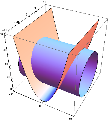
Figure 1: Intersecting surfaces for Lorenz Attractor

In fig.1 we present the Lorenz Intersecting surfaces for initial values $x_{0}=z_{0}=0,y_{0}=1$. So the orbits of the non-dissipative system are the seeds around which and through the action of dissipation, the actual attractor is organized. In fig.2 we present such an example for orbits of the nondissipative sector of the lorenz system superimposed with the full Lorenz attractor for the same initial conditions and standard values of the parameters ( $\sigma=10,r=28,b=8/3$).

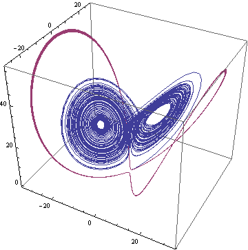
Figure 2: Nondissipative Orbit and Lorenz Attractor

We may observe directly the action of dissipation. Similar observations have been made by Haken, in a different physics context and Nevir-Blender [33, 34] without use of the induced Poisson structure in $R^{3}$ rel.(3.25) and the ensuing interpretation [15] (rel.3.26) Sparrow has analyzed the integrable non-dissipative system, adding perturbative dissipative terms [27].

The full Lorenz system does not conserve $H_{1},H_{2}$ and there is a random motion of the two surfaces against each other. Their intersection is time varying. In effect at every moment the system jumps from periodic to periodic orbit of the non-dissipative sector. Moreover the motion of the non-dissipative system around the two lobes, either left or right, can now jump from time to time from one lobe to the other.

We would like to mention at this point ,another interesting feature of the Lorenz system. Due to the linear character of the dissipative part of the Lorenz attractor ,we are able to transform the full system to a volume preserving flow with time dependent generalized Hamiltonians ( or equivalently intersecting surfaces).

This is done as follows. For a general Nambu-Hamiltonian system with linear dissipation:

$$\dot{x}\ = \ (\vec{\nabla}H_{1}\times\vec{\nabla}H_{2})_{1}\ -\ \alpha x\ \ \ \$$

$$\dot{y}\ = \ (\vec{\nabla}H_{1}\times\vec{\nabla}H_{2})_{2}\ -\ \beta y\ \ \ \$$

$$\dot{z}\ = \ \vec{\nabla}H_{1}\times\vec{\nabla}H_{2})_{3}\ -\ \gamma z$$ (3.29)

we define new variables (comoving frame) :

$$x=e^{-\alpha t}u\ \ ,\ \ y=e^{-\beta t}v\ \ ,\ \ z=e^{-\gamma t}w$$ (3.30)

Using the gradient operators with respect to $\vec{q}=(u,v,w)$ we can check that the eqs. of motion (3.29) become

$$e^{-(\alpha+\beta+\gamma)t}\frac{d}{dt}(u,v,w)\ =\ \vec{\nabla}_{\vec{q}}H_{1}\times\vec{\nabla}_{\vec{q}}H_{2}$$ (3.31)

where

$$H_{i}\ =\ H_{i}(e^{-\alpha t}u,e^{-\beta t}v,e^{-\gamma t}w)\ \ \ \ \ \ i=1,2$$ (3.32)

Eq.(3.31) implies that the $(u,v,w)$ phase space volume elements are conserved. In effect, we have a new time variable $\tau\ =\ \frac{1}{\alpha+\beta+\gamma}e^{(\alpha+\beta+\gamma)t}$

$$\frac{d}{dt}(u,v,w)\ =\ \vec{\nabla}_{\vec{q}}H_{1}\times\vec{\nabla}_{\vec{q}}H_{2}$$ (3.33)

The Lorenz attractor can be brought to the form of rel.(3.33). In terms of our Hamiltonian reduction it is a Hamiltonian system with a time dependent Hamiltonian $H_{1}(e^{-\sigma t}u,e^{-t}v,e^{-bt}w)$ on a dynamical two dimensional phase space which is defined by the surface $H_{2}(e^{-\sigma t}u,e^{-t}v,e^{-bt}w)=\mbox{constant}$ which moves in $R^{3}$. In the comoving coordinates $u,v,w$ the evolution of the system is volume preserving. A direct way to see the time dependence of $H_{1},H_{2}$ and D, is through their time evolution eqs. 2.28-2.29. For the Lorenz attractor system we have

$$H_{1} = \frac{1}{2}\ \ (y^{2}+(z-r)^{2})\ \ \ \ \ \ \ \ \ \$$

$$H_{2} = \sigma z\ -\ \frac{x^{2}}{2}\ \ \ \ \ \ \ \ \$$

$$D = \ \ -\frac{1}{2}\ \ (\sigma x^{2}\ +\ y^{2}\ +\ bz^{2})$$ (3.34)

Their normal vectors are respectively:

$$\vec{\nabla}H_{1}\ = \ (0,y,z-r)\ \ \ \ \ \ \ \ \$$

$$\vec{\nabla}H_{2}\ = \ (-x,0,\sigma)\ \ \ \ \ \ \$$

$$\vec{\nabla}D\ = \ (-\sigma x,-y,-bz)$$ (3.35)

Finally we get:

$$\dot{H}_{1}\ = \ -y^{2}-bz\ (z-r)\ \ \ \ \ \ \ \$$

$$\dot{H}_{2}\ = \ \sigma x^{2}-\sigma bz\ \ \ \ \ \$$

$$\dot{D}\ = \ \sigma^{2}x^{2}+y^{2}+b^{2}z^{2}-(\sigma+r)\ xy+(1-b)\ xyz$$ (3.36)

Since the Lorenz attractor is bounded in phase-space, the coordinates $x,y,z$ have maxima and minima, which implies that the surfaces $H_{1},H_{2},S$ have maximum and minimum positions. So the Lorenz attractor is bounded by the volume enclosed by the maximum and minimum positions of these three surfaces. Estimates of the maximum and minimum values of the functions $H_{1},H_{2}$ have been determined using the constraint of the bounding Lorenz ellipsoid as well as other surfaces.

Closing we would like to point out that our analysis of the Lorenz system applies equally to similar dissipative systems in $R^{3}$ such as the Chen [29] and the Leipnik-Newton [13] strange attractor constructions. They all share the same structure with the Lorenz system. It involves a nonlinear, nondissipative, integrable part which admits an intersecting surface Nambu parametrization superimposed to a linear dissipative sector. Last but not least it should be remarked that the $R^{3}$ geometrical picture presented above is directly generalizable to dissipative systems with $R^{2n+1}$ phase space dynamics. In complete analogy it is expected that $2n$ intersecting surfaces (Nambu Hamiltonians) generate the integrable sector of the system.

3.2 A Strange Rigid Body Attractor as Dissipative Dynamics of Intersecting Paraboloid with a Cylinder

We notice, in passing, that we can obtain a dissipative Euler top deformation of the Lorenz system, through the addition of terms rel.(2.55) :

$$\dot{l}^{i}\ =\ \{l^{i},H_{1}\}_{S^{2}}\ +\ \partial^{i}D\ \ \ \ \ \ \ \ \ i=1,2,3$$ (3.37)

Indeed as we can see, the Lorenz attractor system

$$\dot{l}^{1}\ = \ \sigma(l^{2}-l^{1})\ \ \ \ \ \$$

$$\dot{l}^{2}\ = \ l^{1}(r-l^{3})-l^{2}\ \ \ \ \ \$$

$$\dot{l}^{3}\ = \ l^{1}l^{2}-bl^{3}$$ (3.38)

can be written as a dissipative Euler Top through the choice $I_{2}=I_{3}=I$ for any $I>0$ and $I_{1}=\frac{I}{1+I}$ but only for the special relation $\sigma=r$ of its free parameters $\sigma,r$. The corresponding Dissipation function D is given by:

$$D\ =\ -\sigma l^{1}l^{2}\ +\ \frac{1}{2}\ [\sigma(l^{1})^{2}+(l^{2})^{2}+(l^{3})^{2}]$$ (3.39)

The last condition $\sigma=r$, comes about from the constraint that we add to the Euler top non-dissipative flow, $\vec{v}_{ND}=(0,-l^{1}l^{3},l^{1}l^{2})$, an irrotational (gradient) flow :

$$\vec{v}_{D}=(\sigma(l^{2}-l^{1}),rl^{1}-l^{2},-bl^{3})$$ (3.40)

with the condition,

$$\vec{\nabla}\times\vec{v}_{D}\ =\ (0,0,r-\sigma)\ =\ \vec{0}$$ (3.41)

We performed some numerical experiments for the values of $\sigma=r$. We find that there is a chaotic attractor for values $\sigma=r=(25,26,27)$ and $b=8/3$.

We introduce now, to a 2-parameter Euler top deformation of the Lorenz system

$$\dot{l}_{1}\ = \ \left(\frac{1}{I_{2}}\ -\ \frac{1}{I_{3}}\right)l_{2}l_{3}\ +\ \sigma(l_{2}-l_{1})\ \ \ \ \ \$$

$$\dot{l}_{2}\ = \ \left(\frac{1}{I_{3}}\ -\ \frac{1}{I_{1}}\right)l_{1}l_{3}\ +\ rl_{1}-l_{2}\ \ \ \ \ \$$

$$\dot{l}_{3}\ = \ \left(\frac{1}{I_{1}}\ -\ \frac{1}{I_{2}}\right)l_{1}l_{2}\ -\ bl_{3}$$ (3.42)

where we have chosen $I_{3}\geq I_{2}>I_{1}$. For more general linear terms we obtain the Leipnik-Newton linear control system on the motion of a Rigid Body where for appropriate values of the coefficients a double Lorenz attractor is obtained [13].

Performing a similar decomposition in a conservative(non-dissipative) and dissipative sectors of our system we get

$$\vec{v}_{ND}\ =\ \left((\frac{1}{I_{2}}-\frac{1}{I_{3}})l_{2}l_{3}+\sigma l_{2},(\frac{1}{I_{3}}-\frac{1}{I_{1}})l_{1}l_{3}+rl_{1},(\frac{1}{I_{1}}-\frac{1}{I_{2}})l_{1}l_{2}\right)$$ (3.43)

and

$$\vec{v}_{D}\ =\ (-\sigma l_{1},-l_{2},-bl_{3})$$ (3.44)

we can find two Hamiltonians $H_{1},H_{2}$ and the Dissipation function D:

$$\vec{\nabla}H_{1}\times\vec{\nabla}H_{2}\ = \ \vec{v}_{ND}$$

$$\vec{\nabla}D=-(\sigma l_{1},l_{2},bl_{3})$$ (3.45)

In order to get the two characteristic lobes of the attractor already at this level we notice that we can write the non-dissipative flow of rel.(3.43) as :

$$\vec{v}_{ND}\ =\ (0,\beta l_{2},\gamma l_{3}-r)\times(-l_{1},\delta l_{2},\sigma^{\prime})$$ (3.46)

where

$$\beta=\frac{1}{I_{1}}-\frac{1}{I_{2}}\ ,\ \gamma=\frac{1}{I_{1}}-\frac{1}{I_{3}}\ ,\ \delta=\frac{1-I_{2}/I_{3}}{1-I_{2}/I_{1}}$$ (3.47)

and

$$\sigma^{\prime}\ =\ \frac{\sigma-\delta r}{\beta}$$ (3.48)

From rel(3.46) we get,

$$H_{1}\ =\ \frac{1}{2}\ [\beta l_{2}^{2}\ +\ (\gamma l_{3}-r)^{2}]$$ (3.49)

an elliptic cylinder along the $l_{1}$ axis and

$$H_{2}=\sigma^{\prime}l_{3}-\frac{l_{1}^{2}}{2}\ +\ \delta\frac{l_{2}^{2}}{2}$$ (3.50)

a paraboloid with elliptic cross section. The Dissipation function D is identical to the case of the Lorenz attractor:

$$D\ =\ -\frac{1}{2}(\sigma l_{1}^{2}+l_{2}^{2}+bl_{3}^{2})$$ (3.51)

From the chosen ordering $I_{3}\geq I_{2}>I_{1},$ we get $\beta>0,\delta\leq 0$ ($=0$ Lorenz case ) and $\sigma^{\prime}>0$. The $H_{2}$, an elliptic paraboloid is oriented towards the positive $l_{3}$ axis. The intersection of the two surfaces $H_{1},H_{2}$ accounts for the existence of the two lobes of the attractor. Depending on the initial conditions it is possible that these lobes are connected with trajectories of the non-dissipative system. In fig.3 we present the intersecting surfaces for the Euler- Lorenz nondissipative system for the initial values $x_{0}=z_{0}=0,y_{0}=1$ and values of the parameters $\sigma=10,r=28,b=8/3,I_{1}=1,I_{2}=2,I_{3}=3$.

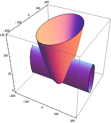
Figure 3: Intersecting surfaces for Euler Top Attractor

A detailed analysis with numerical experiments will be presented in a forthcoming publication. In fig.4 we present the nondissipative orbit for Euler-Lorenz system superimposed with its full strange attractor for the same set of initial conditions and parameters as in fig.3.

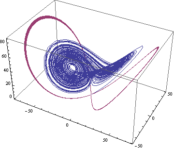
Figure 4: Nondissipative orbit and Euler-Lorenz Attractor

4 Rössler Attractor from Dissipative Dynamics of a Cylinder Intersecting with an Helicoid

Rössler introduced a simpler than Lorenz’s nonlinear ODE system with a 3d- phase space, in order to study in more detail the characteristics of chaos, which is motivated by simple chemical reactions [8].

The Rössler system is given by the evolution eqns:

$$\dot{x}\ = \ -y-z$$

$$\dot{y}\ = \ x+ay$$

$$\dot{z}\ = \ b+z(x-c)$$ (4.1)

with parameters $a,b,c$ usually taking standard values $a=b=0.2,c=5.1$ or $a=b=0.1,c=14$ for the appearance of the chaotic attractor. The two fixed points of the system are:

$$F_{\pm}:(x_{\pm},y_{\pm},z_{\pm})=(\frac{c\pm\sqrt{c^{2}-4ab}}{2},-\frac{c\pm\sqrt{c^{2}-4ab}}{2a},\frac{c\pm\sqrt{c^{2}-4ab}}{2a})$$ (4.2)

and depending on the parameters $a,b,c$ their stability character changes. For the standard values both are unstable saddle points with the $F_{-}$ having an unstable 2d manifold whereas the $F_{+}$ an unstable 1d manifold. Studying the Poincare maps in the x-plane and the bifurcation diagrams for $y_{n+1}=f(y_{n})$ return map, one discovers the period doubling bifurcations to be the underlying mechanism for the road to chaos[10].

We turn now to the study of the Rössler system as a Dissipative Nambu-Hamiltonian dynamical system.

The key difference with the Lorenz attractor is that the dynamics of the system is simpler. Chaos appears as random jumps outwards and inwards the single lob attractor.

In order to get the three scalars, the two generalized Hamiltonians $H_{1},H_{2}$ which are conserved and characterize the non-dissipative part and D the dissipation term :

$$\dot{\vec{r}}\ =\ \vec{\nabla}H_{1}\times\vec{\nabla}H_{2}\ +\ \vec{\nabla}D$$ (4.3)

we checked after some guess work, that we must subtract and add a new term in the first equation. Indeed we find for the two parts

$$\vec{v}_{ND}\ =\ (-y-z-\frac{z^{2}}{2},x,b)$$ (4.4)

$$\vec{v}_{D}\ =\ (\frac{z^{2}}{2},ay,z(x-c))$$ (4.5)

where we impose the constraints

$$\vec{\nabla}\cdot\vec{v}_{ND}\ =0$$ (4.6)

and

$$\vec{\nabla}\times\vec{v}_{D}\ =\ 0$$ (4.7)

So we must determine $H_{1},H_{2}$ and D such that

$$\vec{\nabla}H_{1}\times\vec{\nabla}H_{2}\ =\ \vec{v}_{ND}$$ (4.8)

and

$$\vec{\nabla}D\ =\ \vec{v}_{D}$$ (4.9)

For D we find easily

$$D\ =\ \frac{1}{2}\ [ay^{2}+(x-c)z^{2}]$$ (4.10)

To get $H_{1},H_{2}$ we must integrate first the Non-dissipative system:

$$\dot{x}\ = \ -y-z-\frac{z^{2}}{2}\ \ \ \ \$$

$$\dot{y}\ = \ x\ \ \ \ \ \ \$$

$$\dot{z}\ = \ b$$ (4.11)

The general solution is :

$$x(t)\ =\ -b(1+z(t))\ +\ (x_{o}+b(1+z_{o}))\mbox{ cos(t)}-(y_{o}+z_{o}+\frac{z_{o}^{2}}{2}-b^{2})\mbox{ sin (t)}$$ (4.12)

$$y(t)\ =\ b^{2}-z(t)-\frac{z^{2}(t)}{2}+(y_{o}+z_{o}+\frac{z^{2}_{o}}{2}-b^{2})\mbox{ cos(t)}\ +\ (x_{o}+b+bz_{o})\mbox{ sin (t)}$$ (4.13)

$$z(t)\ =\ bt+z_{o}$$ (4.14)

To uncover $H_{1},H_{2}$ we introduce the complex variable

$$w(t)\ =\ w_{1}(t)+iw_{2}(t)$$ (4.15)

with

$$w_{1}(t)\ = \ x(t)\ +\ b(1+z(t))$$

$$w_{2}(t)\ = \ y(t)+z(t)+\frac{z^{2}(t)}{2}-b^{2}$$ (4.16)

We obtain

$$w(t)\ =\ w_{o}\cdot e^{it}$$ (4.17)

with

$$w_{o}\ \equiv\ w(t=0)$$ (4.18)

We see that there are two constants of motion, the first one being :

$$\mid w(t)\mid\ =\ \mid w_{o}\mid$$ (4.19)

and we define correspondingly,

$$H_{1}\ =\ \frac{1}{2}\mid w(t)\mid^{2}\ =\ \frac{1}{2}\ (x+b(1+z))^{2}\ +\ \frac{1}{2}\ (y+z+\frac{z^{2}}{2}-b^{2})^{2}$$ (4.20)

The second integral of motion is obtained through the phase

$$w(t)\ =\ \mid w_{o}\mid\cdot e^{\imath\varphi_{o}}\cdot e^{\imath t}\ =\ \mid w_{o}\mid e^{\imath\varphi(t)}$$ (4.21)

or from (4.14)

$$\varphi(t)\ -\ \frac{z}{b}\ =\ \varphi_{o}-\frac{z_{o}}{b}$$ (4.22)

and we define appropriately the second constant surface $H_{2}$

$$H_{2}\ =\ b\ \ \mbox{arctg}\frac{y+z+\frac{z^{2}}{2}-b^{2}}{1+b(1+z)}\ \ -\ z$$ (4.23)

We easily check that rel.(4.8) is satisfied:

$$\vec{\nabla}H_{1}\times\vec{\nabla}H_{2}\ =\ (-y-z-\frac{z^{2}}{2},x,b)$$ (4.24)

The family of surfaces $H_{1}$ and $H_{2}$ are a quadratic deformation of a cylinder and respectively a quadratic deformation of a right helicoid. Their intersection is the trajectory (4.12-4.14).

5 Quantization of Dissipative Nambu-Hamiltonian Dynamics

The main motivation for us to introduce the framework of Nambu-Hamilton Dynamics into the Dissipative Dynamical systems, apart from the very useful general global topological information of the phase-space portrait, is the possibility provided by this framework,for the formal quantization of chaotic attractors.

Indeed, based on our recent work [15],we are able to quantize systems, for which the two Hamiltonians $H_{1},H_{2}$ are general quadratic functions of the phase space coordinates.

$$H_{1}\ = \ \frac{1}{2}x^{i}M_{ij}x^{j}\$$

$$H_{2}\ = \ \frac{1}{2}x^{i}N_{ij}x^{j}\ \ \ \ \ \ \ \ i,j=1,2,3$$ (5.1)

where M,N are real symmetric matrices.

Since for the Rössler attractor case we determined the Nambu surfaces $H_{1},H_{2}$ to be of the complex form rel.(4.20-4.23) of higher degree than quadratic (see 4.20-4.23 ), we will proceed to work out in detail, in the next and last section of this work, only the quantization of the Lorenz system .

In the present section we shall work out the method of quantization for a general quadratic system.

At the end of the section we will provide some practical way for a Matrix Quantization of general dissipative dynamical systems in $R^{3}$(see also ref. [17]).

Our strategy will be the following. Once the decomposition of the total flow vector field between dissipative and non-dissipative parts has been established we have the following representations :

$$\frac{d\vec{x}}{dt}\ =\ \vec{\nabla}H_{1}\times\vec{\nabla}H_{2}\ +\vec{\nabla}D$$ (5.2)

The dissipative part $\vec{v}_{D}$ is physically determined by either an unspecified ”external” environment or it corresponds to a phenomenological modeling of our ignorance of some internal degrees of freedom.

We shall firstly quantize the non-dissipative system written in the form rel(3.26)

$$\dot{x}^{i}\ =\ \{x^{i},H_{1}\}_{H_{2}}$$ (5.3)

In [15] we proposed the quantization of the Nambu 3-bracket and the induced Poisson structure in $R^{3}$ as follows:

$$\{x^{i},x^{j}\}_{H_{2}}\ \equiv\epsilon^{ijk}\partial^{k}H_{2}\ \ \ \ \ \ \ \ \ \ \ \ \ i,j,k=1,2,3$$ (5.4)

Introducing a quantization(deformation) parameter $\hbar$ the phase-space coordinates $x^{i}$ go over to operators for $X^{i}$, satisfying commutation relations of the form,

$$[X^{i},X^{j}]\ =\ i\hbar\epsilon^{ijk}P^{k}(X)\ \ \ \ \ \ \ \ \ \ \ i,j=1,2,3$$ (5.5)

For polynomial Poisson brackets in (5.4) the corresponding three operators $P^{k},k=1,2,3$ are respectively polynomials. They are determined (non-uniquely) by the following requirements

$\alpha$ ) The Jacobi Identity

$$[X^{1},P^{1}]+[X^{2},P^{2}]+[X^{3},P^{3}]\ =\ 0$$ (5.6)

$\beta$ ) The Existence of a Classical Limit

$$\lim_{\hbar\rightarrow 0}\ \ \ \ P^{k}(x)\ =\ \partial^{k}H_{2}\ \ \ \ \ \ \ \ \ \ \ \ \ \ k=1,2,3$$ (5.7)

$\gamma$ ) The Existence of a Casimir $H_{2}(\hbar),\ \ (H_{2}(\hbar)\stackrel{{\scriptstyle\hbar\rightarrow 0}}{{\longrightarrow}}H_{2}),$

$$[X^{i},H_{2}(\hbar)]\ =\ 0\ \ \ \ \ \ \ \ \ \ \ \ i=1,2,3$$ (5.8)

and the commutation relation (5.5) should permit the

$\delta$ ) Diamond Property of Unique Ordering of Monomials

$$(X^{i})^{m}\ (X^{j})^{n}(X^{k})^{l}\ \ \ \ \ \ i,j,k=1,2,3\ \ \ \ \ \ \ \ \ m,n,l=1,2,\cdots$$ (5.9)

into a sum of terms with given fixed order:

$$(X^{1})^{m_{1}}\ (X^{2})^{m_{2}}\ (X^{3})^{m_{3}},$$ (5.10)

This last property generalizes the Birkhoff-Witt theorem for polynomial enveloping algebras of Lie algebras. The algebras (5.5) are called Polynomial Lie Algebras [35, 39]. The case of quadratic $H_{2}$ leads after quantization to classical Lie algebras. So in case where:

$$H_{2}\ =\ \frac{1}{2}\ X^{i}N_{ij}X^{j}$$ (5.11)

we get

$$[X^{i},X^{j}]\ =\ i\hbar\epsilon^{ijk}N^{kl}X^{l}\ \ \ \ \ \ \ \ \ i,j,k,l=1,2,3$$ (5.12)

as well as the Heisenberg type of quantum evolution equations in $R^{2}$ are

$$i\hbar\dot{X}^{i}\ =\ [X^{i},H_{1}]$$ (5.13)

where $H_{1}$ is an ordered (say Weyl orderer) operator in $X^{1},X^{2},X^{3}$. Each ordering determines a unique quantization procedure.

For example, for the quantization of the Euler top we get

$$H_{1}\ = \ \frac{1}{2}\left(\frac{\hat{l}_{1}^{2}}{I_{1}}\ +\ \frac{\hat{l}_{2}^{2}}{I_{2}}\ +\frac{\hat{l}_{3}^{2}}{I_{3}}\right)$$

$$H_{2}\ = \ \frac{1}{2}\ \ (\hat{l}_{1}^{2}+\hat{l}_{2}^{2}+\hat{l}_{3}^{2})$$ (5.14)

and for the eqs. of motion:

$$\dot{\hat{l}}_{1}\ = \ \frac{1}{2}\ (\frac{1}{I_{2}}-\frac{1}{I_{3}})(\hat{l}_{2}\hat{l}_{3}+\hat{l}_{3}\hat{l}_{2})$$

$$\dot{\hat{l}}_{2}\ = \ \frac{1}{2}\ (\frac{1}{I_{3}}-\frac{1}{I_{1}})(\hat{l}_{3}\hat{l}_{1}+\hat{l}_{1}\hat{l}_{3})$$

$$\dot{\hat{l}}_{3}\ = \ \frac{1}{2}\ (\frac{1}{I_{1}}-\frac{1}{I_{2}})(\hat{l}_{1}\hat{l}_{2}+\hat{l}_{2}\hat{l}_{1})$$ (5.15)

with time preserved commutation relations $[\hat{l}_{i},\hat{l}_{j}]=i\hbar\epsilon_{ijk}\hat{l}_{k}$ where $\hat{l}_{i}$ are the standard angular momentum QM operators. If we study the spin S system then the $\hat{l}_{i}s$ are $(2s+1)\times(2s+1)$ Hermitian matrices.

We proceed, in what follows, to include the dissipative part in the quantization procedure in such a way, that we recover the correct classical limit when the quantization parameter $\hbar$ goes to zero. Quantum aspects of open dissipative systems have been the focus of research in many areas of physics [18]. A general operator quantization scheme for non-Hamiltonian systems was recently developed by Tarasov [17]. In our present case for a quadratic ”Dissipation function” D ( as it is the case for the Lorenz system) we have a unique way to recover the classical limit, by choosing

$$D\ =\ \frac{1}{2}X^{i}S_{ij}X^{j}$$ (5.16)

then

$$i\hbar\dot{X}^{i}\ =\ [X^{i},H_{1}]\ +\ i\hbar S_{ij}X^{k}$$ (5.17)

This form of quantization for quadratic $H_{1}$, as it happens with the Lorenz system

$$H_{1}\ =\ \frac{1}{2}X^{i}M_{ij}X^{j}$$ (5.18)

gives the quantum evolution equation,

$$\dot{X}^{i}\ =\ A^{i}_{jk}\ \frac{1}{2}(X^{j}X^{k}+X^{k}X^{j})+S^{ik}X^{k}$$ (5.19)

where

$$A^{i}_{jk}\ =\ \epsilon^{ilm}M_{jl}N_{km}\ \ \ \ \ \ \ \ \ i,j,k,l,m=1,2,3$$ (5.20)

with the correct classical limit. The Weyl symmetric ordering leads to a general recipe for the quantization of dynamical systems with polynomial flow vector fields, in phase space coordinates. We simply utilize operator phase space coordinates, symmetrize the right hand side of classical evolution eqs. and forget about the parameter $\hbar$. Comparison of different orderings can be done using the commutation relations(5.12).

The algebra of coordinates in the case of the non-dissipative system is conserved in time under the unique time evolution of $H_{1}$, since the Casimir $H_{2}$ commutes with any $H_{1}$. Including dissipation, $H_{2}$ and $H_{1}$ fail to be conserved and the commutation relations rel(5.5) are not preserved in time. In the next section we will consider this formal quantization of the Lorenz attractor and we shall present the emerging Matrix Lorenz Model.

Concerning the physical meaning of this formal quantization program, we would like to stress the fact, that we are concerned here with quantum fluids, physical systems while macroscopic they keep their phase coherence(superfluids). The various quantum fluid motions are described by changes of action of the order of $\hbar$. The same holds true for the energy dissipation mechanism at the same space-time scales. These conditions seem to hold in recently observed turbulence of superfluid helium [ ${}^{4}He,^{3}He-B$ ]. Theoretical treatments of these experiments show that probably even the classical fluid turbulence originates at the quantum level [36], although discussion is going on about this point of view. We plan to come back on these interesting points in our future work.

6 A Matrix Attractor for the Non-commutative Lorenz System

The Quantization method for Dissipative Nambu-Hamiltonian mechanics proposed in the last section corresponds to the passage from Hamilton-Poisson mechanics to Heisenberg’s quantum mechanical evolution eqs. or matrix mechanics[38]. Although the basic duality principle of Quantum mechanics particle $\leftrightarrow$ wave, is not directly transparent in Heisenberg’s matrix mechanics the passage to the Schrodinger’s picture, where the wave nature of quantum mechanical particles is automatic, gets easily established. In the case of Non-Dissipative Nambu-Hamiltonian system in $R^{3}$ we generalized Hamilton-Poisson mechanics by employing the induced Poisson structure on $R^{3}$ by the 3-bracket :

$$\dot{x}\ =\ \{x^{i},H_{1},H_{2}\}\ =\ \{x^{i},H_{1}\}_{H_{2}}$$ (6.1)

The induced Poisson structure on $R^{3}$ is degenerate and reduces to a foliation of non-degenerate Poisson structures, by the values of the level set Morse function $H_{2}=\mbox{constant}$.

Our proposal is a Matrix equivalent quantization in the line of Heisenberg’s Quantum Mechanics. The Lorenz system has both $H_{1},H_{2}$ quadratic which is also the case for its Euler Top deformation as well as the Leipnik-Newton system (sec. 3.2). Indeed from section 3 for the ND Lorenz system

$$\dot{x}^{i}\ =\ \{x^{i},H_{1},H_{2}\}\ \ \ \ \ \ \ \ \ \ i=1,2,3$$ (6.2)

we have,

$$H_{1}\ =\ \frac{1}{2}\ [y^{2}\ +\ (z-r)^{2}\ ]\ \ \ \ \ \ \ H_{2}\ =\ \sigma z-\frac{x^{2}}{2}.$$ (6.3)

The $H_{2}$-phase space is an infinite parabolic cylinder with symmetry axis along y-axis. Given the initial conditions $x_{o},y_{o},z_{o}$ it is given by

$$z\ =\ z_{o}\ +\ \frac{x^{2}-x_{o}^{2}}{2\sigma}$$ (6.4)

with minimum at $x=0$,

$$z_{min}\ =\ z_{o}\ -\ \frac{x_{o}^{2}}{2\sigma}$$ (6.5)

The corresponding Poisson algebra of coordinates in $R^{3}$ is:

$$\{x,y\}\ =\ \sigma\ \ \ \ \ \{y,z\}\ =\ -x\ \ \ \ \ \{z,x\}\ =\ 0$$ (6.6)

Upon quantization we get for the $\hat{X},\hat{Y},\hat{Z}$ Hermitian operator coordinates of the quantum mechanical phase -space

$$[\hat{X},\hat{Y}]\ =\ \imath\hbar\sigma\ \ \ \ \ \ [\hat{Y},\hat{Z}]\ =\ -\imath\hbar\hat{X}\ \ \ \ \ \ [\hat{Z},\hat{X}]\ =\ 0$$ (6.7)

The $\hat{X},\hat{Z}$ operators can be simultaneously diagonalized and play the role of two position ”coordinates” while $\hat{Y}$ is a conjugate ”momentum” operator to $\hat{X}$.

Since $\hat{H}_{2}$ is, by construction, the Casimir of the algebra it must be real diagonal and for unitary irreducible representations, $\hat{H}_{2}$ must be a multiple of the identity operator. The evolution Hamiltonian has been chosen to be $\hat{H}_{1}$

$$\hat{H}_{1}\ =\ \frac{1}{2}\ [\hat{Y}^{2}\ +\ (\hat{Z}-r)^{2}]$$ (6.8)

The quantum evolution equations for the Non-Dissipative Lorenz system are

$$\imath\hbar\dot{\hat{X}}\ = \ [\ \hat{X},\hat{H}_{1}\ ]_{\hat{H}_{2}}$$

$$\imath\hbar\dot{\hat{Y}}\ = \ [\ \hat{Y},\hat{H}_{1}\ ]_{\hat{H}_{2}}$$

$$\imath\hbar\dot{\hat{Z}}\ = \ [\ \hat{Z},\hat{H}_{1}\ ]_{\hat{H}_{2}}$$ (6.9)

or using the algebra rel(6.7):

$$\dot{\hat{X}}\ = \ \sigma\hat{Y}\ \ \ \ \ \ \ \ \ \ \ \ \$$

$$\dot{\hat{Y}}\ = \ -\frac{\hat{X}\hat{Z}+\hat{Z}\hat{X}}{2}\ +\ r\hat{X}$$

$$\dot{\hat{Z}}\ = \ \frac{\hat{X}\hat{Y}+\hat{Y}\hat{X}}{2}$$ (6.10)

We observe that $\hat{H}_{1}$ along with the Casimir $\hat{H}_{2}$ are conserved.

This has the consequence that for any time t the operators $\hat{X}_{t},\hat{Y}_{t},\hat{Z}_{t}$ satisfy the same commutation relations(6.7).

The ND quantum Lorenz system is integrable as it is the classical one. It is a quantum quartic anharmonic oscillator. Indeed from rel.(6.4) we get

$$\hat{Z}(t)\ = \ \hat{Z}_{o}\ +\frac{(\hat{X}^{2}(t)-\hat{X}^{2}_{o})}{2\sigma}\ =\ \frac{X^{2}}{2\sigma}\ +\ \frac{\hat{H}_{2}}{\sigma}\ \$$

$$\ddot{\hat{X}} = \sigma\dot{\hat{Y}}\ =\ -\frac{\sigma}{2}\frac{XZ+ZX}{2}\ +\ r\sigma\hat{X}$$ (6.11)

The Hamiltonian $\hat{H}_{1}$ becomes

$$\hat{H}_{1}\ =\ \frac{\hat{Y}^{2}}{2}\ +\ \frac{1}{8\sigma^{2}}(\hat{X}^{2}\ -\ 2(\sigma r-\hat{H}_{2}))^{2}$$ (6.12)

We can deduce the eqn. for $\hat{X}$ directly from first two eqns. rel. (6.10- 6.11)

$$\ddot{\hat{X}}\ =\ -\frac{1}{2}\hat{X}^{3}\ +\ (\sigma r-\hat{H}_{2})\hat{X}$$ (6.13)

With initial conditions

$$\hat{X}(t=0)\ =\ \hat{X}_{o}\,\ \ \ \ \dot{\hat{X}}(t=0)\ =\ \sigma\hat{Y}_{o}$$ (6.14)

satisfying the algebra rel.(6.7)

Depending on the values of $\hat{H}_{2}$ we may have double or single well quartic potential (repulsive or attractive linear term) with a rich structure of physical states (discrete spectra, instantons,etc…).

We go back now to the full Dissipative quantum system. According to our discussion in section 5 to have a natural classical limit we shall apply the recipe of adding the dissipative terms (which are linear) with the $\imath\hbar$ prescription.

The question of going into physical models of dissipation for the Lorenz system, in the framework of single mode lasers, has been discussed in [40, 41]. There, a specific form is assumed, of quantum dissipation which is phenomenological. The general question of dissipative quantum mechanics is discussed in several places [18]. Nevertheless there is no universally accepted way for improving Quantum Mechanics including the environment into the Schrodinger or Heisenberg picture(inclusion of the observer !).

According to sec. 5 we get

$$\dot{\hat{X}}\ = \ \sigma(\hat{Y}-\hat{X})$$

$$\dot{\hat{Y}}\ = \ -\frac{\hat{X}\hat{Z}+\hat{Z}\hat{X}}{2}\ +\ r\hat{X}-\hat{Y}$$

$$\dot{\hat{Z}}\ = \ \frac{\hat{X}\hat{Y}+\hat{Y}\hat{X}}{2}\ -b\hat{Z}$$ (6.15)

Since the Casimir $\hat{H}_{2}$ is not any more conserved, if we assume the commutation relations (6.7) for the initial conditions $\hat{X}_{o},\hat{Y}_{o},\hat{Z}_{o}$ they will not be preserved in time. Indeed the role of dissipation is exactly the opposite of QM which assumes the incompressibility of phase-space.

We shall now make a motivated guess, that since the classical dissipative Lorenz system has contracting volumes the same occurs under certain conditions, to be determined, for the quantum case as well. Motivated by this guess, which says that the effective quantum phase space is compact( like in the Quantum Euler Top case) we proceed to study the Operator valued(Quantum) Lorenz system of eqs. under the assumption that $\hat{X},\hat{Y},\hat{Z}$ are hermitian $N\times N$ matrices for appropriate $N=2,3,\dots$. We make, in effect, the proposal to study the Quantum mechanical system in the approximation of a finite dimensional Matrix model (Finite Quantum Mechanics [43, 44]).

In section (3.2) we generalized the Lorenz system by adding some new terms, which makes the total system resembling as a deformation of the free Euler Top.

Moreover we observed that the new system has similar attractor structure with the Lorenz one. The new attractor is bigger in size but quite similar to the Lorenz one. We propose to reverse the picture and consider the new system as a dissipative deformation of the integrable Euler Top system (see the Nambu-Hamilton representation in section 2) which breaks the rotational symmetry down to a discrete $Z_{2}$ symmetry $(x,y,z)\rightarrow(-x,-y,+z)$.

From this point of view the quantization of these systems can be implemented, through the use of N $\times$ N Hermitian matrices where $N=2s+1$, where s is the spin of the Euler top ( see rel. 3.14-5.15 ). The quantum Lorenz system then is a special case for $I_{2}=I_{3}=I,I_{1}=\frac{I}{I+1}$ with added dissipative terms.

It is easy to check that in this case the multidimensional ellipsoid

$$S_{1}^{N}\ =\ tr\left(r\hat{X}^{2}\ +\ \sigma\hat{Y}^{2}\ +\ \sigma(\hat{Z}-2rI)^{2}\right)$$ (6.16)

appropriately chosen to be completely outside the ellipsoid

$$S_{2}^{k}\ =\ tr\left(r\hat{X}^{2}\ +\ \hat{Y}^{2}\ +\ b(\hat{Z}-rI)^{2}\right)$$ (6.17)

is in fact an attractor with any orbit passing through $S_{1}^{N}$ getting trapped.

The proposed Matrix Lorenz system for Hermitian $N\times N$ matrices $\hat{X},\hat{Y},\hat{Z}$ rel.(6.16) gives a non-linear ODE system with $3N^{2}$ equations. We observed that there is a global $U(N)$ symmetry group in the system. For any $U\in U(N)$, we have that $X\rightarrow UXU^{\dagger},\ Y\rightarrow UYU^{\dagger},\ Z\rightarrow UZU^{\dagger}$ will be a solution if $\hat{X},\hat{Y},\hat{Z}$ is one already. As a result the invariant observables in the Matrix ODE v-system are traces of monomials with the simplest to consider being of the form

$$tr(X),tr(X^{2}),tr(Y),tr(Z),tr(XY)\cdots$$ (6.18)

in terms of which the eigenvalues of $X,Y,Z$ matrices can be expressed. Interesting plots appear to be the triples of eigenvalues $(\lambda_{i},\mu_{i},\nu_{i}),\ \ i=1,\cdots,N$ as functions of time :

$$X(t)\ \rightarrow [\lambda_{i}(t)]_{i=1,\cdots,N}$$

$$Y(t)\ \rightarrow [\mu_{i}(t)]_{i=1,\cdots,N}$$

$$Z(t)\ \rightarrow [\nu_{i}(t)]_{i=1,\cdots,N}$$ (6.19)

Preliminary numerical experiments for $N=2,3$ show Lorenz attractors with more interactions between the two lobes. On the other hand the Matrix Lorenz system (6.20) has an absorbing ellipsoid and so each volume element shrinks to zero asymptotically in time. The interesting question is, what is the Hausdorff dimension of the Matrix attractor and under what condition survives quantum mechanics or vice versa.

Concerning questions of interpretation of the matrix model we point out that if $X,Y,Z$ are diagonal at time $t=0$ they will remain so for any time. In this case we get N decoupled Lorenz systems. If we impose as initial conditions small off-diagonal entries, then we get weakly interacting Lorenz systems. On the contrary large values for off-diagonal terms are associated to strongly coupled Lorenz systems. There is also a hierarchy of patterns for initial conditions which is preserved by time evolution. We can have block-diagonal structures with

$$N\times N\ =\ (N_{1}\times N_{1})\oplus(N_{2}\times N_{2})\oplus\cdots\oplus(N_{k}\times N_{k})$$ (6.20)

with small off-diagonal interactions in each block so there appears the possibility of having patterns of self-similar structures as N grows. The non-commutative phase space structure resembles the one of Matrix Theory[45].

Extensions of Lorenz systems has been also considered in the literature, with x,y complex numbers and z real. Various Lorenz-like non-linear systems were studied with weak dispersion and dissipation [14, 42].

The interaction between different Lorenz attractors with mismatch in their respective parameters $\sigma,r,b$ has attracted the interest of engineering(electronics- telecommunication)biological and Chemistry scientific communities because of the phenomenon of spontaneous appearance of either synchronization or anti-synchronization in amplitude or in phase of the non-linear oscillator [46].

Networks with nodes Lorenz non-linear oscillators provide different universality classes of scale free networks[47]. We can extent in various ways our matrix model transforming for example the parameters $\sigma,r,b$ into constant symmetric $N\times N$ matrices (diagonal or not).

The question of introducing relativistic or not field theories by replacing the harmonic oscillators of free fields (and the Feynmann perturbative graphs) by chaotic non-linear oscillators has been proposed by C.Cvitanovic in connection to the chaotic field theory and with turbulence [48]. Our Lorenz Matrix Model is a concrete idea exploiting this direction.

As far as the possible connection of the Lorenz Matrix model with the above growing interdisciplinary literature, we believe that it can serve as a new laboratory for advancing theoretical issues on chaos and turbulence both classical and quantum .

7 Conclusions-Open Problems

The main result of our present work is the demonstration of Dissipative Nambu-Hamiltonian mechanics as the conceptual framework that underlies specifically strange chaotic attractors both in their classical as well as quantum-noncommutative incarnation. Nambu’s dissipative dynamics of intersecting surfaces reproduced the familiar well studied attractor dynamics of Lorenz, Rössler and Leipnik-Newton in a very intuitive manner accounting of their gross topological aspects. Moreover we showed how it generates a novel deformation of the Lorenz attractor by embedding into it the Euler top dynamics. The detailed properties of our chaotic Quantum Euler Top Attractor will be investigated in the future.

In all cases the dynamics of surfaces admits a noncommutative-quantum generalization through their fuzzification. The general idea of non-commutativity of configuration spaces for fluids, fields and of strings, provides a unifying framework for physics [49]. This, in effect, led us to argue for the existence and construction , in a systematic and consistent way, of a Matrix model for the quantum Lorenz attractor. It is a generalization of the well studied Lorenz attractor to higher dimensional phase space.

This was essentially achieved through the decomposition of a general chaotic flow into its rotational (non-dissipative) and irrotational (dissipative) parts. It is conveniently described by three scalar functions : the so called Clebsch-Monge potentials (or Nambu Hamiltonians) $H_{1},H_{2}$ as well as the Dissipation scalar function D. For each concrete physical system ,which is described by such (3d ODE’s) flows the identification of such a dissipative or ”environment” term is provided. Generally this term, as was the case of the Rössler attractor, is not an purely irrotational vector field. It encompasses phase space volume preserving components which we have to subtract away and render it irrotational with the phase space portrait dynamics of the trajectories as transparent as possible.

The non-dissipative term must exploit the basic topological characteristics of the attractors via the geometrical intersection of the constant surfaces $H_{1},H_{2}$.

Given the constraints above we could still have the freedom to determine the Dissipation surface D associated with the smallest possible energy loss.

In such a splitting, the non-dissipative and integrable sector comprises the strongest term, an indicator of how close the entire system is to being integrable or equivalently how big is the violation of its integrability from pure dissipation.

Unexpectedly it uncovers gross topological features of the full dynamical system (double lobe Butterfly for the Lorenz system and its Euler Top deformation) or single lobe for the Rössler attractor.

The Quantum behavior of Strange attractors was built systematically through fuzzifying the classical intersecting surfaces of the ND sector . We demonstrated this for the simplest case of the Lorenz system with a linear dissipation together with the existence of an attracting fuzzy ellipsoid. We constructed a Matrix (hence noncommutative) Lorenz attractor as a dynamical system of many coexisting attractors in 3-dim. phase space, interacting with each other, through the off-diagonal terms of the coordinate hermitian $N\times N$ matrices. The physical picture that it implies is a concrete quantum mechanical model for the transition to chaos and turbulence.

A decomposition into a real diagonal forms along with the diagonalization of unitary matrices of the phase-space coordinate matrices will make explicit the role of the Quantum Mechanical phases and the wave nature of the system. Synchronization phenomena in the amplitude or phase for the coexisting attractors relate equivalently to important issues concerning decoherence phenomena due to dissipation. Many Questions arise concerning Hausdorff dimensions mutual information and their scaling dependence on N deserve to be dealt with in the future. Similarly the behavior of time evolution of the eigenvalue distributions of the coordinate matrices X,Y,Z are of importance for establishing the type of the generated chaotic ensembles. Obviously we still at the beginning of our investigation and we hope that this work just opens an interesting set of questions.

8 Acknowledgements

We are grateful to J.Nicolis for sharing with us his insights on the theory of chaotic strange attractors and their applications. For patiently guiding us through their work we are thankful to J.Gibbon, P.Nevir and V.Tarasov. For discussions we thank C. Bachas, I. Bakas, C. Kokorelis, S. Nicolis. E.F. acknowledges partial support from the program Capodistrias at the Univ. of Athens.

References

- [1] P. Cvitanovic Ed., Universality in Chaos Adam Holger, Bristol 1984; B.R. Hunt, J.A. Kennedy, T-Y. Li and H.E. Nusse The Theory of Chaotic Attractors (Springer-Verlag, N.Y.(2004); J.S. Nicolis, Dynamics of Hierarchical Systems Springer-Verlag, Berlin (1986). F.C. Moon, Chaotic and Fractal Dynamics: An Introduction for Applied Scientists and Engineers John Wiley and Sons Inc (1992);
- [2] E. Ott, Chaos in Dynamical Systems Cambridge U. Press (1993); R. Hilborn, Chaos and Nonlinear Dynamics; An Introduction for Scientists and Engineers Oxford U. Press (2000); M.W. Hirsch, S. Smale and R.L. Devaney, Differential Equations, Dynamical Systems and an Introduction to Chaos 2nd ed.,Elsevier(USA) (2004).
- [3] P. Holmes, Poincaré, Celestial Mechanics, Dynamical-Systems Theory and Chaos Phys. Rep. 193 (1990) 137; P. Holmes, J.L. Lumley, G. Berkooz Turbulence, Coherent Structures, Dynamical Systems and Symmetry Cambridge Univ. Press 1996.
- [4] J.P. Eckmann, Roads to Turbulence in Dissipative Dynamical Systems Rev. Mod. Phys. 53 no.4 (1981) 643; O.E. Lanford, The Strange Attractor Theory of Turbulence Ann. Rev. Fluid Mech. (1982) 347; J.P. Eckmann and D. Ruelle Ergodic Theory of Chaos and Strange Attractors Review of Modern Physics, vol.57, (1985) 617.
- [5] Y. Nambu, Generalized Hamiltonian Dynamics Phys. Rev. D 7, (1973) 2403.
- [6] L. Takhtajan, On Foundation Of The Generalized Nambu Mechanics (Second Version) Commun. Math. Phys. 160 , (1994) 295; T. Curtright and C. K. Zachos, Classical and Quantum Nambu Mechanics Phys. Rev. D 68 (2003) 085001; C. K. Zachos and T. L. Curtright, Deformation Quantization, Superintegrability, and Nambu Mechanics Acta Phys. Hung. 19 (2004) 199.
- [7] E.N. Lorenz, Deterministic Non-Periodic Flow J.Atm.Sci. 20 (1963), 130.
- [8] O.E. Rössler, An Equation for Continuous Chaos Phys. Lett.57A, (1976) 397.
- [9] D. Ruelle and F. Takens, On the Nature of Turbulence Commun. Math. Phys. 20, (1971) 167.
- [10] M.J. Feigenbaum, The Onset Spectrum of Turbulence Phys. Lett. 74A (1979b) 375.
- [11] P. Manneville and Y. Pommeaux, Different Ways to Turbulence in Dissipative Systems Physica 1D (1980) 219.
- [12] J.B. Laughlin and P.C. Martin, Transition to Turbulence of a Statically Stressed Fluid Phys. Rev. Lett. 33 (1974) 1189.
- [13] R.B. Leipnik and T.A. Newton, Double Strange Attractors in Rigid Body Motion with Linear Feedback Control Phys. Lett. 86A (1981) 63; Z.M. Ge, H.K. Chen and H.H. Chen, The Regular and Chaotic Motions of a Symmetric Heavy Gyroscope with Harmonic Excitation J.Sound and Vibration 198 (1996) 131; Z.M. Ge and H.K. Chen, Stability and Chaotic Motions of a Symmetric Heavy Gyroscope Japan. J. of Applied Physics 35 ( 1996) 1954.
- [14] H. Richter, Controlling Chaotic Systems with Multiple Strange Attractors Phys. Lett. 300A (2002) 182; H.K. Chen, Chaos and Chaos Synchronization of a Symmetric Gyro with Linear-Plus-Cubic Damping J.Sound and Vibration 255 (2002) 719; H.K. Chen and C.I. Lee, Anti-control of Chaos in Rigid Body Motion Chaos, Solitons and Fractals 21 (2004) 957; X. Wang and L. Tian, Bifurcation Analysis and Linear Control of the Newton-Leipnik System Chaos, Solitons and Fractals 27 (2006) 31; Q. Jia, Chaos Control and Sychronization of the Newton-Leipnik Chaotic System Chaos, Solitons and Fractals 35 (2008) 814.
- [15] M. Axenides and E. Floratos, Nambu-Lie 3-Algebras on Fuzzy 3-Manifolds JHEP 0902 (2009) 039 [arXiv:0809.3493 [hep-th]].
- [16] M. Axenides, E. G. Floratos and S. Nicolis, Nambu Quantum Mechanics on Discrete 3-Tori J. Phys. A 42 (2009) 275201 [arXiv:0901.2638 [hep-th]].
- [17] V.E. Tarasov, Quantization of Non-Hamiltonian Dissipative Systems Phys. Lett. 288A (2001) 173; ibid Quantum Mechanics of Non-Hamiltonian and Dissipative Systems, Elsevier (2008).
- [18] U. Weiss, Quantum Dissipative Systems World Scientific- Series in Modern Condensed Matter Physics, vol.13 2008; M. Razavy, Classical and Quantum Dissipative Systems Imperial College Press (2005); C-I. Um, K-H. Yeon, T.F. George, The Quantum Damped Harmonic Oscillator Phys. Rep. 362 (2002) 63.
- [19] M.C. Gutzwiller, Chaos in Classical and Quantum Mechanics Springer-Verlag (1990), New York; H-J. Stöckmann, Quantum Chaos: An Introduction Cambridge U. Press (1999); F. Haake, Quantum Signatures of Chaos Springer-Verlag, Berlin (2001).
- [20] S. Deser, A.P. Polychronakos and R. Jackiw Clebsch (string) Decomposition in d=3 Field Theory Phys. lett. A279 , (2001) 151 .
- [21] A. Clebsch , J.Reine Angew. Math. 56 (1859) 1 .
- [22] H. Lamb , Hydrodynamics (Cambridge U. Press, 1932) , p.248; R. Aris Vectors, Tensors and the Basic Equations of Fluid Mechanics Dover eds. 1989.
- [23] B. Saltzman, Finite Amplitude Free Convection as an Initial Value Problem J. Atm. Sci. 19 (1962) 329.
- [24] C.R. Doering and J.D. Gibbon, Applied Analysis of the Navier-Stokes Equation Cambridge U. Press (1995).
- [25] M. Tabor, Chaos and Integrability in Nonlinear Dynamics: An Introduction Wiley-Interscience (1989); G. Levine and M. Tabor, Integrating the Nonintegrable: Analytic Structure of the Lorenz Model Revisited Physica 33 (1988) 189.
- [26] D. Farmer, E. Ott and J.A. Yorke, Hausdorff Dimension computation Physica 7D (1983) 153; P.Grassberger and I.Procaccia Measuring the Strangeness of Strange Attractors, Physica D9 (1983) 189.
- [27] C. Sparrow, The Lorenz Equation, Bifurcations, Chaos and the Strange Attractors, Springel-Verlag, New York 1987.
- [28] C. Doering and J. Gibbon, On the shape and Dimension of the Lorenz Attractor Dynamics and Stability of Systems , vol10, No.3, (1995), 255 ; ibid, vol13, No.3,(1998)299; H. Giacomini and S. Neukirch Integrals of Motion and the Shape of the Attractor for the Lorenz Model, Phys. Lett. A227 (1997) 309 ; G.A.Leonov, J. Appl. Math. Mech. 65(2001) 19; A. Krishchenko and K.E. Starkov, Localization of Compact Invariant Sets of the Lorenz System, Phys. Lett.A353 (2006)383; P. Yu, X.X. Liao, S.L. Xie and Y.L. Fu, A Constructive Proof on the Existence of Globally Exponentially Attractive Set and Positive Invariant Set of General Lorenz Family, Commun. Nonlinear Sci. 14 (2009) 2886.
- [29] G.Chen and T. Veta, Yet another Chaotic Attractor , Int. Jour. Bifurcation and Chaos 9 (1999) 1465; J.Lu and G.Chen, A New Chaotic Attractor Coined, Int.Jour. Bifurcation and Chaos 12 (2002) 659; S.Celikovsky and G.Chen, On a Generalized Lorenz canonical Form of Chaotic Systems, Int. Jour. Bifurcation and Chaos 12 (2002) 1789.
- [30] A.P. Krishchenko, Estimations of Domains with Cycles Computers Math. Applic., vol.34 no.2-4 (1997) 325; K.E. Starkov and K.K. Starkov Jr., Localization of Periodic Orbits of the Rössler System under Variation of its Parameters , Chaos, Solitons and Fractals 33 (2007) 1445.
- [31] Swinnerton-Dyer, The Invariant Algebraic Surfaces of the Lorenz System, Math. Proc. Cambridge Philos. Soc. 132 (2002) 385.
- [32] M.Kus, Integrals of Motion for the Lorenz System, J. Phys.A Math. Gen. 16 (1983) L.689.
- [33] H. Haken and A. Wunderlin, New Interpretation and Size of Strange Attractor of the Lorenz Model of Turbulence, Phys. Lett. 62A 133.
- [34] P. Nevir and R. Blender, Hamiltonian and Nambu Representation of the Non-Dissipative Lorenz Equation, Beitr. Phys. Atmosph. 67 (1994) 133.
- [35] E.K.Sklyanin, Funct. Anal. Appl. 16 (1983) 263; M.Rocek, Phys. Letts. B255 (1991) 554; K. Schoutens, A. Sevrin and P. van Nieuwenhuizen, Quantum BRST Charge for Quadratically Nonlinear Lie Algebras , Commun. Math. Phys. 124 (1989) 87; C.Daskaloyannis, math-ph/000200; J.de Boer and T.Tjin, Comm. Math. phys. B357 (1991) 632; ibid, Phys. Rept. 272 (1996) 139.
- [36] D. Drosdoff, A. Widom, J. Swain, Y.N. Srivastava, V. parihar and S.Sivasubramanian, Towards a Quantum Fluid Mechanical Theory of Turbulence cond-mat/0903.0105; D.Kivotides and A.Leonard, Quantized Turbulence Physics Phys. Rev. Lett. 90 (no. 23) (2003) 234503; P.E.Roche, C.F.Barenghi and F.Leveque, Quantum Turbulence at Finite Temperature: The two-Fluids Cascade., arXiv:0905.2754[ cond.mat]; S.W.Van Sciver and C.F.Barenghi, Visualization of Quantum Turbulence, Prog.Low Temp.Phys.edt. W.P.Halperin and M.Tsubota(2009).
- [37] R. Gillmore, Catastrophe Theory for Scientists and Engineers Dover Publ. (1993).
- [38] J. Schwinger, Quantum Mechanics Springer, N.Y. (2003).
- [39] J. Hoppe, On M-Algebras, the Quantisation of Nambu-Mechanics, and Volume Preserving Diffeomorphisms Helv. Phys. Acta 70 (1997) 302 [arXiv:hep-th/9602020]; J. Arnlind, M. Bordemann, L. Hofer, J. Hoppe and H. Shimada, JHEP 0906 (2009) 047 [arXiv:hep-th/0602290].
- [40] J.N.Elgin and S.Sarkar, Quantum Fluctuations and the Lorenz Strange Attractor Phys. Rev. Lett. 52 ( 1984) 1215.
- [41] R. Graham, Wigner Distributions of the Quantized Lorenz Model Phys. Rev. Lett. 53 (1984) 20020.
- [42] J.D. Gibbon and M.J. McGuinness, The Real and Complex Lorenz Equation in Rotating Fluids and Lasers Physica 5D (1982) 108-122.
- [43] H. Weyl, The Theory of Groups and Quantum Mechanics, Dover, New York (1931); J. Schwinger, Quantum Mechanics Springer-Verlag (2001); R. Balian and C. Itzykson, C.R. Acad. Sci. Paris 303 16 (1986), 773.
- [44] G. G. Athanasiu and E. G. Floratos, Coherent States In Finite Quantum Mechanics Nucl. Phys. B 425 (1994) 343; G. G. Athanasiu, E. G. Floratos and S. Nicolis, Holomorphic Quantization on the Torus and Finite Quantum Mechanics J. Phys. A 29 (1996) 6737 [arXiv:hep-th/9509098]; E. G. Floratos and G. K. Leontaris, Uncertainty Relation and Non-dispersive States in Finite Quantum Mechanics Phys. Lett. B 412 (1997) 35 [arXiv:hep-th/9706156].
- [45] T. Banks, W. Fischler, S. H. Shenker and L. Susskind, M theory as a matrix model: A conjecture Phys. Rev. D 55 (1997) 5112; W. Taylor, M(atrix) theory: Matrix quantum mechanics as a fundamental theory Rev. Mod. Phys. 73 (2001) 419 .
- [46] I.Grosu, G.Padmanaban, P.K.Roy and S.K.Dana, Designing Coupling for Synchronization and Amplification of Chaos Phys. Rev. Letts. 100 (2008), 234102; J.Maro, J.J.Torres and J.M.Cortes, Chaotic Hopping between Attractor in Neural Networks arXiv: q-bio/0604020.
- [47] S.Boccaletti, V.Latora, Y.Moreno, M. Chavez and D-V. Hwang, Complex Networks: Structures and Dynamics Phys. Rep. 424 (2006) 173.
- [48] P. Cvitanovic, Chaotic Field Theory: A Sketch Physica A 288 (2000) 61.
- [49] R. Jackiw, V. P. Nair, S. Y. Pi and A. P. Polychronakos, Perfect Fluid Theory and its Extensions J. Phys. A 37 (2004) R327 [arXiv:hep-ph/0407101]; A. P. Polychronakos, Noncommutative Fluids arXiv:0706.1095 [hep-th].