Variance Analysis of Randomized Consensus in Switching Directed Networks

Abstract

In this paper, we study the asymptotic properties of distributed consensus algorithms over switching directed random networks. More specifically, we focus on consensus algorithms over independent and identically distributed, directed Erdős-Rényi random graphs, where each agent can communicate with any other agent with some exogenously specified probability $p$. While it is well-known that consensus algorithms over Erdős-Rényi random networks result in an asymptotic agreement over the network, an analytical characterization of the distribution of the asymptotic consensus value is still an open question. In this paper, we provide closed-form expressions for the mean and variance of the asymptotic random consensus value, in terms of the size of the network and the probability of communication $p$. We also provide numerical simulations that illustrate our results.

I Introduction

Due to their wide range of applications, distributed consensus algorithms have attracted a significant amount of attention in the past few years. Besides their applications in distributed and parallel computation [1], distributed control [2], and robotics [3], they have also been used as models of opinion dynamics and belief formation in social networks [4, 5]. The central focus in this vast body of literature is to study whether a group of agents in a network, with local communication capabilities can reach a global agreement, using simple, deterministic information exchange protocols.

More recently, there has also been some interest in understanding the behavior of consensus algorithms in random settings [7, 8, 9, 10, 11, 12]. The randomness can be either due to the choice of a randomized network communication protocol or simply caused by the potential unpredictability of the environment in which the distributed consensus algorithm is implemented [13]. It is recently shown that consensus algorithms over i.i.d. random networks lead to a global agreement on a possibly random value, as long as the network is connected in expectation [10].

While different aspects of consensus algorithms over random switching networks, such as conditions for convergence [7, 8, 9, 10] and the speed of convergence [13], have been widely studied, a characterization of the distribution of the asymptotic consensus value has attracted little attention. Two notable exceptions are Boyd et al. [14], who study the asymptotic behavior of the random consensus value in the special case of symmetric networks, and Tahbaz-Salehi and Jadbabaie [15], who compute the mean and variance of the consensus value for general i.i.d. graph processes. Nevertheless, a complete characterization of the distribution of the asymptotic value for general asymmetric random consensus algorithms remains an open problem.

In this paper, we study asymptotic properties of consensus algorithms over a general class of switching, directed random graphs. More specifically, we derive closed-form expressions for the mean and variance of the asymptotic consensus value, when the underlying network evolves according to an i.i.d. directed Erdős-Rényi random graph process. In our model, at each time period, a directed communication link is established between two agents with some exogenously specified probability $p$. It is well-known that due to the connectivity of the expected graph, consensus algorithms over Erdős-Rényi random graphs result in asymptotic agreement. However, due to the potential asymmetry in pairwise communications between different agents, the asymptotic value of consensus is not guaranteed to be the average of the initial conditions. Instead, agents will asymptotically agree on some random value in the convex hull of the initial conditions. Our closed-form characterization of the variance provides a quantitative measure of how dispersed the random agreement point is around the average of the initial conditions in terms of the fundamentals of the model, namely, the size of the network and the exogenous probability of communication $p$.

The rest of the paper is organized as follows. In the next section, we describe our model of random consensus algorithms. In Section III, we derive an explicit expression for the variance of the limiting consensus value over switching directed Erdős-Rényi random graphs in terms of the size of the network $n$ and the communication probability $p$. Section IV contains simulations of our results and Section V concludes the paper.

II Consensus Over Switching Random Graphs

Consider the discrete-time linear dynamical system

$$\mathbf{x}\left(k\right)=W_{k}\mathbf{x}\left(k-1\right),$$ (1)

where $k\in\left\{1,2,\dots\right\}$ is the discrete time index, $\mathbf{x}(k)\in\mathbb{R}^{n}$ is the state vector at time $k$, and $\{W_{k}\}_{k=1}^{\infty}$ is a sequence of stochastic matrices. We interpret (1) as a distributed scheme where a collection of agents, labeled 1 through $n$, update their state values as a convex combination of the state values of their neighbors at the previous time step. Given this interpretation, $\mathbf{x}_{i}(k)$ corresponds to the state value of agent $i$ at time $k$, and $W_{k}$ captures the neighborhood relation between different agents at time $k$: the $ij$ element of $W_{k}$ is positive only if agent $i$ has access to the state of agent $j$. For the remainder of the paper, we assume that the weight matrices $W_{k}$ are randomly generated by an independent and identically distributed matrix process.

We say dynamical system (1) reaches consensus asymptotically on some path $\{W_{k}\}_{k=1}^{\infty}$, if along that path, there exists $x^{*}\in\mathbb{R}$ such that $\mathbf{x}_{i}(k)\rightarrow x^{*}$ for all $i$ as $k\rightarrow\infty$. We refer to $x^{*}$ as the consensus value. It is well-known that for i.i.d. random networks dynamical system (1) reaches consensus on almost all paths if and only if the graph corresponding to the communications between agents is connected in expectation. More precisely, Tahbaz-Salehi and Jadbabaie [10] show that $W_{k}\dots W_{2}W_{1}\longrightarrow\mathbf{1}d^{T}$ almost surely $-$ where $d$ is some random vector $-$ if and only if the second largest eigenvalue modulus of $\mathbb{E}W_{k}$ is subunit. Clearly, under such conditions, dynamical system (1) reaches consensus with probability one where the consensus value is a random variable equal to $x^{*}=d^{T}\mathbf{x}(0)$, where $\mathbf{x}(0)$ is the vector of initial conditions.

A complete characterization of the random consensus value $x^{\ast}$ is an open problem. However, it is possible to compute its mean and variance in terms of the first two moments of the i.i.d. weight matrix process. In [15], the authors prove that the conditional mean of the random consensus value is given by the random consensus value are given by

$$\mathbb{E}x^{\ast}=\mathbf{x}(0)^{T}\mathbf{v}_{1}(\mathbb{E}W_{k}),$$

and its conditional variance is equal to

$$\operatorname{var}(x^{\ast})=\left[\mathbf{x}(0)\otimes\mathbf{x}(0)\right]^{T}\operatorname{vec}(\operatorname{cov}(d))$$

$$\!\!\!\!\!=\left[\mathbf{x}(0)\otimes\mathbf{x}(0)\right]^{T}\mathbf{v}_{1}(\mathbb{E}\left[W_{k}\otimes W_{k}\right])-[\mathbf{x}(0)^{T}\mathbf{v}_{1}(\mathbb{E}W_{k})]^{2}$$

where $\mathbf{v}_{1}\left(\cdot\right)$ denotes the normalized left eigenvector corresponding to the unit eigenvalue, and $\otimes$ denotes the Kronecker product. In the following, we shall use (II) to derive an explicit expression for the mean and variance of the consensus value over a class of switching, directed random graphs..

III Variance Analysis for Finite Erdős-Rényi Random Graphs

III-A Directed Erdős-Rényi Random Graphs

We consider directed graphs $G=\left(V,E\right)$ with a fixed set of vertices $V=\left\{1,...,n\right\}$ and directed edges. A directed edge from vertex $i$ to vertex $j$ is representes as an ordered pair $\left(i,j\right)$, with $i,j\in V$. In a directed Erdős-Rényi (ER) graph $\mathcal{G}\left(n,p\right)$, the existence of a directed edge $\left(i,j\right),$ with $i\neq j,$ is determined randomly and independently of other edges with a fixed probability $p\in\left[0,1\right]$. The adjacency matrix $A=\left[a_{ij}\right]$ associated to $\mathcal{G}\left(n,p\right)$ is a random matrix with all zeros in the diagonal, and off-diagonal elements $a_{ij}=1$ with probability $p$, and $0$ with probability $1-p$, for $i\neq j$. Similarly, the out-degree matrix can be defined from the adjacency matrix as $D=$diag$\left\{d_{i}\right\}$, where $d_{i}=\sum_{j}a_{ij}$.

In what follows, we associate a sequence of stochastic matrices $\{W_{k}\}_{k=1}^{\infty}$ to a sequence of i.i.d random realizations of directed ER graphs $\left\{\mathcal{G}_{k}\left(n,p\right)\right\}_{k=1}^{\infty}$. To each random graph realization, we associate the following stochastic matrix:

$$W_{k}=\left(D_{k}+I_{n}\right)^{-1}\left(A_{k}+I_{n}\right),$$ (3)

where $A_{k}$ and $D_{k}$ are the adjacency and out-degree matrices of the graph realization. Notice that adding the identity matrix to the adjacency in (3) is equivalent to introduce a self-loops (an edge that starts and ends at the same vertex) over every single vertex in $V$. These self-loops serve to avoid singularities associated with the presence of isolated nodes in $\mathcal{G}_{k}\left(n,p\right)$ (for which $d_{i}=0$, and $D_{k}$ is not invertible).

III-B Variance of Consensus Value

In this section, we derive an explicit expression for the variance of the limiting consensus value for a switching directed random graph. We base our analysis in studying the terms in (II), i.e., $\mathbf{v}_{1}\left(\mathbb{E}W_{k}\right)$ and $\mathbf{v}_{1}\left(\mathbb{E}\left[W_{k}\otimes W_{k}\right]\right)$. In order to compute $\mathbf{v}_{1}\left(\mathbb{E}W_{k}\right)$, we first compute the expectation of each entry in $W_{k}$. The expectation of the diagonal entries of $W_{k}$ are equal to $\mathbb{E}\left[1/\left(d_{i}+1\right)\right]$, where $d_{i}$ is a random variable representing the degree of the $i$-th node. In a random ER graph with probability of link $p$ (and complement $q\triangleq 1-p)$, the probability density of $d_{i}$ is a Bernoulli distribution with $n-1$ trials and parameter $p$, i.e., $f\left(d_{i}\right)\sim\operatorname{Ber}\left(n-1,p\right)$. Hence,

$$\mathbb{E}w_{ii} = \mathbb{E}\left[\frac{1}{d_{i}+1}\right]=\sum_{k=0}^{n-1}\frac{1}{k+1}\binom{n-1}{k}p^{k}q^{n-k-1}$$ (4)

$$= \frac{1-q^{n}}{np}\triangleq f_{1}\left(p,n\right),$$

where we have defined $f_{1}$ for future convenience. Furthermore, the off-diagonal elements of $\mathbb{E}W_{k}$ are equal to

$$\mathbb{E}w_{ij}=\mathbb{E}\left[\frac{a_{ij}}{d_{i}+1}\right]=\mathbb{E}\left[\left.\frac{1}{d_{i}+1}\right|a_{ij}=1\right]\mathbb{P}\left(a_{ij}=1\right),$$

where we have applied the law of total expectation in the last equality. Moreover, it is straightforward to show that $f(d_{i}-1|a_{ij}=1)\sim\operatorname{Ber}(n-2,p)$; thus,

$$\mathbb{E}w_{ij} = p\sum_{k=0}^{n-2}\frac{1}{k+2}\binom{n-2}{k}p^{k}q^{n-k-2}$$ (5)

$$= \frac{q^{n}+np-1}{np\left(n-1\right)}=\frac{1-f_{1}\left(p,n\right)}{n-1}.$$

Taking (4) and (5) into account, we can write $\mathbb{E}W_{k}$ as follows:

$$\mathbb{E}W_{k} = \mathbb{E}w_{ij}\mathbf{1}_{n}\mathbf{1}_{n}^{T}+\left(\mathbb{E}w_{ii}-\mathbb{E}w_{ij}\right)I_{n}$$

$$= \frac{1-f_{1}\left(p,n\right)}{n-1}\mathbf{1}_{n}\mathbf{1}_{n}^{T}-\frac{1-n~{}f_{1}\left(p,n\right)}{n-1}I_{n}.$$

It is easy to verify that $\mathbb{E}W_{k}$ is irreducible. Therefore, as discussed in the previous section, consensus algorithms over i.i.d. directed Erdős-Rényi random graph process converge to consensus with probability one. Moreover, it is straightforward to show that vector $\mathbf{1}_{n}$ satisfies the eigenvalue equation $\mathbf{1}_{n}^{T}~{}\mathbb{E}W_{k}=$ $\mathbf{1}_{n}^{T}$; thus,

$$\mathbf{v}_{1}\left(\mathbb{E}W_{k}\right)=\frac{1}{n}\mathbf{1}_{n}.$$ (6)

Therefore, as expected, the mean of the random consensus value is equal to the average of $\mathbf{x}\left(0\right)$, i.e.,

$$\mathbb{E}x^{\ast}=\frac{1}{n}\sum_{i=1}^{n}x_{i}\left(0\right)\triangleq\bar{x}\left(0\right).$$ (7)

The other term in the expression of variance that we need to compute is $\mathbf{v}_{1}(\mathbb{E}\left[W_{k}\otimes W_{k}\right])$. In order to compute this vector, we first compute the entries of matrix $\mathbb{E}\left[W_{k}\otimes W_{k}\right]$, which are of the form $\mathbb{E}(w_{ij}w_{rs})$, with $i,j,r$ and $s$ ranging from $1$ to $n$. The entries can be classified into six different cases depending on the relations between the indices. Below, we present the expressions for each case. Some of the expressions are in terms of the hypergeometric function ${}_{3}F_{2}(1,1,1-n;2,2;p/(p-1))$, which for convenience we denote by $H(p,n)$, defined as the power series

$$H(p,n)=\sum_{k=0}^{n-1}\frac{1}{(k+1)^{2}}\binom{n-1}{k}\left(\frac{p}{1-p}\right)^{k}.$$

In the following expressions we assume that all four indices $i,j,r$ and $s$ are distinct. Detailed computations are provided in the Appendix.

$$Q_{1} = \mathbb{E}(w_{ii}^{2})=q^{n-1}H(p,n),$$ (8)

$$Q_{2} = \mathbb{E}(w_{ii}w_{jj})=f_{1}^{2}(p,n),$$

$$Q_{3} = \mathbb{E}(w_{ii}w_{is})=\mathbb{E}(w_{ij}w_{ii})=\mathbb{E}(w_{ij}^{2})$$

$$= \frac{f_{1}(p,n)-q^{n-1}H(p,n)}{n-1},$$

$$Q_{4} = \mathbb{E}(w_{ii}w_{ri})=\mathbb{E}(w_{ii}w_{rs})=f_{1}(p,n)\frac{1-f_{1}(p,n)}{n-1}$$

$$Q_{5} = \mathbb{E}(w_{ij}w_{is})=\frac{1+2q^{n-1}H(p,n)-3f_{1}(p,n)}{(n-1)(n-2)},$$

$$Q_{6} = \mathbb{E}(w_{ij}w_{ji})=\mathbb{E}(w_{ij}w_{js})=\mathbb{E}(w_{ij}w_{ri})$$

$$= \mathbb{E}(w_{ij}w_{rj})=\mathbb{E}(w_{ij}w_{rs})=\left(\frac{1-f_{1}(p,n)}{n-1}\right)^{2}.$$

As stated earlier, every entry of $\mathbb{E}[W_{k}\otimes W_{k}]$ is equal to one of the expressions provided in (8). The key observation is the pattern that such classification of entries induces in the matrix. In order to clarify this point, we illustrate this pattern for $n=3$, where the numbers in parenthesis correspond to one of the six cases identified above. As the figure suggests, the entries of $\mathbb{E}[W_{k}\otimes W_{k}]$ are identical to the entries of $K\otimes K$ except for those at the rows $1+r(n+1)$ for $r=0,...,n-1$, where matrix $K\in\mathbb{R}^{n\times n}$ is defined as

$$K=\frac{1-f_{1}(p,n)}{n-1}\mathbf{1}_{n}\mathbf{1}_{n}^{T}+\frac{nf_{1}(p,n)-1}{n-1}I_{n},$$

with $f_{1}(p,n)$ as its diagonal, and $[1-f_{1}(p,n)]/(n-1)$ as its off-diagonal entries. In Fig. 1, the entries of $\mathbb{E}[W_{k}\otimes W_{k}]$ that are different from the entries of $K\otimes K$ are marked with bold lines.

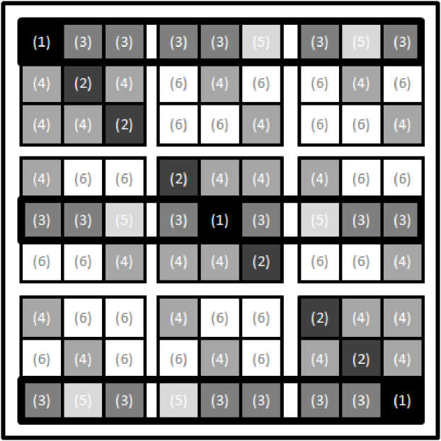
Figure 1: The pattern of $\mathbb{E}[W_{k}\otimes W_{k}]$ for $n=3$. The numbers in parentheses represent the value of each entry in terms of expressions $Q1$ to $Q6$ defined in (8). The entries that are different from the corresponding entries of $K\otimes K$ are marked with bold lines.

We now exploit the identified pattern to explicitly compute the left eigenvector $\mathbf{v}_{1}(\mathbb{E}[W_{k}\otimes W_{k}])$.

Lemma 1

The left eigenvector of $\mathbb{E}\left[W_{k}\otimes W_{k}\right]$ corresponding to its unit eigenvalue is given by

$$\mathbf{v}_{1}(\mathbb{E}[W_{k}\otimes W_{k}])=\frac{1}{\delta}\left[\rho(\mathbf{1}_{n}\mathbf{\otimes 1}_{n})+(1-\rho)\sum_{i=1}^{n}(\mathbf{e}_{i}\otimes\mathbf{e}_{i})\right]$$ (9)

where $\rho$ and $\delta$ depend on $p$ and $n$ as follows:

$$\rho(p,n) \triangleq \frac{p(n-1)}{p(n-2)+1-(1-p)^{n}},$$ (10)

$$\delta(p,n) \triangleq n+n(n-1)\rho(p,n).$$ (11)

Proof:

First of all, notice that $\mathbb{E}[W_{k}\otimes W_{k}]$ is a stochastic matrix whose entries are all strictly positive for $p>0$. Therefore, it has a unique left eigenvector corresponding to its unit eigenvalue, which means that $\mathbf{v}_{1}(\mathbb{E}[W_{k}\otimes W_{k}])$ is well-defined. We now show that the pattern of this left eigenvector is of the form

$$\mathbf{v}=\alpha(\mathbf{1}_{n}\mathbf{\otimes 1}_{n})+(\beta-\alpha)\sum_{i=1}^{n}(\mathbf{e}_{i}\otimes\mathbf{e}_{i}),$$ (12)

for some positive numbers $\alpha$ and $\beta$. Notice that all entries of this vector are equal to $\alpha$, except for the ones indexed $1+r(n+1)$ for $r=0,...,n-1$, which are equal to $\beta$. To show that the eigenvector we are looking for is indeed of the given pattern, we premultiply $\mathbb{E}[W_{k}\otimes W_{k}]$ by $\mathbf{v}$, and verify that

$$\mathbf{v}^{T}\mathbb{E}[W_{k}\otimes W_{k}]=\alpha^{\prime}(\mathbf{1\otimes 1})^{T}+(\beta^{\prime}-\alpha^{\prime})\sum_{i=1}^{n}(\mathbf{e}_{i}\otimes\mathbf{e}_{i})^{T}.$$ (13)

where $\alpha^{\prime}$ and $\beta^{\prime}$ are positive numbers, given by

$$\begin{bmatrix}\alpha^{\prime}\\ \beta^{\prime}\end{bmatrix}=\begin{bmatrix}A&B\\ C&D\end{bmatrix}\begin{bmatrix}\alpha\\ \beta\end{bmatrix}$$ (14)

with coefficients $A$, $B$, $C$, and $D$ defined as

$$A = 1+[nf_{1}(p,n)+n-2]\frac{1-f_{1}(p,n)}{(n-1)^{2}}$$

$$B = \frac{1-f_{1}(p,n)}{n-1}$$

$$C = [nf_{1}(p,n)+n-2]\frac{1-f_{1}(p,n)}{n-1}$$

$$D = f_{1}(p,n)$$

Equation (13) suggests that the pattern of $\mathbf{v}_{1}$ is preserved when it is multiplied by $\mathbb{E}[W_{k}\otimes W_{k}]$. Therefore, the vector defined in (12) is the unique left eigenvector of the matrix if there are positive numbers $\alpha=\alpha^{\prime}$ and $\beta=\beta^{\prime}$ that satisfy (14).

Due to the fact $BC=(1-A)(1-D)$, the matrix in (14) has an eigenvalue equal to one, with eigenvector $\begin{bmatrix}B&1-A\end{bmatrix}^{T}$, implying that such $(\alpha,\beta,\alpha^{\prime},\beta^{\prime})$ exist. Thus, the proposed vector in (12) is an eigenvector of $\mathbb{E}[W_{k}\otimes W_{k}]$ as long as $\alpha=\beta B/(1-A)=\rho(p,n)\beta$, which means that

$$\mathbf{v}_{1}(\mathbb{E}[W_{k}\otimes W_{k}])=\frac{1}{\delta}\left[\rho(\mathbf{1}_{n}\mathbf{\otimes 1}_{n})+(1-\rho)\sum_{i=1}^{n}(\mathbf{e}_{i}\otimes\mathbf{e}_{i})\right].$$

Note that $\delta(p,n)$, defined in (11), is a normalizing factor guaranteeing that the elements of the vector sum up to one. ∎

Now that we have derived explicit expressions for the eigenvectors (6) and (9), we can compute a closed-form expression for the variance of the limiting consensus value in terms of $p$ and $n$.

Theorem 2

The variance of the asymptotic consensus value $x^{\ast}$ of the distributed update defined in (1) over switching Erdős-Rényi random graphs with parameter $p$ is given by

$$\operatorname{var}(x^{\ast})=\frac{1-\rho}{\delta}\sum_{i=1}^{n}\left[x_{i}(0)-\bar{x}(0)\right]^{2},$$ (15)

where $\rho(p,n)$ and $\delta(p,n)$ are defined in (10) and (11), respectively.

Proof:

First, from (6), we have that

$$\left[\mathbf{x}(0)^{T}\mathbf{v}_{1}(\mathbb{E}W_{k})\right]^{2}=\left(\frac{1}{n}\sum_{i=1}^{n}x_{i}(0)\right)^{2}=\bar{x}(0)^{2}.$$

On the other hand, from (9), we have that

$$\left[\mathbf{x}(0)\otimes\mathbf{x}(0)\right]^{T}\mathbf{v}_{1}\left(\mathbb{E}[W_{k}\otimes W_{k}]\right)=$$

$$= \frac{1}{\delta}\left[\mathbf{x}(0)\otimes\mathbf{x}(0)\right]^{T}\left[\rho(\mathbf{1}_{n}\mathbf{\otimes 1}_{n})+(1-\rho)\sum_{i=1}^{n}(\mathbf{e}_{i}\otimes\mathbf{e}_{i})\right]$$

$$= \frac{\rho}{\delta}[\mathbf{x}(0)^{T}\mathbf{1}_{n}]\otimes[\mathbf{x}(0)^{T}\mathbf{1}_{n}]$$

$$+\frac{1-\rho}{\delta}\sum_{i=1}^{n}\left([\mathbf{x}(0)^{T}\mathbf{e}_{i}]\otimes[\mathbf{x}(0)^{T}\mathbf{e}_{i}]\right),$$

where we have used the fact that $(A\otimes B)(C\otimes D)=AC\otimes BD$. Since the Kronecker terms in the last expression are scalars, we have

$$[\mathbf{x}(0)\otimes\mathbf{x}(0)]^{T}\mathbf{v}_{1}(\mathbb{E}[W_{k}\otimes W_{k}])=\frac{\rho}{\delta}n^{2}\bar{x}(0)^{2}+\frac{1-\rho}{\delta}\sum_{i=1}^{n}x^{2}_{i}(0)$$

and therefore,

$$\operatorname{var}(x^{*})=\left(\frac{\rho}{\delta}n^{2}-1\right)[\bar{x}(0)]^{2}+\frac{1-\rho}{\delta}\sum_{i=1}^{n}[x_{i}(0)]^{2}.$$

By adding and subtracting $n\frac{1-\rho}{\delta}[\bar{x}\left(0\right)]^{2}$, the expression for the variance can be rewritten as

$$\operatorname{var}x^{*} = \frac{n(n-1)\rho+n-\delta}{\delta}[\bar{x}(0)]^{2}$$

$$+\frac{1-\rho}{\delta}\sum_{i=1}^{n}\left(x_{i}(0)-\bar{x}(0)\right)^{2}.$$

Since $\delta=n+n(n-1)\rho$, as defined in (11), the first term in the right-hand-side of the above expression is equal to zero. This proves the theorem. ∎

Expression (15) shows that, given the parameters of the random graph process $p$ and $n$, the variance of the limiting consensus value, $x^{\ast}$, is equal to the empirical variance of the initial conditions multiplied by the factor $n(1-\rho)/\delta$, which only depends on parameters $p$ and $n$.

IV Numerical Simulations

In this subsection, we present several simulations that illustrate the result in Theorem 2. In our first simulation, we compare the analytical expression for the variance in (15) with the empirical variance obtained from 100 realizations of the random consensus algorithm for $n$ in a certain range. In our simulations, we compute the (analytical and empirical) variances for a range of network sizes while keeping the expected out-degree of the random graphs fixed to a constant value $c$ (i.e., the probability communication in the random graphs is then $p=c/n$, for all $n$). In Fig. 1, we plot both the analytical and empirical variances when the network sizes $n$ goes from 5 to 50 nodes and the expected degree is fixed to be $c=5,$ for all $n$. The initial conditions for each network size is given by $x_{i}\left(0\right)=i/n$, for $i=1,...,n$.

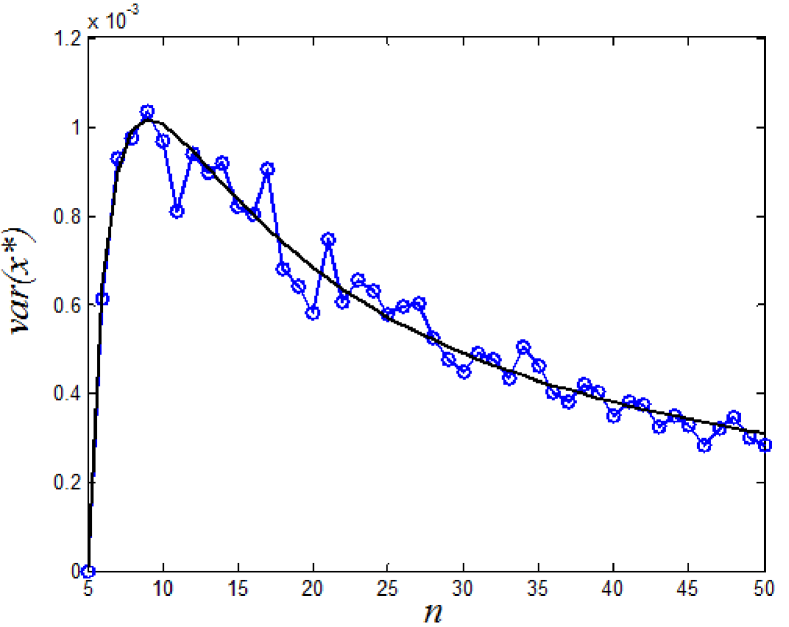
Figure 2: Comparison between the empirical variance and the analytical variance for $n$ in the interval [5:50] and $p=5/n$ for all $n$.

Several comments are in order about the behavior of $\operatorname{var}\left(x^{\ast}\right)$ in Fig. 1. First, for $n=c=5$, we have that $p=c/n=1$ (every link exist); hence, the random graph is not random, but a complete graph $K_{n}$, and the distributed consensus algorithm converges to the average of the initial conditions with zero variance (as one can check in Fig. 1). Second, when $n$ is slightly over $c$, the variance increases quite abruptly with $n$ until it reaches a maximum value. For $c=5$, this maximum is achieved for a network size of $9$ nodes. The location of this interesting point, that we denote by $\hat{n}\left(c\right)$, can be easily computed using Theorem 2. Furthermore, for $n>$ $\hat{n}(c)$ the variance slowly decreases with the network size. One can prove that this variance tends asymptotically to zero as $n\rightarrow\infty$ at a rate $1/n$.

Furthermore, according to (15), given a vector of $\mathbf{x}\left(0\right)$ initial condition, the variance of the asymptotic consensus value is equal to the empirical variance of the entries of $\mathbf{x}\left(0\right)$ rescaled by the factor $n\left(1-\rho\right)/\delta$ (where $\rho$ and $\delta$ depend on the random graph parameters $p$ and $n$). In Fig. 2, we plot the values of the factor $n\left(1-\rho\right)/\delta$ for a set of expected degrees $c\in\left\{5,6,7,8,9,10\right\}$ while the network size $n$ varies from $5$ to $70$. We observe that the behavior of the factor $n\left(1-\rho\right)/\delta$ is similar for any given $c$. Again, for $n=c$ the variances are zero and the variances grow abruptly until a maximum, $\hat{n}\left(c\right)$, is reached. For large values of $n$, the variance slowly decays towards zero at a rate $1/n$ for all $c$.

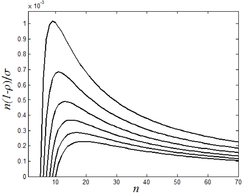
Figure 3: Several analytical variance for $c\in\left\{5,6,7,8,9,10\right\}$.

V Conclusions and Future Work

We have studied the asymptotic properties of the consensus value in distributed consensus algorithms over switching, directed random graphs. Due to the connectivity of the expected graph, consensus algorithms over Erdős-Rényi random graphs result in asymptotic agreement. However, the asymptotic value of consensus is not guaranteed to be the average of the initial conditions. Instead, agents will asymptotically agree on some random value in the convex hull of the initial conditions. While different aspects of consensus algorithms over random switching networks, such as conditions for convergence and the speed of convergence, have been widely studied, a characterization of the distribution of the asymptotic consensus for general asymmetric random consensus algorithms remains an open problem.

In this paper, we have derived closed-form expressions for the expectation and variance of the asymptotic consensus value as functions of the number of nodes $n$ and the probability of existence of a communication link, $p$. While the expectation of the distribution of the consensus value is simply the mean of the initial conditions over the nodes of the network, the variance presents an interesting structure. In particular, the variance of this limiting distribution of the consensus value is equal to the empirical variance of the set of initial conditions multiplied by a factor that depends on $p$ and $n$. We have derived an explicit expression for this factor and check its validity with numerical simulations.

[Kronecker Matrix Entries]

The Appendix contains the detailed computation of the entries of matrices $\mathbb{E}W_{k}$ and $\mathbb{E}[W_{k}\otimes W_{k}]$. We start by computing the elements of $\mathbb{E}W_{k}$. The diagonal entries of $\mathbb{E}W_{k}$ are given by:

$$\mathbb{E}w_{ii} = \mathbb{E}\left[\frac{1}{1+d_{i}}\right]=\sum_{k=0}^{n-1}\frac{1}{k+1}\mathbb{P}(d_{i}=k)$$

$$= \sum_{k=0}^{n-1}\frac{1}{k+1}\binom{n-1}{k}p^{k}(1-p)^{n-k-1}$$

$$= \frac{1-q^{n}}{np}\triangleq f_{1}(p,n)$$

On the other hand, the non-diagonal entries of $\mathbb{E}W_{k}$ result in:

$$\mathbb{E}w_{ij}=\frac{1}{n-1}[1-\mathbb{E}w_{ii}]=\frac{np-1+q^{n}}{np(n-1)}=\frac{1-f_{1}(p,n)}{n-1}$$

We now turn to the computation of the elements of $\mathbb{E}[W_{k}\otimes W_{k}]$, which are of the form $\mathbb{E}(w_{ij}w_{rs})$. In what follows we assume that the indices $i$, $j$, $r$, and $s$ are distinct. We first start with elements with in the diagonal subblocks of $\mathbb{E}[W_{k}\otimes W_{k}]$:

$$\mathbb{E}w_{ii}^{2} = \mathbb{E}\left[\frac{1}{(d_{i}+1)^{2}}\right]$$

$$= \sum_{k=0}^{n-1}\frac{1}{(k+1)^{2}}\binom{n-1}{k}p^{k}q^{n-k-1}$$

$$= q^{n-1}H(p,n)$$

For the rest of entries in the diagonal blocks, it is useful to note that $\mathbb{E}w_{ii}=f_{1}(p,n)$ and $\mathbb{E}w_{ij}=\frac{1-f_{1}(p,n)}{n-1}$, as proved in Subsection III-B:

$$\mathbb{E}(w_{ii}w_{rr}) = \mathbb{E}w_{ii}~{}\mathbb{E}w_{rr}=f_{1}^{2}(p,n)$$

$$\mathbb{E}(w_{ii}w_{ri}) = \mathbb{E}w_{ii}~{}\mathbb{E}w_{ri}=f_{1}(p,n)\frac{1-f_{1}(p,n)}{n-1}$$

$$\mathbb{E}(w_{ii}w_{rs}) = \mathbb{E}w_{ii}~{}\mathbb{E}w_{rs}=f_{1}(p,n)\frac{1-f_{1}(p,n)}{n-1}$$

$$\mathbb{E}(w_{ii}w_{is}) = \frac{\mathbb{E}w_{ii}-\mathbb{E}w_{ii}^{2}}{n-1}=\frac{f_{1}(p,n)-q^{n-1}H(p,n)}{n-1}$$

Similarly, we have the following results for the off-diagonal subblocks:

$$\mathbb{E}(w_{ij}w_{ji}) = \mathbb{E}w_{ij}~{}\mathbb{E}w_{ji}=\left(\frac{1-f_{1}(p,n)}{n-1}\right)^{2}$$

$$\mathbb{E}(w_{ij}w_{js}) = \mathbb{E}w_{ij}~{}\mathbb{E}w_{js}=\left(\frac{1-f_{1}(p,n)}{n-1}\right)^{2}$$

$$\mathbb{E}(w_{ij}w_{ri}) = \mathbb{E}w_{ij}~{}\mathbb{E}w_{ri}=\left(\frac{1-f_{1}(p,n)}{n-1}\right)^{2}$$

$$\mathbb{E}(w_{ij}w_{rj}) = \mathbb{E}w_{ij}~{}\mathbb{E}w_{rj}=\left(\frac{1-f_{1}(p,n)}{n-1}\right)^{2}$$

$$\mathbb{E}(w_{ij}w_{rs}) = \mathbb{E}w_{ij}~{}\mathbb{E}w_{rs}=\left(\frac{1-f_{1}(p,n)}{n-1}\right)^{2}$$

$$\mathbb{E}(w_{ij}w_{ii}) = \mathbb{E}(w_{ii}w_{is})=\frac{f_{1}(p,n)-q^{n-1}H(p,n)}{n-1}$$

$$\mathbb{E}(w_{ij}^{2}) = \mathbb{E}\left[\frac{a_{ij}^{2}}{(d_{i}+1)^{2}}\right]=\mathbb{E}\left[\frac{a_{ij}}{(d_{i}+1)^{2}}\right]$$

$$= \mathbb{E}(w_{ii}w_{ij})=\frac{f_{1}(p,n)-q^{n-1}H(p,n)}{n-1}$$

$$\mathbb{E}(w_{ij}w_{is}) = \frac{\mathbb{E}w_{ij}-\mathbb{E}w_{ij}^{2}-\mathbb{E}(w_{ij}w_{ii})}{n-2}$$

$$= \frac{1+2q^{n-1}H(p,n)-3f_{1}(p,n)}{(n-1)(n-2)}$$

References

- [1] J. N. Tsitsiklis, Problems in decentralized decision making and computation, Ph.D. dissertation, Massachusetts Institute of Technology, Cambridge, MA, 1984.
- [2] A. Jadbabaie, J. Lin, and A. S. Morse, “Coordination of groups of mobile autonomous agents using nearest neighbor rules,” IEEE Transactions on Automatic Control, vol. 48, no. 6, pp. 988-1001, 2003.
- [3] J. Cortes, S. Martinez, and F. Bullo, “Analysis and design tools for distributed motion coordination,” in Proceedings of the American Control Conference, Portland, OR, Jun. 2005, pp. 1680-1685.
- [4] M. H. DeGroot, “Reaching a Consensus,” Journal of American Statistical Association, vol. 69, no. 345, pp. 118-121, Mar. 1974.
- [5] B. Golub and M. O. Jackson, “Naive learning in social networks: Convergence, influence, and the wisdom of crowds,” 2007, unpublished Manuscript.
- [6] R. Olfati-Saber, J. A. Fax, and R. M. Murray, “Consensus and cooperation in networked multi-agent systems,” Proceedings of the IEEE, vol. 95, no. 1, Jan. 2007.
- [7] Y. Hatano and M. Mesbahi, “Agreement over random networks,” IEEE Transactions on Automatic Control, vol. 50, no. 11, pp. 1867-1872, 2005.
- [8] C. W. Wu, “Synchronization and convergence of linear dynamics in random directed networks,” IEEE Transactions on Automatic Control, vol. 51, no. 7, pp. 1207-1210, Jul. 2006.
- [9] M. Porfiri and D. J. Stilwell, “Consensus seeking over random weighted directed graphs,” IEEE Transactions on Automatic Control, vol. 52, no. 9, pp. 1767-1773, sep 2007.
- [10] A. Tahbaz-Salehi and A. Jadbabaie, “A necessary and sufficient condition for consensus over random networks,” IEEE Transactions on Automatic Control, vol. 53, no. 3, pp. 791-795, Apr 2008.
- [11] G. Picci and T. Taylor, “Almost sure convergence of random gossip algorithms,” in Proceedings of the 46th IEEE Conference on Decision and Control, New Orleans, LA, dec 2007, pp. 282-287.
- [12] D. Acemoglu, A. Ozdaglar, and A. ParandehGheibi, “Spread of (mis)information in social networks,” Massachusetts Institute of Technology, LIDS Report 2812, May 2009, submitted for Publication.
- [13] F. Fagnani and S. Zampieri, “Randomized consensus algorithms over large scale networks,” IEEE Journal on Selected Areas in Communications, vol. 26, no. 4, pp. 634-649, May 2008.
- [14] S. Boyd, A. Gosh, B. Prabhakar, and D. Shah, “Randomized gossip algorithms,” Special issue of IEEE Transactions on Information Theory and IEEE/ACM Transactions on Networking, vol. 52, no. 6, pp. 2508-2530, Jun. 2006.
- [15] A. Tahbaz-Salehi and A. Jadbabaie, “Consensus over ergodic stationary graph processes,” IEEE Transactions on Automatic Control, 2009, Accepted for Publication.