Conductance correlations in a mesoscopic spin glass wire :
a numerical Landauer study

Abstract

In this letter we study the coherent electronic transport through a metallic nanowire with magnetic impurities. The spins of these impurities are considered as frozen to mimic a low temperature spin glass phase. The transport properties of the wire are derived from a numerical Landauer technique which provides the conductance of the wire as a function of the disorder configuration. We show that the correlation of conductance between two spin configurations provides a measure of the correlation between these spin configurations. This correlation corresponds to the mean field overlap in the absence of any spatial order between the spin configurations. Moreover, we find that these conductance correlations are sensitive to the spatial order between the two spin configurations, i.e whether the spin flips between them occur in a compact region or not.

Spin glasses have been a focus of continuous interest in condensed matter for more than three decades. In spite of the relative simplicity of the models describing their physics, a precise understanding of their properties remains elusive. Spectacular progress has been made in understanding their nature at the mean field level Parisi (1980); Mézard et al. (1987), in characterizing their exotic aging properties in mean field models Cugliandolo (2002), including a proper description of the violation of the fluctuation-dissipation theorem, and experimentally in characterizing their memory and rejuvenation effects (see Vincent et al. (2009) for a recent review). However the applicability of mean field ideas in real samples remains debated Fisher and Huse (1986), with alternative approaches stressing the importance of the nature of excitations, and their consequences on various out-of-equilibrium properties of the phaseJ. Houdayer and Martin (2000).

A crucial quantity to characterize this spin glass physics is the correlation between different states of spins $\{\vec{S}_{i}^{(1)}\}_{i}$ and $\{\vec{S}_{i}^{(2)}\}_{i}$ in a given sample corresponding e.g to two different times $t_{1}$ and $t_{2}$ in a same quench, or two different quenches. For a single spin $i$, this correlation is naturally given by the local overlap $\vec{S}_{i}^{(1)}.\vec{S}_{i}^{(2)}$. For a collection of spins, mean-field theory neglects any spatial correlation of this local overlap : the correlation between the two spin states is given by

$$Q_{12}=\frac{1}{N}\sum_{i=1}^{N}\vec{S}_{i}^{(1)}.\vec{S}_{i}^{(2)}.$$ (1)

The distribution of this overlap between states reached after successive cooling in a sample plays a central role in the Parisi’s mean field theory. Note however that this overlap (1), while perfectly adequate at the mean field level, does not contain any information on the geometry of the correlation. In the simplest case of Ising spins it simply counts the number of spin flips between the two spin states, without any information on whether these spin flips occur in a compact region or randomly in the sample. Information about the spatial structure of this spin states correlation would require a more refined function.

Recently, building on previous theoretical work on sensitivity of conductance fluctuations to perturbations like magnetic impurities Al’tshuler and Spivak (1985) and pioneering experiments on conductance fluctuations in spin glasses de Vegvar et al. (1991); Jaroszynski et al. (1998); Neuttiens et al. (2000), the study of magneto-conductance of spin glass nanowires was proposed as a unique probe of these correlations between spin glass configurations Carpentier and Orignac (2008). Indeed, the correlation between conductances for two different mean-field like spin states depends monotonously on the overlap between these two states. Hence measurement of this conductance correlation can give access to the corresponding overlap Carpentier and Orignac (2008); Carpentier et al. (2009). This proposal calls for experimental and numerical studies of the correlations of conductance in a spin glass metallic system. It is the purpose of this letter to develop a numerical study of these conductance correlations, and in particular to address the question of sensitivity of these conductance correlations to spatial order between the corresponding spin states, originating from e.g the nature of excitation in the spin glass (see Cieplak et al. (1991) for an alternative numerical approach focused on the time evolution of conductance fluctuations). This question is naturally of crucial importance for experimental studies of quantum transport in spin glass nanowires. To address this question, we present a numerical Landauer approach allowing to accurately describe the weak localization regime of experimental relevance. This approach allows to go beyond the restrictions of analytical techniques and consider random spin states with spatial correlations between them.

To describe the electronic transport in the low temperature phase of a spin glass metallic wire, we consider a tight-binding Anderson model with magnetic disorder :

$$\mathcal{H}=\sum_{<i,j>,s}t_{ij}c_{j,s}^{\dagger}c_{i,s}+\sum_{i,s}v_{i}c_{i,s}^{\dagger}c_{i,s}\\ +J\sum_{i,s,s^{\prime}}{\vec{S}}_{i}.{\vec{\sigma}}_{s,s^{\prime}}c_{i,s}^{\dagger}c_{i,s^{\prime}},$$ (2)

where $t_{ij}=t$ represents the hopping of an electron from site $i$ to $j$, $v_{i}$ is the scalar random potential uniformly distributed in the interval $[-W/2;W/2]$ and $J$ is the intensity of the magnetic disorder which is typically smaller than $W$. The $\vec{\sigma}$ are Pauli matrices and $s$ labels the spin state of the electron. The magnetic impurities of the spin glass contribute to two different random potentials: a scalar diffusive potential $v_{i}$ (originating in part from the random positions of the impurities) and a magnetic disorder originating from the random spins ${\vec{S}}_{i}$. In this description, all impurity spins $\vec{S}_{i}$ are frozen and treated as classical spins. We choose the classical spins $\vec{S}_{i}$ randomly in the sphere of radius $S$, and independent from each other. This amounts to neglect any spatial order in a given state, in agreement with neutron scattering experiments Mydosh (1993). Going beyond this simple description by including more complex hidden spatial order goes beyond the scope of the present paper. Owing to the experimental findings of universal conductance fluctuations in the spin glass phasede Vegvar et al. (1991); Jaroszynski et al. (1998), we focus on the corresponding regime where the wire’s length $L_{x}$ is comparable or smaller than the inelastic dephasing length $L_{\phi}$, which effectively includes contribution from free spins. Without loss of generality, we will restrict ourselves to a two-dimensional ribbon of size (in units of lattice spacing) $L_{x}\times L_{y}$ with $L_{y}\ll L_{x}$.

For a given configuration of scalar disorder $V\equiv\{v_{i}\}_{i}$ and spins $\{{\vec{S}}_{i}\}_{i}$, we numerically determine the corresponding dimensionless conductance $g=G\times h/e^{2}$ through the Landauer formula Landauer (1957): $g=\sum_{n,m}\left|t_{nm}\right|^{2}$, where $n$ (resp. $m$) labels the propagating modes in the contacts and $t_{nm}$ the corresponding transmission amplitude. These transmission amplitudes are deduced from the electron’s retarded Green’s functions $G^{R}$ using the Fisher-Lee relation Fisher and Lee (1981). This Green’s function $G^{R}$ for the system connected to two semi-infinite leads is obtained by a recursive method MacKinnon (1980). The Fermi Energy is chosen so that the total number of transverse propagating modes is equal to $2\times L_{y}$. In units of $t=1$, the amplitude of scalar disorder is chosen as $W=0.6$ , while the coupling $J$ is varied from 0 (no magnetic disorder) to 0.4 (”strong” magnetic disorder). For fixed parameters, the conductance $g$ is a random function of both disorders $V$ and $\{{\vec{S}}_{i}\}_{i}$. We focus on the weak localization regime, where the conductance $g$ displays universal fluctuations of order $1$. Experimentally, these fluctuations are measured as a function of a weak transverse magnetic flux, assuming the ergodic hypothesis (see Tsyplyatyev et al. (2003) and Paulin and Carpentier (2009) for a numerical analysis). The amplitude of magneto-conductance fluctuations in a spin glass sample is given by the variance of the distribution of $g[V,\{{\vec{S}}_{i}\}_{i}]$ as $V$ is varied. In the rest of the article, for each configuration of spins the corresponding distribution will be sampled by $5000$ independent realizations of the scalar potential $V$.

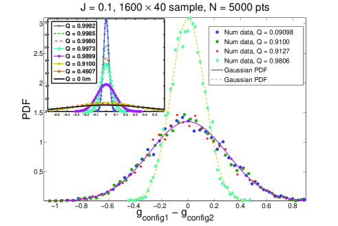
Figure 1: Probability Density Function of the difference $g[V,\{{\vec{S}}_{i}^{(1)}\}]-g[V,\{{\vec{S}}_{i}^{(2)}\}]$ as $V$ is varied. The result for various pairs of mean-field like spin states are shown, parametrized by the corresponding overlap between these spin states.

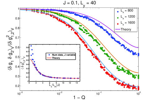
Figure 2: Conductance correlations as a function of spin configurations overlap for different longitudinal sizes, and normalized by their value for $Q_{12}=1$. In the inset, the conductance fluctuations ($Q_{12}=1$) are plotted as a function of $L_{x}/L_{m}$.

We start by identifying the regime of weak localization. In this regime, for a given random spin configuration, the variance of the above distribution of conductance $\langle(\delta g)^{2}\rangle=\langle\left(g[V,\{{\vec{S}}_{i}\}_{i}]-\langle g[V,\{{\vec{S}}_{i}\}_{i}]\rangle\right)^{2}\rangle$ (where $\langle\rangle$ corresponds to an average over $V$) is given in the 1D diffusive regime by

$$\langle(\delta g)^{2}\rangle=\frac{1}{4}F(0)+\frac{3}{4}F\left(\frac{2L_{x}}{\sqrt{3}L_{m}}\right)\\ +\frac{1}{4}F\left(\frac{2L_{x}}{L_{m}}\right)+\frac{1}{4}F\left(\frac{\sqrt{2}L_{x}}{\sqrt{3}L_{m}}\right)$$ (3)

where we defined Pascaud and Montambaux (1998) $F(x)=(6+6x^{2}-6\cosh(2x)+3x\sinh x)/(x^{4}\sinh^{2}x)$. The amplitude of these fluctuations extrapolate from $8/15$ for $L_{x}\ll L_{m}$ (orthogonal class with spin-degenerate states) to $1/15$ for $L_{x}\gg L_{m}$ (unitary class with double number of modes). The magnetic dephasing length $L_{m}$ depends in particular on the strength of magnetic disorder $J$. It is numerically determined through the use of formula (3). The inset of Fig. 2 shows the excellent agreement between the numerical data for this conductance fluctuations and weak localization formula (3) plotted as a function of $x=L_{x}/L_{m}(J)$.

Having determined the weak localization regime, we now turn to the study of correlations of the conductance between two different spin configurations $\{\vec{S}_{i}^{(1)}\}_{i}$ and $\{\vec{S}_{i}^{(2)}\}_{i}$. We consider the distribution as $V$ is varied of the difference $g\left[V,\{\vec{S}_{i}^{(1)}\}\right]-g\left[V,\{\vec{S}_{i}^{(2)}\}\right]$. This distribution has naturally zero mean, and its variance encodes statistical correlations between the two conductances $\left<(\delta g_{1}-\delta g_{2})^{2}\right>=2(\left<(\delta g_{1,2})^{2}\right>-\langle\delta g_{1}\delta g_{2}\rangle)$ where $g_{\alpha}=g\left[V,\{\vec{S}_{i}^{(\alpha)}\}\right]$. Similarly to the variance (3), they are parametrized by four dephasing lengths Al’tshuler and Spivak (1985); Carpentier and Orignac (2008); Fedorenko and Carpentier (2009) as follows

$$\langle\delta g_{1}\delta g_{2}\rangle=\frac{1}{4}F\left(L_{x}/L_{m}^{D,S}\right)+\frac{3}{4}F\left(L_{x}/L_{m}^{D,T}\right)\\ +\frac{1}{4}F\left(L_{x}/L_{m}^{C,S}\right)+\frac{3}{4}F\left(L_{x}/L_{m}^{C,T}\right)$$ (4)

with $F(y)$ given in (3) and the $L_{m}^{C/D,S/T}$ correspond to magnetic dephasing lengths for the Singlet/Triplet components of Diffuson/Cooperon contributions built between spin configurations $1$ and $2$. We will study these conductance correlations for different types of correlations between the spin configurations.

Mean-Field like excitations.

First, we consider spin states with no spatial correlations between them. These configurations are generated as follows : we start from a configuration $1$ where the orientations of spins are chosen randomly and independently from each other. From this first state, we generate other configurations by regenerating with a probability $p$ the orientations of each spin. In this case, the overlap (1) is an adequate measure of the correlation between these states. In practice with this method we generated spin states with mutual overlap $Q_{12}$ from $10^{-3}$ to $1$. For these spin configurations, we find a very good agreement with analytical studiesCarpentier and Orignac (2008) : the correlation between the conductances is entirely parametrized by their overlap $Q_{12}$. In Figure 1 we plot the probability density function (PDF) of the difference $g[V,\{{\vec{S}}_{i}^{(1)}\}]-g[V,\{{\vec{S}}_{i}^{(2)}\}]$ as $V$ is varied. The PDF for three different pairs of spin states with the same overlap $Q_{12}\simeq 0.91$ (dots, squares and triangles) are identical with each other and different from the PDF for a pair with $Q_{12}=0.98$. These PDF are found to be reasonably well Gaussian, parametrized solely by the above second cumulant.

Then we compare the behaviour of this second cumulant with eq.(4), using the analytical expressions to order $J^{2}$ for the dephasing lengths Carpentier and Orignac (2008) : $L_{m}^{D/C,S}=L_{m}/\sqrt{1\mp Q_{12}}$ and $L_{m}^{D/C,T}=L_{m}/\sqrt{1\pm Q_{12}/3}$. We find a reasonable agreement between this prediction and numerical results, as shown in Fig. 2. Note that this comparison is done without any free parameter as the magnetic dephasing length $L_{m}$ was determined from $\langle(\delta g)^{2}\rangle$ (see Fig. 3) The behaviour of this variance also explains the high sensitivity of $P(g_{1}-g_{2}\simeq 0)$ on small departures from $Q_{12}=1$ as shown in the inset of Fig. 1. Indeed, the probability of similar conductances reads $P(0)=1/\sqrt{2\pi\sigma}$ with $\sigma=2(\langle(\delta g)^{2}\rangle_{V}-\langle\delta g_{1}\delta g_{2}\rangle_{V})$.

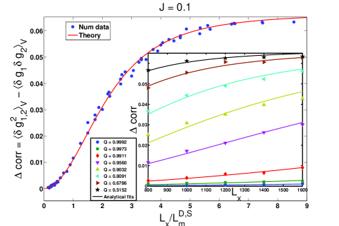
Figure 3: Comparison between the correlation between conductances $\sigma=2(\langle(\delta g)^{2}\rangle_{V}-\langle\delta g_{1}\delta g_{2}\rangle_{V})$ and the so-called Diffuson Singlet contribution $F(0)-F(L_{x}/L_{m}^{D,S})$. This contribution is found to be dominant in the region $Q_{12}\simeq 1$. In the inset we plot this $\sigma$ function for different value of overlap $Q_{12}$ and for $J=0.1$. Plain lines are theoretical fits allowing to determine $L_{m}^{D,S}(Q_{12},J)$. System size is $40\times 1600$.

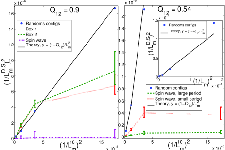
Figure 4: Left: evolution of the Diffuson Singlet dephasing rate of $1/(L_{m}^{D,S})^{2}$ as a function of the electronic dephasing rate $1/(L_{m}^{2})$ for mean-field like, spin wave (dash dot), and boxed excitations. The overlap is $0.9$ for all of them, and the size is $40\times 1600$. The linear dependance corresponds to the analytical expression $1/(L_{m}^{D,S})^{2}=(1-Q_{12})/(L_{m}^{2})$, valid in the absence of spatial correlations between the spin states. These results show the clear departure from this behavior for strong spatial correlations, and the absence of any effective overlap. Right: same evolution for random configurations and for spin wave with two different spatial periods corresponding to the same overlap ($Q=0.54$). The stronger correlation (longer period) corresponds to the larger deviation from the linear law.

From the above analytical expressions for $L_{m}^{C/D,S/T}$ for overlaps $Q_{12}\simeq 1$ the only diverging magnetic length is found to be $L_{m}^{D,S}$. Thus in this regime the expression (4) is dominated by the corresponding contribution Fedorenko and Carpentier (2009). This allows for a direct determination of $L_{m}^{D,S}$ from the $L_{x}-$dependance of $\sigma$ in the region $Q_{12}\simeq 1$, as shown in Fig. 3. We find an excellent agreement between the corresponding dephasing rate $1/(L_{m}^{D,S})^{2}$ and its perturbative analytical expression $(1-Q_{12})/(L_{m})^{2}$ as shown on Fig. 4.

Correlated excitations.

We now consider the influence of spatial correlation between two spin configurations. Generation of correlated spin configurations is obtained as follows: from an initial spin configuration we generate a configuration $n$ by reversing spins preferably inside a box of size $L_{x}^{(n)}\times L_{y}$ in the middle of the sample. We consider boxes of increases length $L_{x}^{(n)}=nL_{x}^{(1)}$, such that all states have the same overlap $Q$ with the initial configuration, but their spatial correlations with this initial configuration decreases with $n$ (the larger the box, the smaller the probability that a given spin inside the box is modified). We also generated spin wave like excitations: from the same initial spin configuration, each spin is rotated by $\delta\phi(x,y)=x\delta\phi_{0}$ around the $z-$axis (axis perpendicular to the planar sample). $\delta\phi_{0}$ determines the period of the spin wave, and thus the overlap between both configurations. For the different pairs of correlated spin configurations, we repeat the previous analysis of conductance correlations. In particular, we determine the Diffuson Singlet length $L_{m}^{D,S}$ for different values of magnetic disorder amplitude $J$ in the region $Q_{12}\simeq 1$. The result is shown in the left part of Fig. 4 for the overlap $Q_{12}=0.9$. We find clear deviation from the behavior $1/(L_{m}^{D,S})^{2}=(1-Q_{12})/(L_{m})^{2}$ which is valid in the absence of spatial correlations (Fig. 3). The deviation from this linear behavior is largest for the strongest spatial correlations between spin states, i.e for the smallest box excitations ($n=1$) and the spin wave excitations. We also consider two spin wave excitations with different period but the same overlap with an initial spin state (Fig. 4). Here again, the resulting Diffuson Singlet magnetic length is smaller for the strongest spatial correlation between the two spin states, corresponding to the largest period. These results demonstrate the sensitivity of the magnetic dephasing length $L_{m}^{D,S}$ on spatial correlations between the magnetic disorder configurations, and thus the influence of the geometry of random spin excitations on the associated correlation of conductances. Note that these results of Fig. 4 can in principle be tested experimentally by varying the density of magnetic impurities while working at fixed $T/T_{SG}$, allowing for an unprecedented test of e.g the nature of excitations in a spin glass state.

In this letter we presented a numerical Landauer analysis of transport in a mesoscopic metallic wire in the presence of frozen magnetic impurities. We have found that statistical properties of conductance correlations between two mean-field like spin configurations depend only on the corresponding spin overlap, in agreement with theoretical analysis. These results open the route to direct spin state correlations in mesoscopic spin glasses. We have also shown the crucial importance of spatial correlations between spin configurations in the electronic dephasing process. Studying these correlations along the lines of Fig. 4 could be experimentally achieved by varying the electronic density in diluted magnetic semiconductors. Unfortunately this would also modify the couplings between the impurity spins, and hence the spin configuration. A more promising route consists in exploring other multi-terminal geometries along the lines of de Vegvar et al. (1991).
We thank T. Capron for a much informative discussion concerning possible experimental test of our results. This work was supported by the ANR grants QuSpins and Mesoglass. All numerical calculations were performed on the computing facilities of the ENS-Lyon calculation center (PSMN).

References

- Parisi (1980) G. Parisi, J. Phys. A 13, 1101 (1980).
- Mézard et al. (1987) M. Mézard, G. Parisi, and M. Virasoro, Spin Glass Theory and Beyond (World Scientific, 1987).
- Cugliandolo (2002) L. Cugliandolo, in Lecture notes, Les Houches (2002).
- Vincent et al. (2009) E. Vincent, J. Hamman, and M. Ocio, in Wandering with Curiosity in Complex Landscapes, edited by J. of Statistical Physics (2009), vol. to appear.
- Fisher and Huse (1986) D. Fisher and D. Huse, Phys. Rev. Lett. 56, 1601 (1986).
- J. Houdayer and Martin (2000) F. K. J. Houdayer and O. C. Martin, Eur. Phys. J. B 18, 467 (2000).
- Al’tshuler and Spivak (1985) B. Al’tshuler and B. Spivak, JETP Lett. 42, 447 (1985).
- de Vegvar et al. (1991) P. de Vegvar, L. Lévy, and T. Fulton, Phys. Rev. Lett. 66, 2380 (1991).
- Jaroszynski et al. (1998) J. Jaroszynski, J. Wrobel, G. Karczewski, T. Wojtowicz, and T. Dietl, Phys. Rev. Lett. 80, 5635 (1998).
- Neuttiens et al. (2000) G. Neuttiens, C. Strunk, C. V. Haesendonck, and Y. Bruynseraede, Phys. Rev. B 62, 3905 (2000).
- Carpentier and Orignac (2008) D. Carpentier and E. Orignac, Phys. Rev. Lett. 100, 057207 (2008).
- Carpentier et al. (2009) D. Carpentier, E. Orignac, G. Paulin, and T. Roscilde, Int. J. of Nanotechnology to appear (2009).
- Cieplak et al. (1991) M. Cieplak, B. Bulka, and T. Dietl, Phys. Rev. B 44, 12337 (1991).
- Mydosh (1993) J. Mydosh, Spin Glasses, An Experimental Introduction (Taylor and Francis, London, 1993).
- Landauer (1957) R. Landauer, IBM J. Res. Dev. 1, 223 (1957).
- Fisher and Lee (1981) D. S. Fisher and P. Lee, Phys. Rev. B 23, 6851 (1981).
- MacKinnon (1980) A. MacKinnon, J. Phys. C 13, L1031 (1980).
- Tsyplyatyev et al. (2003) O. Tsyplyatyev, I. Aleiner, V. Fal’ko, and I. Lerner, Phys. Rev. B 68, 121301 (2003).
- Paulin and Carpentier (2009) G. Paulin and D. Carpentier (2009), preprint.
- Pascaud and Montambaux (1998) M. Pascaud and G. Montambaux, Physics - Uspekhi 41, 182 (1998).
- Fedorenko and Carpentier (2009) A. A. Fedorenko and D. Carpentier (2009), arXiv:0904.1011.