Instanton effects on Wilson–loop correlators: a new comparison with numerical results from the lattice

Abstract

Instanton effects on the Euclidean correlation function of two Wilson loops at an angle $\theta$, relevant to soft high–energy dipole–dipole scattering, are calculated in the Instanton Liquid Model and compared with the existing lattice data. Moreover, the instanton–induced dipole–dipole potential is obtained from the same correlation function at $\theta=0$, and compared with preliminary lattice data.

IFUP–TH/2009–17          

          Revised version          
April 2010          

1 Introduction

Since its discovery in 1975 [1], the instanton solution of the Yang–Mills equations has been widely studied, both in its mathematical properties and its phenomenological applications [2, 3, 4, 5, 6, 7, 8]. Many insights have been obtained in QCD through the use of instantons (see, e.g., the review [9] and references therein), and even if it is known that they cannot provide the framework for a complete understanding of strong interactions, it is interesting to investigate instanton effects as they contribute to the nonperturbative dynamics.

Among the various open problems in QCD, soft high–energy hadron–hadron scattering is known to be of nonperturbative nature, and so it is worth studying what the consequences are of instantons on the scattering amplitudes. In the approach from the first principles of QCD [10], such amplitudes are related to properties of the vacuum, namely the correlation functions of certain Wilson–line and Wilson–loop operators. In particular, in the case of meson–meson scattering, the scattering amplitudes can be reconstructed, after folding with the appropriate mesonic wave functions, from the scattering amplitude of two colour dipoles of fixed transverse size; the latter are obtained from the correlation function of two rectangular Wilson loops, describing (in the considered energy regime) the propagation of the colour dipoles [11, 12, 13, 14, 15]. The physical, Minkowskian correlation functions can be reconstructed from the “corresponding” Euclidean correlation functions [16, 17, 18, 19, 20, 21, 22], and so it has then been possible to investigate the problem of soft high–energy scattering with some nonperturbative techniques available in Euclidean Quantum Field Theory [23, 24, 25, 26, 27, 28].

In this paper we shall derive a quantitative prediction of instanton effects in the Euclidean loop–loop correlation function, relevant to the problem of soft high–energy scattering. This problem has already been addressed in Ref. [23], using the so–called Instanton Liquid Model (ILM) [8], but the result reported in that paper contains a severe divergence, apparently not noticed by the authors. In this paper we critically repeat the calculation, obtaining a well–defined analytic expression, which can be compared with the lattice data presented and discussed in Ref. [28]. In this paper we also calculate the instanton–induced dipole–dipole potential from the correlation function of two parallel Wilson loops [29], and we compare the results with some preliminary data from the lattice.

The detailed plan of this paper is the following. In Section 2 we briefly recall the main features of instantons in Yang–Mills theory, we shortly describe the relevant aspects of the ILM, and we discuss the method we will actually use in our calculations, using as an example the expectation value of a rectangular Wilson loop and the instanton–induced $q\bar{q}$–potential [6, 30]. In Section 3, after a brief review of how high–energy scattering amplitudes can be reconstructed from the correlation function of two rectangular Wilson loops at an angle $\theta$ in Euclidean space, we evaluate this same correlation function and we critically compare the result with the calculation of Ref. [23]. We then compare our quantitative prediction with the lattice results of Ref. [28]. In Section 4 we calculate the correlation function of two parallel Wilson loops, from which we derive the instanton–induced dipole–dipole potential, that we compare with some preliminary data from the lattice. Finally, in Section 5 we draw our conclusions. Some technical details are discussed in the Appendices.

2 Wilson loops in the ILM

Instantons (anti–instantons) are self–dual (anti–self–dual) solutions with finite action of the classical Yang–Mills equations of motion in Euclidean space [1]. We will be interested only in the solutions with topological charge $q=+1$ and $q=-1$, which we will refer to as the instanton (${\rm I}$) and the anti–instanton ($\bar{\rm I}$), respectively. In the case of $SU(2)$ Yang–Mills theory, the instanton solution in regular covariant (Lorenz) gauge reads, for the standard colour orientation,

$$A_{\mu}^{a}(x;z,{\rm I})=-\frac{2}{g}\frac{\eta_{a\mu\nu}(x-z)_{\nu}}{(x-z)^{2}+\rho^{2}},\qquad A_{\mu}=A_{\mu}^{a}\frac{\sigma^{a}}{2},\,\,a=1,2,3,$$ (2.1)

where $z_{\mu}$ and $\rho$ are free parameters that correspond to the position of the center and the radius of the instanton, respectively, $\eta_{a\mu\nu}$ are the self–dual ’t Hooft symbols [5], and $\sigma^{a}$ are the Pauli matrices. The anti–instanton solution $A_{\mu}^{a}(x;z,\bar{\rm I})$ is obtained by replacing $\eta_{a\mu\nu}\to\bar{\eta}_{a\mu\nu}$ in Eq. (2.1), where the latter are the anti–self–dual ’t Hooft symbols [5]. Applying a $SU(2)$ transformation on Eq. (2.1), $A_{\mu}\to UA_{\mu}U^{\dagger}$ with $U\in SU(2)$, we obtain another solution with a different colour orientation. Instantons in $SU(N_{c})$ Yang–Mills theory can be obtained by embedding the $SU(2)$ solution (2.1) in a $SU(2)$ subgroup of $SU(N_{c})$, and it has been shown that these are the only solutions with $|q|=1$ [7]. We will take the standard–oriented solution to be the embedding of the (standard) $SU(2)$ solution in the upper–left $2\times 2$ corner of an $N_{c}\times N_{c}$ matrix; the other solutions are obtained by applying an $SU(N_{c})$ colour rotation on this one.

Early attempts at a description of the QCD vacuum in terms of an ensemble of instantons and anti–instantons adopted the picture of a dilute gas [6], but suffered from severe infrared divergences due to the presence of large–size instantons. The proposal of [8] was instead that the pseudoparticles form a dilute liquid: the diluteness of the medium allows for a meaningful description in terms of individual pseudoparticles, while the infrared problem is solved assuming that interactions stabilise the instanton radius. In particular, this model assumes that the vacuum can be described as a liquid of instantons and anti–instantons, with equal densities $n_{{\rm I}}=n_{\bar{\rm I}}=n/2$, and with radius distributions strongly peaked around the same average value: in practice, one performs the calculations using a $\delta$–like distribution, i.e., fixing the radii of the pseudoparticles to a given value $\rho$. Using the SVZ sum rules [31, 32] to relate vacuum properties with experimental quantities, the phenomenological values for the total density and the average radius are estimated to be [9] $n\simeq 1{\rm\,fm}^{-4}$, $\rho\simeq 1/3{\rm\,fm}$, which lead to a small packing fraction $nV_{1}\sim 1/20$ [here $V_{1}=(\pi^{2}/2)\rho^{4}$ is the volume of a 3–sphere of radius $\rho$, which is approximately the space–time volume occupied by a single pseudoparticle]; this indicates that the instanton liquid is indeed fairly dilute. We refer the interested reader to [9] and references therein for a more detailed discussion of the model, both on its theoretical foundations [33, 34] and on the development of numerical methods of investigation [35]. In the rest of this paper we will make use only of the general picture described above to give estimates of the relevant quantities.

To calculate the expectation value of an operator $\cal O$ one needs to average over the ensemble with some density function ${\cal D}={\cal D}(\{z\},\{U\})$, where $\{z\}$ denotes collectively the coordinates of the pseudoparticles and $\{U\}$ their orientations in colour space; in principle, such a function should be determined by properly taking instanton interactions into account. Starting with an ensemble of $N_{{\rm I}}$ instantons and $N_{\bar{\rm I}}$ anti–instantons in a space–time volume $V$, we obtain the desired result by taking the “thermodynamic limit” $N_{{\rm I}},N_{\bar{\rm I}},V\to\infty$, while keeping the densities $n_{{\rm I}}\equiv N_{{\rm I}}/V$ and $n_{\bar{\rm I}}\equiv N_{\bar{\rm I}}/V$ fixed:

$$\langle{\cal O}\rangle_{\rm ILM}\equiv\lim_{\begin{subarray}{c}N_{{\rm I},\bar{\rm I}},V\to\infty,\\ n_{{\rm I},\bar{\rm I}}\,{\rm f\mbox{}ixed}\end{subarray}}{\displaystyle\int d^{4N}z\,d^{N}U\,{\cal D}(\{z\},\{U\})\,{\cal O}(\{z\},\{U\})}.$$ (2.2)

Here ${\cal O}(\{z\},\{U\})$ denotes the operator $\cal O$ evaluated in the field configuration generated by the pseudoparticles, and $dU$ is the normalised Haar measure, $\int dU=1$. Since the medium is dilute, the field configuration is approximately equal to the superposition of single (anti–)instanton fields,

$$A_{\mu}(x)=\sum_{i=1}^{N}U(i)A_{\mu}(x;z_{i},\sigma_{i})U^{\dagger}(i),$$ (2.3)

where $N=N_{{\rm I}}+N_{\bar{\rm I}}$ is the total pseudoparticle number, $z_{i}$ and $U(i)$ are the position and colour orientation of pseudoparticle $i$, respectively, and $\sigma_{i}={\rm I},\bar{\rm I}$ indicates if pseudoparticle $i$ is an instanton or an anti–instanton.

To perform calculations, we take an approximate density function that describes the instanton liquid as an ensemble of free particles with some (unspecified) strong core repulsion, which approximately localises the instantons in distinct “cells” of volume $V_{\rm cell}$, i.e.,

$${\cal D}(\{z\})={\cal N}^{-1}\sum_{P}\prod_{j=1}^{N}\chi_{D_{j}}(z_{P(j)}),\qquad{\cal N}=N!\,V_{\rm cell}^{N}$$ (2.4)

where $\{D_{j}\}$ is a partition in cells of the space–time region $D$ occupied by the ensemble, $\cup_{j}D_{j}=D$, $\chi_{D_{j}}$ is the characteristic function of $D_{j}$, $P$ denotes a permutation of $\{1,\ldots,N\}$, and ${\cal N}$ is the normalisation; the volume of each cell is $\int d^{4}z\,\chi_{D_{j}}(z)=V_{\rm cell}$. The coordinates of pseudoparticle $j$ are denoted as $z_{j}$, and we take the first $N_{{\rm I}}$ pseudoparticles to be instantons, and the remaining $N_{\bar{\rm I}}$ to be anti–instantons,

$$\sigma_{k}=\left\{\begin{aligned} &{\rm I},&&1\leq k\leq N_{{\rm I}},\\ &\bar{\rm I},&&N_{{\rm I}}+1\leq k\leq N.\end{aligned}\right.$$ (2.5)

The function (2.4) is by no means a precise description of the instanton ensemble: it has the purpose of capturing the main features of the liquid picture, namely the diluteness and the uniform density of the medium, while at the same time keeping the calculation feasible. Notice that ${\cal D}$ does not depend on the colour orientation of the pseudoparticles. The precise shape of the cells should not be important, and one can choose it according to the geometry of the problem.

For a local operator ${\cal O}_{\rm local}(x)$, only configurations with a single pseudoparticle located near the point $x$ have both non–negligible effects and non–negligible measure in configuration space, due to the diluteness of the medium and to the short–range nature of instanton effects. The evaluation of expectation values is more complicated for non–local operators such as Wilson lines and Wilson loops, since they involve the value of the fields on a curve ${\cal C}$. However, by properly subdividing ${\cal C}$ into small segments, one can exploit again the diluteness of the medium and the short–range nature of instanton effects, in order to consider each segment to be affected only by the field of a single pseudoparticle.

As an example, consider the case of the expectation value of a rectangular Wilson loop ${\cal W}$ of temporal extension $T$ and spatial width $R$ (say, in the $1$ direction). As it is well known, one can extract from this expectation value the static quark–antiquark potential ${\cal V}_{q\bar{q}}$ using the relation [36, 37]

$$\langle{\cal W}\rangle=\frac{1}{N_{c}}{\rm Tr}\,[{\rm W}^{(-){\dagger}}{\rm W}^{(+)}]\mathop{=}_{T\to\infty}{\cal K}e^{-T{\cal V}_{q\bar{q}}(R)},$$ (2.6)

where we have neglected the effect of the transverse “links” connecting the Wilson lines ${\rm W}^{(\pm)}$, which describe the propagation of the quark and of the antiquark, and where ${\cal K}$ is some proportionality constant. The effect of a single instanton located at $z$ on an infinite Wilson loop, which we denote with $w(z,{\rm I})$, is given by the following expression [6],

$$w(z,{\rm I})\equiv 1-\frac{2}{N_{c}}\Delta(z),$$ (2.7)

where

$$\Delta(z)=1-\cos\alpha_{+}\cos\alpha_{-}-\hat{n}_{+}\cdot\hat{n}_{-}\sin\alpha_{+}\sin\alpha_{-}\,,$$ (2.8)

$$\alpha_{\pm}=\frac{\pi\|n_{\pm}\|}{\sqrt{\|n_{\pm}\|^{2}+\rho^{2}}}\,,\qquad n^{a}_{\pm}=-(\pm\frac{R}{2}\delta_{1a}-z_{a})\,.$$

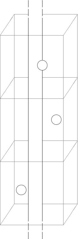
Figure 1: Schematic representation of a Wilson loop in the instanton liquid. Circles represent pseudoparticles with the same radius $\rho$, each lying in a cell.

The result does not depend on the colour orientation of the instanton, and it does not change if we replace the instanton with an anti–instanton. In order to calculate the effect of the instanton liquid, i.e., of the whole ensemble, on the Wilson loop, it is natural to see it as the result of a time series of interactions between the colour dipole and the pseudoparticles: this suggests dividing space–time into time–slices of thickness $\delta T$, and then each slice into cells of volume $V_{\rm cell}=V_{\rm cell}^{(3)}\,\delta T$. The situation is illustrated in Fig. 1. Here $\delta T$ and $V_{\rm cell}^{(3)}$ are determined by the following requirements:

1. only one pseudoparticle falls in $V_{\rm cell}^{(3)}\,\delta T$ on the average, i.e., $nV_{\rm cell}=1$;

2. the spatial size $V_{\rm cell}^{(3)}$ is large enough to accommodate the whole dipole, and also large enough so that the pseudoparticles which fall outside of the cell where the dipole lies will not affect it, being too distant;

3. $\delta T$ is large enough for an (anti–)instanton to fully affect the portions of the two Wilson lines that fall in $V_{\rm cell}$, i.e., $\delta T$ can be considered infinite ($\delta T\gg\rho$) as far as the colour rotation induced on the Wilson lines by the pseudoparticle is concerned, and so one can use the colour rotation angles $\alpha_{\pm}$ given in Eq. (2.8).

The region of 3–space where an (anti–)instanton can affect the operator is approximately determined by requiring that the pseudoparticle is not too far from the two long sides (say, more than $\rho$), which implies

$$V_{\rm cell}^{(3)}\sim(R+2\rho)(2\rho)^{2};$$ (2.9)

in this way the two segments of the loop lying in a given slice fall in the same cell. With this choice we fulfill condition (2.); imposing condition (1.) we obtain

$$\frac{\delta T}{\rho}\sim\frac{81\rho}{4(R+2\rho)}\sim\frac{10}{1+\frac{R}{2\rho}},$$ (2.10)

which is reliable for $R\lesssim 2\rho$, so that $\delta T/\rho\gtrsim 5$ in this regime, and condition (3.) is satisfied. For larger dipoles, the quark and the antiquark are more likely to interact with distinct instantons: the expectation value should then factorise for large $R$.

At this point one can perform the average over the instanton ensemble: since the procedure is the same as the one adopted in [6], we will not report the calculation here, and we simply quote the result which will be used in the following:

$$\langle{\cal W}\rangle_{\rm ILM}=e^{-T{\cal V}_{q\bar{q}}(R)},\quad{\cal V}_{q\bar{q}}(R)=n\frac{2}{N_{c}}\int d^{3}z\,\Delta(z).$$ (2.11)

This result is the same as the one found in Ref. [30] with different, more sophisticated methods. As $\Delta(z)$ is localised around the position in 3–space of the quark and the antiquark, for large $R$ the Wilson–loop expectation value factorises, and the potential becomes the sum of two constant and equal terms, which are interpreted as the renormalisation of the quark mass [30].

3 High–energy meson–meson scattering and the Wilson–loop correlation functions in the ILM

As has already been recalled in the Introduction, in the soft high–energy regime the mesonic scattering amplitudes can be reconstructed from the correlation function of two Euclidean Wilson loops. In this Section we give first a brief account, for the benefit of the reader, of the main points of the functional–integral approach to the problem of elastic meson–meson scattering, referring the interested reader to the original papers [11, 12, 13, 14, 15] and to the book [38]. We shall use the same notation adopted in Ref. [28], where a more detailed presentation can be found. We then critically repeat the calculation of the relevant correlation function in the ILM, and compare the result with the one found in Ref. [23].

The elastic scattering amplitudes of two mesons (taken for simplicity with the same mass $m$) in the soft high–energy regime can be reconstructed in two steps. One first evaluates the scattering amplitude of two $q\bar{q}$ colour dipoles of fixed transverse sizes $\vec{R}_{1\perp}$ and $\vec{R}_{2\perp}$, and fixed longitudinal momentum fractions $f_{1}$ and $f_{2}$ of the two quarks in the two dipoles, respectively; the mesonic amplitudes are then obtained after folding the dipoles’ amplitudes with the appropriate squared wave functions, describing the interacting mesons. The dipole–dipole amplitudes are given by the 2–dimensional Fourier transform, with respect to the transverse distance $\vec{z}_{\perp}$, of the normalised (connected) correlation function of two rectangular Wilson loops,

$${\cal M}_{(dd)}(s,t;\vec{R}_{1\perp},f_{1},\vec{R}_{2\perp},f_{2})\equiv-i~{}2s\displaystyle\int d^{2}\vec{z}_{\perp}e^{i\vec{q}_{\perp}\cdot\vec{z}_{\perp}}{\cal C}_{M}(\chi;\vec{z}_{\perp};1,2),$$ (3.1)

where the arguments “$1$” and “$2$” stand for “$\vec{R}_{1\perp},f_{1}$” and “$\vec{R}_{2\perp},f_{2}$” respectively, $t=-|\vec{q}_{\perp}|^{2}$ ($\vec{q}_{\perp}$ being the transferred momentum) and $s=2m^{2}(1+\cosh\chi)$. The correlation function ${\cal C}_{M}$ is defined as the limit $\displaystyle{\cal C}_{M}\equiv\lim_{T\to\infty}{\cal G}_{M}$ of the correlation function of two loops of finite length $2T$,

$${\cal G}_{M}(\chi;T;\vec{z}_{\perp};1,2)\equiv\dfrac{\langle{\cal W}^{(T)}_{1}{\cal W}^{(T)}_{2}\rangle_{M}}{\langle{\cal W}^{(T)}_{1}\rangle_{M}\langle{\cal W}^{(T)}_{2}\rangle_{M}}-1,$$ (3.2)

where $\langle\ldots\rangle_{M}$ are averages in the sense of the QCD (Minkowskian) functional integral. Here ${\cal W}^{(T)}_{1,2}$ are Minkowskian Wilson loops evaluated along the paths ${\cal C}_{1,2}$, made up of the classical trajectories of the quarks and antiquarks inside the two mesons, and closed by straight–line paths in the transverse plane at proper times $\pm T$. The partons’ trajectories form a hyperbolic angle $\chi$ in the longitudinal plane, and they are located at $(1-f_{i})\vec{R}_{i\perp}$ (quark) and $-f_{i}\vec{R}_{i\perp}$ (antiquark), $i=1,2$, in the transverse plane.

The Euclidean counterpart of Eq. (3.2) is

$${\cal G}_{E}(\theta;T;\vec{z}_{\perp};1,2)\equiv\dfrac{\langle{\cal W}^{(T)}_{1}{\cal W}^{(T)}_{2}\rangle_{E}}{\langle{\cal W}^{(T)}_{1}\rangle_{E}\langle{\cal W}^{(T)}_{2}\rangle_{E}}-1,$$ (3.3)

where now $\langle\ldots\rangle_{E}$ is the average in the sense of the Euclidean QCD functional integral. With a little abuse of notation, we denote with the same symbol ${\cal W}^{(T)}_{1,2}$ the Euclidean Wilson loops calculated on the following straight–line paths,

$${\cal C}_{1}: \quad X^{1q}_{\mu}(\tau)=z_{\mu}+u_{1\mu}\tau+(1-f_{1})R_{1\mu},~{}~{}~{}~{}X^{1\bar{q}}_{\mu}(\tau)=z_{\mu}+u_{1\mu}\tau-f_{1}R_{1\mu},$$

$${\cal C}_{2}: \quad X^{2q}_{\mu}(\tau)=u_{2\mu}\tau+(1-f_{2})R_{2\mu},~{}~{}~{}~{}X^{2\bar{q}}_{\mu}(\tau)=u_{2\mu}\tau-f_{2}R_{2\mu},$$ (3.4)

with $\tau\in[-T,T]$, and closed by straight–line paths in the transverse plane at $\tau=\pm T$. Here

$$u_{1}=\left(\sin\frac{\theta}{2},\vec{0}_{\perp},\cos\frac{\theta}{2}\right),~{}~{}~{}u_{2}=\left(-\sin\frac{\theta}{2},\vec{0}_{\perp},\cos\frac{\theta}{2}\right),$$ (3.5)

and $R_{1}=(0,\vec{R}_{1\perp},0)$, $R_{2}=(0,\vec{R}_{2\perp},0)$, $z=(0,\vec{z}_{\perp},0)$. Again, we define the correlation function with the IR cutoff $T$ removed as $\displaystyle{\cal C}_{E}\equiv\lim_{T\to\infty}{\cal G}_{E}$.

It has been shown in [18, 19, 22] that the correlation functions in the two theories are connected by the analytic–continuation relations

$${\cal G}_{M}(\chi;T;\vec{z}_{\perp};1,2) = {\cal G}_{E}(-i\chi;iT;\vec{z}_{\perp};1,2),\qquad\forall\,\chi\in\mathbb{R}^{+},$$

$${\cal G}_{E}(\theta;T;\vec{z}_{\perp};1,2) = {\cal G}_{M}(i\theta;-iT;\vec{z}_{\perp};1,2),\qquad\forall\,\theta\in(0,\pi).$$ (3.6)

Under certain analyticity hypotheses in the $T$ variable, the following relations are obtained for the correlation functions with the IR cutoff $T$ removed [19, 22]:

$${\cal C}_{M}(\chi;\vec{z}_{\perp};1,2) = {\cal C}_{E}(-i\chi;\vec{z}_{\perp};1,2),\qquad\forall\,\chi\in\mathbb{R}^{+},$$

$${\cal C}_{E}(\theta;\vec{z}_{\perp};1,2) = {\cal C}_{M}(i\theta;\vec{z}_{\perp};1,2),\qquad\phantom{-}\forall\,\theta\in(0,\pi).$$ (3.7)

We turn now to the calculation of instanton effects on the correlation function ${\cal C}_{E}$. As it is explained in Appendix A, we can set $f_{1}=f_{2}=1/2$ without loss of generality; we also drop the dependence on $f_{i}$ in the following formulas, i.e., we understand ${\cal C}_{E}(\theta;\vec{z}_{\perp};\vec{R}_{1\perp},\vec{R}_{2\perp})\equiv{\cal C}_{E}(\theta;\vec{z}_{\perp};\vec{R}_{1\perp},f_{1}=1/2,\vec{R}_{2\perp},f_{2}=1/2)$. Neglecting the transverse links connecting the quark and antiquark trajectories, the Wilson loops are written as

$${\cal W}_{i}^{(T)}=\frac{1}{N_{c}}{\rm Tr}\,[{\rm W}^{(\bar{q}){\dagger}}_{i}{\rm W}^{(q)}_{i}],\qquad i=1,2,$$ (3.8)

with

$${\rm W}^{(\bar{q})}_{i} ={\cal P}\exp\left[-ig\displaystyle\int_{-T}^{T}A_{\mu}(X^{i\bar{q}}(\tau)){u_{i\mu}}d\tau\right],\qquad i=1,2$$ (3.9)

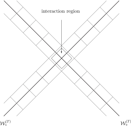
Figure 2: Longitudinal projection of the two loops, showing the partition in cells relevant to the case of loops at an angle $\theta$.

and similarly for ${\rm W}^{(q)}_{i}$. Since the (long) sides of the two loops have different directions in the longitudinal plane, their relative distance grows as we move away from the center of the configuration; as a consequence, only pseudoparticles falling in a finite interaction region have effects on both loops (see Fig. 2), and will therefore contribute to the connected part of the loop–loop correlator. This region is roughly determined by requiring that the distance of the pseudoparticles from both loops in the transverse and in the longitudinal plane does not exceed $\sim\rho$. Then $V_{\rm int}=V_{\parallel}V_{\perp}$, where $\parallel$ and $\perp$ refer to the longitudinal and transverse planes, respectively, with

$$V_{\perp} \sim\left(|\vec{z}_{\perp}|+\frac{|\vec{R}_{1\perp}|+|\vec{R}_{2\perp}|}{2}+2\rho\right)\left(\frac{|\vec{R}_{1\perp}|+|\vec{R}_{2\perp}|}{2}+2\rho\right),$$ (3.10)

$$V_{\parallel} \sim\frac{(2\rho)^{2}}{\sin\theta}.$$ (3.11)

We now make the following approximation, considering only one instanton or anti–instanton in the interaction region, all the other pseudoparticles interacting with one loop only (or not interacting at all with the loops). Clearly, $V_{\parallel}$ blows up as $\theta\to 0,\pi$, and so does the number of pseudoparticles in the interaction region $nV_{\rm int}\propto n\rho^{4}/\sin\theta$; thus, the one–instanton approximation can be good if the angle is not too close to $0,\pi$. In this case we can perform the integration over the colour degrees of freedom independently for the two loops, except for the pseudoparticle in the interaction region, but since this last integration is trivial we obtain simply

$${\cal W}_{1}^{(T)}{\cal W}_{2}^{(T)}\to\left[\prod{}^{{}^{\prime}}w_{1}(k)\prod{}^{{}^{\prime}}w_{2}(k)\right]w_{1}(0)w_{2}(0),$$ (3.12)

where the prime indicates that we exclude the terms corresponding to the interaction region, and $0$ refers to the interacting pseudoparticle. Here $w_{i}(k)=1-(2/N_{c})\Delta_{i}(x_{P(k)})$, with $x_{P(k)}$ being the position of the pseudoparticle lying in the $k$–th cell [see Eq. (2.7)], and with

$$\Delta_{i}(x) =1-\cos\alpha_{i+}\cos\alpha_{i-}-\hat{n}_{i+}\cdot\hat{n}_{i-}\sin\alpha_{i+}\sin\alpha_{i-},$$

$$\alpha_{i\pm} =\frac{\pi\|n_{i\pm}\|}{\sqrt{\|n_{i\pm}\|^{2}+\rho^{2}}},$$

$$n^{a}_{1\pm} =\eta_{a\mu\nu}u_{1\mu}(z\pm\frac{R_{1}}{2}-x)_{\nu},\quad n^{a}_{2\pm}=\eta_{a\mu\nu}u_{2\mu}(\pm\frac{R_{2}}{2}-x)_{\nu}.$$ (3.13)

Performing the integration over the pseudoparticle positions, making use of formula (B.7) in Appendix B, and dividing by the expectation values of the loops [see Eq. (2.11)] we finally obtain for the normalised connected correlation function with $T\to\infty$

$${\cal C}_{E}^{\rm(ILM)}(\theta;\vec{z}_{\perp};\vec{R}_{1\perp},\vec{R}_{2\perp})\\ =\dfrac{\displaystyle 1+n\int_{\rm int}d^{4}x\left[\left(1-\frac{2}{N_{c}}\Delta_{1}(x)\right)\left(1-\frac{2}{N_{c}}\Delta_{2}(x)\right)-1\right]}{\displaystyle\left[1-n\int_{\rm int}d^{4}x\,\frac{2}{N_{c}}\Delta_{1}(x)\right]\left[1-n\int_{\rm int}d^{4}x\,\frac{2}{N_{c}}\Delta_{2}(x)\right]}-1,$$ (3.14)

where “int” indicates that the integration range is restricted to the interaction region, since all the other terms cancel between the numerator and denominator. Expanding to first order in $n$, for consistency with the one–instanton approximation, we finally get

$${\cal C}_{E}^{\rm(ILM)}(\theta;\vec{z}_{\perp};\vec{R}_{1\perp},\vec{R}_{2\perp})=n\left(\frac{2}{N_{c}}\right)^{2}\int d^{4}x\,\Delta_{1}(x)\Delta_{2}(x),$$ (3.15)

having extended the integration range to the whole space–time since the integrand is now rapidly vanishing. Exploiting the properties of the ’t Hooft symbols we find

$$\begin{aligned} \|n_{1\pm}\|^{2}&=\left(\vec{z}_{\perp}\pm\frac{\vec{R}_{1\perp}}{2}-\vec{x}_{\perp}\right)^{2}+\left(\sin\left(\frac{\theta}{2}\right)x_{4}-\cos\left(\frac{\theta}{2}\right)x_{1}\right)^{2},\\ \|n_{2\pm}\|^{2}&=\left(\pm\frac{\vec{R}_{2\perp}}{2}-\vec{x}_{\perp}\right)^{2}+\left(\sin\left(\frac{\theta}{2}\right)x_{4}+\cos\left(\frac{\theta}{2}\right)x_{1}\right)^{2},\\ \end{aligned}$$ (3.16)

and, moreover,

$$\begin{aligned} n_{1+}\cdot n_{1-}&=\left(\vec{z}_{\perp}-\vec{x}_{\perp}\right)^{2}-\left(\frac{\vec{R}_{1\perp}}{2}\right)^{2}+\left(\sin\left(\frac{\theta}{2}\right)x_{4}-\cos\left(\frac{\theta}{2}\right)x_{1}\right)^{2},\\ n_{2+}\cdot n_{2-}&=\vec{x}_{\perp}^{\,2}-\left(\frac{\vec{R}_{2\perp}}{2}\right)^{2}+\left(\sin\left(\frac{\theta}{2}\right)x_{4}+\cos\left(\frac{\theta}{2}\right)x_{1}\right)^{2}.\end{aligned}$$ (3.17)

We can then make the dependence on $\theta$ explicit by performing a change of variables:

$$\left\{\begin{aligned} x_{4}^{\prime}&=\sin\left(\frac{\theta}{2}\right)x_{4}-\cos\left(\frac{\theta}{2}\right)x_{1},\\ x_{1}^{\prime}&=\sin\left(\frac{\theta}{2}\right)x_{4}+\cos\left(\frac{\theta}{2}\right)x_{1},\end{aligned}\right.$$ (3.18)

which finally leads to

$${\cal C}_{E}^{\rm(ILM)}(\theta;\vec{z}_{\perp};\vec{R}_{1\perp},\vec{R}_{2\perp})\\ =n\left(\frac{2}{N_{c}}\right)^{2}\frac{1}{\sin\theta}\,F(\vec{z}_{\perp},\vec{R}_{1\perp},\vec{R}_{2\perp}),$$ (3.19)

with

$$F(\vec{z}_{\perp},\vec{R}_{1\perp},\vec{R}_{2\perp})\equiv\int d^{4}x\,\Delta_{1}(x)\Delta_{2}(x)|_{\theta=\pi/2},$$ (3.20)

where the subscript means that the integral is evaluated setting $\theta=\pi/2$ in the quantities (3.16) and  (3.17). A comparison with the result of Ref. [23] is in order. In that paper the authors perform the calculation of the correlation function only, but they do not take into account the effect of the pseudoparticles interacting with the two loops separately, which is canceled only after dividing the correlation function by the expectation values of the loops: their result [Eq. (63) of Ref. [23]] is stated in terms of an integral which is divergent, since the integrand is not vanishing at infinity, while in our calculation we find a finite result. We have found the same analytic dependence on the angle $\theta$ as in Ref. [23], but the prefactor $n(2/N_{c})^{2}F(\vec{z}_{\perp},\vec{R}_{1\perp},\vec{R}_{2\perp})$ in Eq. (3.19) can now be assessed numerically.

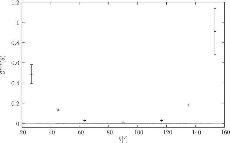
Figure 3: Comparison of the ILM prediction, Eqs. (3.19)–(3.20), with the lattice data for the “$zzz/zyy$” configuration at $|\vec{z}_{\perp}|=0\,{\rm fm}$. Here and in the following figures the dotted line corresponds to $n_{q}=1.33\,{\rm fm}^{-4}$ and the dashed line corresponds to $n_{q}=1.64\,{\rm fm}^{-4}$, with $\rho_{q}=0.35\,{\rm fm}$; the solid line corresponds to the phenomenological values $n=1\,{\rm fm}^{-4}$ and $\rho=1/3\,{\rm fm}$.

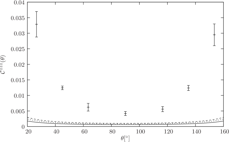
Figure 4: Same comparison as in Fig. 3 for the “$zzz$” configuration at $|\vec{z}_{\perp}|=0.1\,{\rm fm}$.

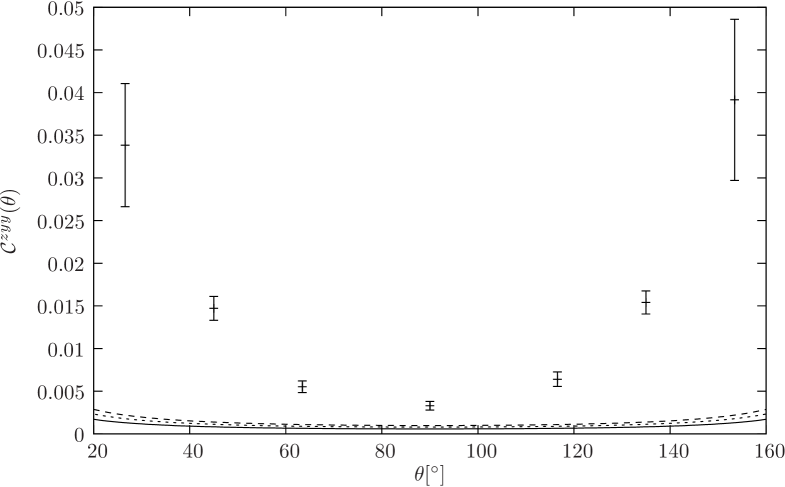
Figure 5: Same comparison as in Fig. 3 for the “$zyy$” configuration at $|\vec{z}_{\perp}|=0.1\,{\rm fm}$.

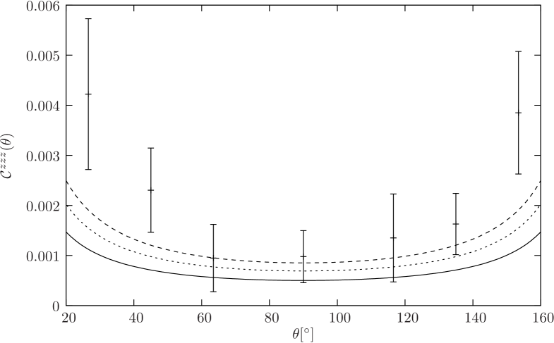
Figure 6: Same comparison as in Fig. 3 for the “$zzz$” configuration at $|\vec{z}_{\perp}|=0.2\,{\rm fm}$.

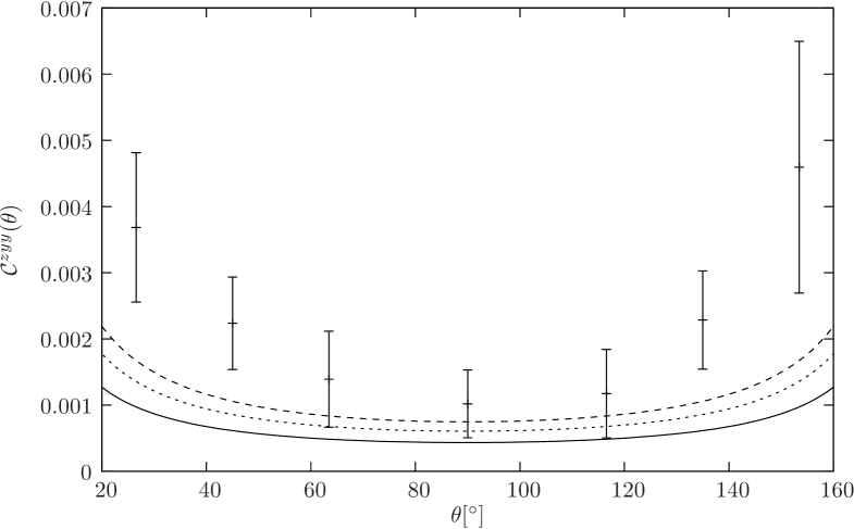
Figure 7: Same comparison as in Fig. 3 for the “$zyy$” configuration at $|\vec{z}_{\perp}|=0.2\,{\rm fm}$.

In order to compare the analytic expression (3.19) to the lattice data, we have to set the density $n$ and the radius $\rho$ to the appropriate values. The phenomenological estimates $n=1\,{\rm fm}^{-4}$ and $\rho=1/3\,{\rm fm}$ correspond to the physical (i.e., unquenched) case, while our numerical simulations have been performed in the quenched approximation of QCD, neglecting dynamical–fermion effects. We have then preferred to use the values $n_{q}=1.33$–$1.64\,{\rm fm}^{-4}$ for the density and $\rho_{q}=0.35\,{\rm fm}$ for the average size of the pseudoparticles, obtained directly by lattice calculations in the pure–gauge theory [39]. The packing fraction is a factor $1.6$–$2$ larger than the one obtained with the phenomenological values, but it is still a small number ($\lesssim 0.1$), so that the dilute liquid picture is still reasonable. The ILM prediction obtained with these values is shown in Figs. 3–7, together with the results obtained on the lattice in Ref. [28], for the loop configurations “$zzz$” ($\vec{R}_{1\perp}\parallel\vec{R}_{2\perp}\parallel\vec{z}_{\perp}$) and “$zyy$” ($\vec{R}_{1\perp}\parallel\vec{R}_{2\perp}\perp\vec{z}_{\perp}$), with $|\vec{R}_{1\perp}|=|\vec{R}_{2\perp}|=0.1\,{\rm fm}$. The dotted line corresponds to $n_{q}=1.33\,{\rm fm}^{-4}$, while the dashed line corresponds to $n_{q}=1.64\,{\rm fm}^{-4}$; for comparison, we plot also the prediction obtained using the phenomenological values of $n$ and $\rho$ (solid line). As already noticed in [28], the functional form does not seem to be the correct one to properly describe the lattice data, and a second term, proportional to $(\cot\theta)^{2}$, must be added to obtain a good fit. In Table 1 we show for comparison the ILM prediction of the prefactor $K=n_{q}({2}/{N_{c}})^{2}F(\vec{z}_{\perp},\vec{R}_{1\perp},\vec{R}_{2\perp})$, and the value obtained with a fit to the lattice data with the fitting functions (see Ref. [28])

$$f_{\rm ILM}=K_{\rm ILM}\frac{1}{\sin\theta},\qquad f_{\rm ILMp}=K_{\rm ILMp}\frac{1}{\sin\theta}+K_{\rm ILMp}^{\prime}(\cot\theta)^{2},$$ (3.21)

where $f_{\rm ILMp}$ is obtained by adding the lowest–order perturbative expression [41, 15, 19] to the ILM contribution. Notice, however, that $K_{\rm ILMp}^{\prime}$ can also receive nonperturbative contributions from two–instanton effects [23].

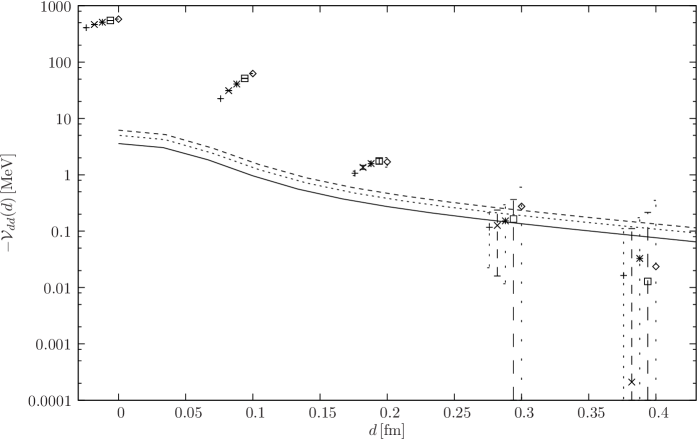
Figure 9: The instanton–induced dipole–dipole potential compared to the lattice data (on a logarithmic scale). The three lines correspond to $n_{q}=1.33\,{\rm fm}^{-4}$ (dotted line) and $n_{q}=1.64\,{\rm fm}^{-4}$ (dashed line) with $\rho_{q}=0.35\,{\rm fm}$, and to the phenomenological values $n=1\,{\rm fm}^{-4}$ and $\rho=1/3\,{\rm fm}$ (solid line). Here $\vec{R}_{1}=\vec{R}_{2}$ are parallel to $\vec{d}$, with $|\vec{R}_{i}|=0.1\,{\rm fm}$.

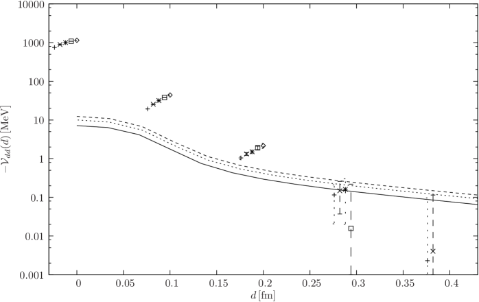
Figure 10: Same comparison as in Fig. 9, but with $\vec{R}_{1}=-\vec{R}_{2}$, $\vec{R}_{1}$ parallel to $\vec{d}$, with $|\vec{R}_{i}|=0.1\,{\rm fm}$.

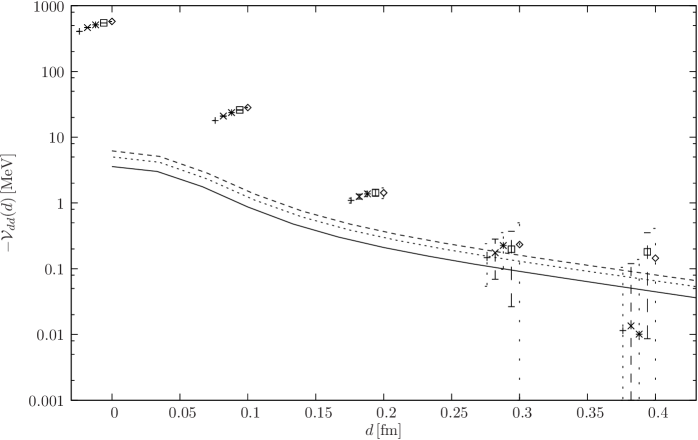
Figure 11: Same comparison as in Fig. 9, but with $\vec{R}_{1}=\vec{R}_{2}$ orthogonal to $\vec{d}$, with $|\vec{R}_{i}|=0.1\,{\rm fm}$.

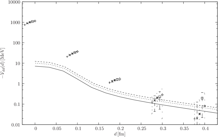
Figure 12: Same comparison as in Fig. 9, but with $\vec{R}_{1}=-\vec{R}_{2}$ orthogonal to $\vec{d}$, with $|\vec{R}_{i}|=0.1\,{\rm fm}$.

The instanton prediction turns out to be more or less of the correct order of magnitude in the range of distances considered, at least around $\theta=\pi/2$ [where, as we have said before, the one–instanton approximation used to derive the result, Eqs. (3.19) and (3.20), is expected to make sense], but it does not match the lattice data properly. The agreement with the data seems to be quite good at $|\vec{z}_{\perp}|=0.2\,{\rm fm}$; however, concerning the dependence on the relative distance between the loops, it seems that the ILM overestimates the correlation length which sets the scale for the rapid decrease of the correlation function. This is also supported by the comparison of the instanton–induced dipole–dipole potential, which we calculate in the next Section, with some preliminary numerical results on the lattice, as we show in Figs. 9–12.

4 Wilson–loop correlation function and the dipole–dipole potential

In this Section we calculate the normalised correlation function of two (infinite) parallel Wilson loops, which describe the time evolution of two static colour dipoles. The one–instanton approximation makes no sense here, since the interaction region has infinite extension in the time direction, and the effect of a whole time–series of pseudoparticles on the two dipoles has to be considered. The above–mentioned correlation function can be used to extract the dipole–dipole potential ${\cal V}_{dd}$ by means of the formula [29]

$$\dfrac{\langle{\cal W}_{1}{\cal W}_{2}\rangle}{\langle{\cal W}_{1}\rangle\langle{\cal W}_{2}\rangle}\mathop{\simeq}_{T\to\infty}e^{-T{\cal V}_{dd}(\vec{d},\vec{R}_{1},\vec{R}_{2})},$$ (4.1)

where $\vec{R}_{1}$ and $\vec{R}_{2}$ are the sizes of the two dipoles, $\vec{d}$ is the distance between their centers, and $T$ is the length of the two loops. Neglecting again the transverse connectors, the loops ${\cal W}_{1,2}$ are written as

$${\cal W}_{i}=\frac{1}{N_{c}}{\rm Tr}\,[{\rm W}^{(-){\dagger}}_{i}{\rm W}^{(+)}_{i}],$$ (4.2)

with

$${\rm W}^{(\pm)}_{1} ={\cal P}\exp\left[-ig\int_{0}^{T}A_{4}(ut+d\pm R_{1}/2)\,dt\right],$$ (4.3)

$${\rm W}^{(\pm)}_{2} ={\cal P}\exp\left[-ig\int_{0}^{T}A_{4}(ut\pm R_{2}/2)\,dt\right],$$

where $u=(\vec{0},1)$, $R_{i}=(\vec{R}_{i},0)$, $d=(\vec{d},0)$. To evaluate their correlation function [the numerator in (4.1)] we divide space–time into time–slices, and, in turn, the time–slices into cells; the procedure is the same as for the expectation value of a single loop, but this time we determine the spatial size $V^{(3)}_{\rm cell}$ to be large enough to accommodate both the dipoles. Requiring

$$V_{\rm cell}^{(3)}\sim\left(|\vec{d}|+\frac{|\vec{R}_{1}|+|\vec{R}_{2}|}{2}+2\rho\right)\left(\frac{|\vec{R}_{1}|+|\vec{R}_{2}|}{2}+2\rho\right)^{2},$$ (4.4)

we have to set $\delta T$ to

$$\frac{\delta T}{\rho} \sim 4, {\rm for}\,|\vec{d}|,|\vec{R}_{i}|\sim\rho/2,~{}~{}~{}~{}~{}\frac{\delta T}{\rho} \sim 2.5, {\rm for}\,|\vec{d}|,|\vec{R}_{i}|\sim\rho,$$ (4.5)

which is still a fairly large value. Note however that we are overestimating the volume of the region of 3–space where a pseudoparticle can affect the loop, so that $\delta T$ is actually underestimated. Again, for large distances the two dipoles interact with different pseudoparticles, and the correlation function is expected to factorise, thus giving a vanishing dipole–dipole potential as $|\vec{d}|\to\infty$.

Now let $K$ be the average number of instantons that interact with the loop. This number grows linearly with the length $T$ of the loop due to the uniformity of the liquid, and we can take, without loss of generality, $T=K\delta T$, since we are interested in the limit $T\to\infty$. We divide space–time into cells as described above, labelling $D_{1},\ldots,D_{K}$ the cells where the loop lives, and we define

$${\rm W}^{(\pm)}_{1}(k) ={\cal P}\exp\left[-ig\int_{(k-1)\delta T}^{k\delta T}A_{4}(ut+d\pm R_{1}/2)\,dt\right],$$ (4.6)

$${\rm W}^{(\pm)}_{2}(k) ={\cal P}\exp\left[-ig\int_{(k-1)\delta T}^{k\delta T}A_{4}(ut\pm R_{2}/2)\,dt\right],\quad k=1,\ldots,K,$$

and the “two–link” variables

$$\mathbb{T}_{i}(k) ={\rm W}^{(-)*}_{i}(k)\otimes{\rm W}^{(+)}_{i}(k),\qquad\mathbb{W}_{i}(j) =\prod_{k=j}^{1}\mathbb{T}_{i}(k),$$ (4.7)

which allow us to write

$${\cal W}_{i}=\frac{1}{N_{c}}\left[\mathbb{W}_{i}(K)\right]_{ijij}=\frac{1}{N_{c}}\widetilde{\rm Tr}\,\mathbb{W}_{i}(K).$$ (4.8)

The integration over the colour degrees of freedom of the pseudoparticles is more complicated than in the case of a single loop, although the procedure is the same. Starting from the $K$–th pseudoparticle, we have to calculate the integral

(4.9)

(4.10)

where

$$\begin{aligned} w_{i}(k)&\equiv\frac{1}{N_{c}}\hat{\mathbb{T}}_{i}(k)_{j^{\prime}_{1}j^{\prime}_{1}}|_{s}=\frac{1}{N_{c}}{\rm Tr}\,[{\rm W}^{(-){\dagger}}_{i}(k){\rm W}^{(+)}_{i}(k)]|_{s}=1-\frac{2}{N_{c}}\Delta_{i}(z_{P(k)}),\\ \Delta_{i}(z)&=1-\cos\alpha_{i+}\cos\alpha_{i-}-\hat{n}_{i+}\cdot\hat{n}_{i-}\sin\alpha_{i+}\sin\alpha_{i-},\\ \alpha_{i\pm}&=\frac{\pi\|n_{i\pm}\|}{\sqrt{\|n_{i\pm}\|^{2}+\rho^{2}}},\quad n^{a}_{1\pm}=-(d\pm\frac{R_{1}}{2}-z)_{a},\quad n^{a}_{2\pm}=-(\pm\frac{R_{2}}{2}-z)_{a},\end{aligned}$$ (4.11)

and we have introduced the quantities

$$\underline{w}_{12}(k)\equiv\frac{1}{N_{c}}\hat{\mathbb{T}}_{1}(k)_{j^{\prime}_{1}j^{\prime}_{2}}|_{s}\hat{\mathbb{T}}_{2}(k)_{j^{\prime}_{2}j^{\prime}_{1}}|_{s}=\frac{1}{N_{c}}{\rm Tr}\,[{\rm W}^{(-){\dagger}}_{1}(k){\rm W}^{(+)}_{1}(k){\rm W}^{(-){\dagger}}_{2}(k){\rm W}^{(+)}_{2}(k)]|_{s},$$

$$\overline{\mathbb{W}}_{12}(k)\equiv\check{\mathbb{W}}_{1}(k)_{j_{1}j_{2}}\check{\mathbb{W}}_{2}(k)_{j_{2}j_{1}}.$$ (4.12)

The effect of a single instanton on ${\rm W}^{(\pm)}_{i}(k)$ is given by

$${\rm W}_{i}^{(\pm)}=\left(\begin{array}[]{cc}\hskip 2.84526pt\exp\left[i\hat{n}^{a}_{i\pm}\sigma^{a}\alpha_{i\pm}\right]&\hskip 2.84526pt0\vspace{1mm}\\ \hskip 2.84526pt0&\hskip 2.84526pt\mathbb{I}_{N_{c}-2}\end{array}\right),$$ (4.15)

where $\mathbb{I}_{M}$ is the $M$-dimensional unit matrix, while the effect of an anti–instanton is obtained by replacing $n_{i\pm}\to-n_{i\pm}$. The expectation value of the quantity

$$\overline{\cal W}_{12}\equiv\frac{1}{N_{c}}\overline{\mathbb{W}}_{12}(K)=\frac{1}{N_{c}}{\rm Tr}\,[{\rm W}^{(-){\dagger}}_{2}{\rm W}^{(+)}_{1}{\rm W}^{(-){\dagger}}_{1}{\rm W}^{(+)}_{2}]$$ (4.16)

can be interpreted as the transition amplitude of an inelastic process, the final state $\widetilde{d}\widetilde{d}$ being the initial one, $dd$, with the (say) antiquarks in the two dipoles interchanged (see Fig. 8). Over the time $T$ a certain number of such transitions can happen, and this is at the origin of the new terms in the formulas above.

To proceed we also need to calculate the integral

$${\cal I}_{2}\equiv\int dU(K)\overline{\mathbb{W}}_{12}(K).$$ (4.17)

If we write

$$\overline{\mathbb{W}}_{12}(K)=\check{\mathbb{W}}_{1}(K)_{j_{1}j_{2}}\check{\mathbb{W}}_{2}(K)_{j_{2}j_{1}}=[\mathbb{T}_{1}(K)]_{j_{1}j^{\prime}_{1}j_{2}k^{\prime}_{1}}|_{s}[\mathbb{T}_{2}(K)]_{j_{2}j^{\prime}_{2}j_{1}k^{\prime}_{2}}|_{s}$$ (4.18)

$$\times U_{j_{1}j^{\prime}_{1}}U^{\dagger}_{k^{\prime}_{1}k_{1}}U_{j_{2}j^{\prime}_{2}}U^{\dagger}_{k^{\prime}_{2}k_{2}}\check{\mathbb{W}}_{1}(K-1)_{j_{1}k_{1}}\check{\mathbb{W}}_{2}(K-1)_{j_{2}k_{2}},$$

we find the same Haar integral as before, and thus, after contracting the colour indices, we find

$${\cal I}_{2}=aN_{c}\big{[}\overline{w}_{12}(K)-\widetilde{w}_{1}(K)\widetilde{w}_{2}(K)\big{]}\widetilde{\rm Tr}\,{\mathbb{W}}_{1}(K-1)\widetilde{\rm Tr}\,{\mathbb{W}}_{2}(K-1)$$ (4.19)

$$\phantom{unbelpezzounbelpezzo}+a\big{[}N_{c}^{2}\widetilde{w}_{1}(K)\widetilde{w}_{2}(K)-\overline{w}_{12}(K)\big{]}\overline{\mathbb{W}}_{12}(K-1),$$

where we have introduced the quantity $\overline{w}_{12}(k)$,

$$\overline{w}_{12}(k)\equiv\frac{1}{N_{c}}[\mathbb{T}_{1}(k)]_{j_{1}j^{\prime}_{1}j_{2}j^{\prime}_{1}}|_{s}[\mathbb{T}_{2}(k)]_{j_{2}j^{\prime}_{2}j_{1}j^{\prime}_{2}}|_{s}$$ (4.20)

$$\phantom{unbelpezzounbelpezzo}=\frac{1}{N_{c}}{\rm Tr}\,[{\rm W}^{(+)}_{1}(k){\rm W}^{(-){\dagger}}_{1}(k){\rm W}^{(+)}_{2}(k){\rm W}^{(-){\dagger}}_{2}(k)]|_{s},$$

and the quantities $\widetilde{w}_{i}(k)$, which come from the contraction of

$$\widetilde{w}_{1}(k)\widetilde{w}_{2}(k)=\frac{1}{N_{c}^{2}}[\mathbb{T}_{1}(k)]_{j_{1}j^{\prime}_{1}j_{2}j^{\prime}_{2}}|_{s}[\mathbb{T}_{2}(k)]_{j_{2}j^{\prime}_{2}j_{1}j^{\prime}_{1}}|_{s},$$ (4.21)

and are equal to the value of the Wilson loops (of infinite length) obtained from ${\cal W}_{i}$ interchanging the antiquarks in the two dipoles, in the field of a single pseudoparticle:

$$\widetilde{w}_{1}(k) \equiv\frac{1}{N_{c}}{\rm Tr}\,[{\rm W}^{(-){\dagger}}_{2}(k){\rm W}^{(+)}_{1}(k)]|_{s}=1-\frac{2}{N_{c}}\widetilde{\Delta}_{1}(z_{P(k)}),$$ (4.22)

$$\widetilde{\Delta}_{1}(z) =1-\cos\alpha_{1+}\cos\alpha_{2-}-\hat{n}_{1+}\cdot\hat{n}_{2-}\sin\alpha_{1+}\sin\alpha_{2-},$$

$$\widetilde{w}_{2}(k) \equiv\frac{1}{N_{c}}{\rm Tr}\,[{\rm W}^{(-){\dagger}}_{1}(k){\rm W}^{(+)}_{2}(k)]|_{s}=1-\frac{2}{N_{c}}\widetilde{\Delta}_{2}(z_{P(k)}),$$

$$\widetilde{\Delta}_{2}(z) =1-\cos\alpha_{2+}\cos\alpha_{1-}-\hat{n}_{2+}\cdot\hat{n}_{1-}\sin\alpha_{2+}\sin\alpha_{1-},$$

where the functions $\widetilde{\Delta}_{i}$ are again independent of the pseudoparticle species. Also, $\overline{w}_{12}(k)$ is related to $\underline{w}_{12}(k)$ in the same way.

To iterate the process we organise the previous results as follows:

$$\int dU(K) \left(\begin{array}[]{c}\widetilde{\rm Tr}\,{\mathbb{W}}_{1}(K)\widetilde{\rm Tr}\,{\mathbb{W}}_{2}(K)\vspace{1mm}\\ \overline{\mathbb{W}}_{12}(K)\end{array}\right)$$ (4.23)

$$\phantom{unbelpezzo}=M(K)\left(\begin{array}[]{c}\widetilde{\rm Tr}\,{\mathbb{W}}_{1}(K-1)\widetilde{\rm Tr}\,{\mathbb{W}}_{2}(K-1)\vspace{1mm}\\ \overline{\mathbb{W}}_{12}(K-1)\end{array}\right),$$

where $M(k)$ is the matrix

$$M(k)=\frac{1}{N_{c}^{2}-1}\left(\begin{array}[]{cc}N_{c}^{2}w_{1}(k)w_{2}(k)-\underline{w}_{12}(k)&N_{c}\big{[}\underline{w}_{12}(k)-w_{1}(k)w_{2}(k)\big{]}\vspace{1.5mm}\\ N_{c}\big{[}\overline{w}_{12}(k)-\widetilde{w}_{1}(k)\widetilde{w}_{2}(k)\big{]}&N_{c}^{2}\widetilde{w}_{1}(k)\widetilde{w}_{2}(k)-\overline{w}_{12}(k)\end{array}\right).$$ (4.26)

The iteration is now straightforward, and yields

$$\int d^{K}U \left(\begin{array}[]{c}N_{c}^{2}{\cal W}_{1}{\cal W}_{2}\vspace{1mm}\\ N_{c}\overline{\cal W}_{12}\end{array}\right)$$ (4.27)

$$= \int d^{K}U\left(\begin{array}[]{c}\widetilde{\rm Tr}\,{\mathbb{W}}_{1}(K)\widetilde{\rm Tr}\,{\mathbb{W}}_{2}(K)\vspace{1mm}\\ \overline{\mathbb{W}}_{12}(K)\end{array}\right)=\left[\prod_{k=K}^{1}M(k)\right]\left(\begin{array}[]{c}N_{c}^{2}\vspace{1.5mm}\\ N_{c}\end{array}\right),$$

where we used the fact that

$$\left(\begin{array}[]{c}\widetilde{\rm Tr}\,{\mathbb{W}}_{1}(1)\widetilde{\rm Tr}\,{\mathbb{W}}_{2}(1)\vspace{1mm}\\ \overline{\mathbb{W}}_{12}(1)\end{array}\right)\bigg{|}_{s}=\left(\begin{array}[]{c}{N_{c}^{2}}w_{1}(1)w_{2}(1)\vspace{1.5mm}\\ {N_{c}}\overline{w}_{12}(1)\end{array}\right)=M(1)\left(\begin{array}[]{c}N_{c}^{2}\vspace{1.5mm}\\ N_{c}\end{array}\right).$$ (4.34)

We are left with the integration over the pseudoparticle positions. The procedure is described in Appendix B; using Eq. (B.7) we then obtain

$$\int d^{4N}z\,{\cal D}(\{z\})\left[\prod_{k=K}^{1}M(k)\right]=\prod_{j=K}^{1}n\int_{D_{j}}d^{4}z\,\Big{(}\nu_{{\rm I}}M(z,\sigma_{{\rm I}})+\nu_{\bar{\rm I}}M(z,\sigma_{\bar{\rm I}})\Big{)}$$ (4.35)

$$=\prod_{j=K}^{1}\left[\mathbb{I}_{2}+n\int_{D_{j}}d^{4}z\,\Big{(}\nu_{{\rm I}}\hat{M}(z,\sigma_{{\rm I}})+\nu_{\bar{\rm I}}\hat{M}(z,\sigma_{\bar{\rm I}})\Big{)}\right],$$

where $\hat{M}\equiv M-\mathbb{I}_{2}$ falls off to zero as $|z|\to\infty$, and where $\nu_{{\rm I},\bar{\rm I}}\equiv n_{{\rm I},\bar{\rm I}}/n$. Performing the trivial integration over the time position, extending the spatial integration to the whole space, and letting (formally) $K\to\infty$ with $T$ fixed, we obtain

$$\int d^{4N}z\,{\cal D}(\{z\})\left[\prod_{k=K}^{1}M(k)\right]=\exp\{nT{\cal J}\},$$ (4.36)

where the matrix ${\cal J}$ is given by

$${\cal J} \equiv\int d^{3}z\Big{(}\nu_{{\rm I}}\hat{M}(z,\sigma_{{\rm I}})+\nu_{\bar{\rm I}}\hat{M}(z,\sigma_{\bar{\rm I}})\Big{)}=\frac{1}{N_{c}^{2}-1}\left(\begin{array}[]{cc}N_{c}^{2}A-B&N_{c}(B-A)\vspace{1mm}\\ N_{c}(\widetilde{B}-\widetilde{A})&N_{c}^{2}\widetilde{A}-\widetilde{B}\end{array}\right)$$ (4.39)

$$=\left(\begin{array}[]{cc}B&0\vspace{1mm}\\ 0&\widetilde{B}\end{array}\right)+\frac{1}{N_{c}^{2}-1}\left(\begin{array}[]{cc}N_{c}^{2}(A-B)&N_{c}(B-A)\vspace{1mm}\\ N_{c}(\widetilde{B}-\widetilde{A})&N_{c}^{2}(\widetilde{A}-\widetilde{B})\end{array}\right),$$ (4.44)

having defined

$$A =\int d^{3}z\left[\left(\frac{2}{N_{c}}\right)^{2}\Delta_{1}(z)\Delta_{2}(z)-\frac{2}{N_{c}}\Delta_{1}(z)-\frac{2}{N_{c}}\Delta_{2}(z)\right],$$ (4.45)

$$\widetilde{A} =\int d^{3}z\left[\left(\frac{2}{N_{c}}\right)^{2}\widetilde{\Delta}_{1}(z)\widetilde{\Delta}_{2}(z)-\frac{2}{N_{c}}\widetilde{\Delta}_{1}(z)-\frac{2}{N_{c}}\widetilde{\Delta}_{2}(z)\right],$$

$$B =\int d^{3}z\,\bigg{[}\nu_{{\rm I}}(\underline{w}_{12}(z,{\rm I})-1)+\nu_{\bar{\rm I}}(\underline{w}_{12}(z,\bar{\rm I})-1)\bigg{]},$$

$$\widetilde{B} =\int d^{3}z\,\bigg{[}\nu_{{\rm I}}(\overline{w}_{12}(z,{\rm I})-1)+\nu_{\bar{\rm I}}(\overline{w}_{12}(z,\bar{\rm I})-1)\bigg{]}.$$

To proceed further with the calculation we now set the pseudoparticle fractions to their phenomenological values $\nu_{{\rm I}}=\nu_{\bar{\rm I}}=1/2$: in this case we can show that (see Appendix B)

$$B=\widetilde{B} =\frac{2}{N_{c}}\int d^{3}z\bigg{[}\big{(}\Delta_{1}(z)\Delta_{2}(z)+\widetilde{\Delta}_{1}(z)\widetilde{\Delta}_{2}(z)-\Delta_{+}(z)\Delta_{-}(z)\big{)}$$ (4.46)

$$\phantom{unbe}-\big{(}\Delta_{1}(z)+\Delta_{2}(z)+\widetilde{\Delta}_{1}(z)+\widetilde{\Delta}_{2}(z)-\Delta_{+}(z)-\Delta_{-}(z)\big{)}\bigg{]},$$

where the quantities

$${\Delta}_{+}(z) =1-\cos\alpha_{1+}\cos\alpha_{2+}-\hat{n}_{1+}\cdot\hat{n}_{2+}\sin\alpha_{1+}\sin\alpha_{2+},$$ (4.47)

$${\Delta}_{-}(z) =1-\cos\alpha_{2-}\cos\alpha_{1-}-\hat{n}_{2-}\cdot\hat{n}_{1-}\sin\alpha_{2-}\sin\alpha_{1-},$$

are the analogues of $\widetilde{\Delta}_{i}$ with the positions of the quark and the antiquark in the (say) second dipole interchanged. It is now easy to diagonalise ${\cal J}$: denoting with $X=A-B$, $\widetilde{X}=\widetilde{A}-B$, the eigenvalues can be written as

$${\lambda}_{\pm}=\frac{A+\widetilde{A}}{2}+\frac{1}{2(N_{c}^{2}-1)}\left\{X+\widetilde{X}\pm N_{c}\sqrt{(N_{c}^{2}-1)(\widetilde{X}-X)^{2}+(\widetilde{X}+X)^{2}}\right\};$$ (4.48)

since they are different, ${\cal J}$ is diagonalisable. Denoting by $\Pi_{\pm}$ the corresponding projectors we can write [$v_{0}\equiv(1,0)$, $v_{N_{c}}\equiv(N_{c}^{2},N_{c})$]

$$N_{c}^{2}\langle{\cal W}_{1}{\cal W}_{2}\rangle_{\rm ILM} =v_{0}\cdot\big{(}\exp\{nT{\cal J}\}v_{N_{c}}\big{)}$$ (4.49)

$$=v_{0}\cdot\left[\big{(}e^{nT\lambda_{+}}\Pi_{+}+e^{nT\lambda_{-}}\Pi_{-}\big{)}v_{N_{c}}\right],$$

and, taking the logarithm, in the large–$T$ limit we find

$$\log\langle{\cal W}_{1}{\cal W}_{2}\rangle_{\rm ILM}=nT\lambda_{+}+{\rm(subleading\,\,terms)}.$$ (4.50)

In the last passage we have implicitly assumed that the projector $\Pi_{+}$ is such that $v_{0}\cdot(\Pi_{+}v_{N_{c}})>0$: we have explicitly verified that this is true in the cases that we have investigated numerically. Note that the correlation function of parallel loops must be positive, as a consequence of reflection positivity of the Euclidean theory [43]: this can be easily proved following Ref. [44]. Finally, recalling Eqs. (4.1) and (2.11) we can conclude that

$${\cal V}_{dd}(\vec{d},\vec{R}_{1},\vec{R}_{2})={\cal V}_{12}(\vec{d},\vec{R}_{1},\vec{R}_{2})-{\cal V}_{q\bar{q}}(|\vec{R}_{1}|)-{\cal V}_{q\bar{q}}(|\vec{R}_{2}|),$$ (4.51)

where we have set ${\cal V}_{12}\equiv-n\lambda_{+}$.

In Figs. 9–12 we show the comparison of the instanton–induced dipole–dipole potential with some preliminary numerical data obtained on the lattice: to our knowledge, lattice measurements of this quantity are not present in the literature. Also in this case we have performed a quenched $SU(3)$ lattice calculation, with the same parameters ($16^{4}$ hypercubic lattice, $\beta=6.0$) used in Ref. [28], and so we have to use the quenched instanton density $n_{q}$ and radius $\rho_{q}$, as explained in the previous Section. The errors are very large for the lattice data corresponding to the largest distances and lengths, and a plateau has not been reached yet even at $T=0.8\,{\rm fm}$ at $|\vec{d}\,|=0\,{\rm fm}$ and $|\vec{d}\,|=0.1\,{\rm fm}$. However, we believe that the order of magnitude will not change much for larger lengths: in the various plots we show the available values for ${\cal V}_{dd}$ as obtained with loops of increasing lengths ($0.4\div 0.8\,{\rm fm}$), by means of Eq. (4.1), and indeed on a logarithmic scale they seem to be quite stable. The lattice value of ${\cal V}_{dd}$ extracted from the largest–length loops is plotted at the correct value of the distance, while the data points corresponding to shorter lengths are slightly shifted, with the length increasing from left to right. The instanton–induced potential and the lattice data have different orders of magnitude for the shortest distances. At larger distances there seems to be a better agreement, but the error bars of the lattice data are very large there, and a better precision is needed to quantify the importance of instanton effects at large distances. However, as already noticed in the previous Section, the rate of decrease with the distance seems to be underestimated in the ILM, which would lead to an increasing discrepancy between the prediction and the lattice data as the distance between the dipoles increases.

5 Conclusions

In this paper we have considered instanton effects, in the framework of the ILM, on the Wilson–loop correlation function relevant to soft high–energy scattering, and we have compared the results to the lattice data discussed in Ref. [28]. Using an approximate density function, we have critically repeated the ILM calculation of the relevant correlation function, already performed in Ref. [23], properly taking into account effects which were neglected in that paper. The analytic dependence on the angular variable $\theta$ is the same as the one found in Ref. [23], which we have used in Ref. [28] to perform fits to the lattice data. In this paper we have instead performed a direct comparison of the ILM quantitative prediction, obtained by evaluating numerically our analytic expression for the loop–loop correlation function in the relevant cases. In doing so, we have used the pseudoparticle density $n_{q}$ and radius $\rho_{q}$ appropriate for the quenched approximation of QCD, in which the lattice calculation has been performed. A direct numerical comparison allows us to test not only the given functional form, but also the quantitative relevance of instanton effects on the Wilson–loop correlation function.

The comparison of the ILM prediction with the lattice data is not satisfactory, although it seems to have the correct shape in the vicinity of $\theta=90^{\circ}$. Moreover, although the ILM prediction seems to be (more or less) of the correct order of magnitude, the rate of decrease with the transverse distance seems to be underestimated. Here one sees the importance of a quantitative comparison: terms behaving as $1/\sin\theta$ (which are qualitatively good in fitting the data around $\theta=90^{\circ}$) can have a different origin than instantons, and indeed it seems that the ILM is not able to explain them from a quantitative point of view. Also, the ILM expression cannot account for the small but non–zero odderon contribution to the correlation function which we have found in the lattice results [28]. As a final remark, note that, after analytic continuation into Minkowski space–time, the ILM result in the one–instanton approximation gives an exactly zero total cross section, since the forward meson–meson scattering amplitude turns out to be purely real. The situation can change after inclusion of two–instanton effects, which are expected to yield a constant total cross section at high energy [23]; nevertheless, an analytic expression for this contribution is currently unavailable.

In this paper we have also derived an analytic expression for the instanton–induced dipole–dipole potential from the correlation function of two parallel Wilson loops, which we have compared to some preliminary data from the lattice. In this case, instanton effects seem to be negligible at short distances, less than or equal to the size of the dipoles, where there is a large discrepancy with the lattice results. The rate of decrease of the potential with the spatial distance between the dipoles predicted by the ILM seems also in this case to be smaller than the value found on the lattice; a better accuracy in the numerical calculations is needed to make this statement quantitative, but we think that the situation would not change from a qualitative point of view.

Appendix A Dependence of the Wilson–loop correlation function on the longitudinal momentum fractions

Exploiting the symmetries of the functional integral, one can show that the relevant Wilson–loop correlation function for given values of the longitudinal momentum fractions can always be reduced to the case $f_{1}=f_{2}=1/2$. We discuss here the case of the physical, Minkowskian correlation function ${\cal G}_{M}$; the proof in the Euclidean case is perfectly analogous.

As far as the dependence on the transverse vectors $\vec{z}_{\perp}$, $\vec{R}_{1\perp}$, and $\vec{R}_{2\perp}$, and on the longitudinal momentum fractions $f_{1}$ and $f_{2}$ is concerned, the invariance of the theory under translations and spatial rotations implies that ${\cal G}_{M}$ can depend only on the scalar products between the relative positions of quarks and antiquarks in transverse space. The number of independent variables is then six, while $\vec{z}_{\perp}$, $\vec{R}_{i\perp}$ and $f_{i}$ form a set of eight variables, so two of them are redundant. Indeed, the loop configuration in the transverse plane is determined by the relative distances $\vec{R}_{1\perp}$ and $\vec{R}_{2\perp}$ between quarks and antiquarks inside each meson, and by the relative distance between (say) quark 1 and quark 2 in the transverse plane,

$$\vec{X}^{1q}_{\perp}(\tau)-\vec{X}^{2q}_{\perp}(\tau)=\vec{z}_{\perp}+(1-f_{1})\vec{R}_{1\perp}-(1-f_{2})\vec{R}_{2\perp},\quad\forall\tau.$$ (A.1)

To determine which configurations are equivalent, we have to solve the equation

$$\vec{z}_{\perp}^{\,\prime}=\vec{z}_{\perp}+(f_{1}^{\prime}-f_{1})\vec{R}_{1\perp}-(f_{2}^{\prime}-f_{2})\vec{R}_{2\perp}.$$ (A.2)

Since a configuration specified by $(\vec{z}^{\,\prime}_{\perp},f_{1}^{\prime},f_{2}^{\prime})$, with $\vec{z}^{\,\prime}_{\perp}$ given above, is equivalent to the configuration $(\vec{z}_{\perp},f_{1},f_{2})$ we have

$${\cal G}_{M}(\chi;T;\vec{z}^{\,\prime}_{\perp};\vec{R}_{1\perp},f_{1}^{\prime},\vec{R}_{2\perp},f_{2}^{\prime})={\cal G}_{M}(\chi;T;\vec{z}_{\perp};\vec{R}_{1\perp},f_{1},\vec{R}_{2\perp},f_{2});$$ (A.3)

one can then choose a reference value for $f_{i}^{\prime}$, for example $f_{1}^{\prime}=f_{2}^{\prime}=1/2$, and move all the dependence on $f_{i}$ inside the dependence on the impact parameter. Moreover, since ${\cal G}_{M}$ enters the dipole–dipole scattering amplitude with its 2–dimensional Fourier transform with respect to the impact parameter, one can write

$$\int d^{2}z_{\perp}\,e^{i\vec{q}_{\perp}\cdot\vec{z}_{\perp}}{\cal G}_{M}(\chi;T;\vec{z}_{\perp};\vec{R}_{1\perp},f_{1},\vec{R}_{2\perp},f_{2})$$

$$= \int d^{2}z_{\perp}\,e^{i\vec{q}_{\perp}\cdot\vec{z}_{\perp}}{\cal G}_{M}(\chi;T;\vec{z}_{\perp}-(f_{1}-\frac{1}{2})\vec{R}_{1\perp}+(f_{2}-\frac{1}{2})\vec{R}_{2\perp};\vec{R}_{1\perp},\frac{1}{2},\vec{R}_{2\perp},\frac{1}{2})$$

$$= e^{i\vec{q}_{\perp}\cdot[(f_{1}-\frac{1}{2})\vec{R}_{1\perp}-(f_{2}-\frac{1}{2})\vec{R}_{2\perp}]}\int d^{2}z_{\perp}\,e^{i\vec{q}_{\perp}\cdot\vec{z}_{\perp}}{\cal G}_{M}(\chi;T;\vec{z}_{\perp};\vec{R}_{1\perp},\frac{1}{2},\vec{R}_{2\perp},\frac{1}{2}).$$ (A.4)

It is then clear that one can consider the case $f_{1}=f_{2}=1/2$ only. In particular, in the forward case, i.e., $\vec{q}_{\perp}=0$, the dependence on $f_{i}$ drops, and the integration on the longitudinal momentum fractions affects only the wave functions.

Appendix B Technical details

B.1 Integration over the position of pseudoparticles

Consider the integral

$${\cal I}\equiv\int d^{4N}z\,{\cal D}(\{z\})\prod_{k\in I_{K}}f_{k}(z_{P(k)},\sigma_{P(k)}),$$ (B.1)

where $f_{k}$ are $K$ (possibly distinct) matrices, whose entries are functions of the position and of the type of the pseudoparticle lying in cell $k$, and $I_{K}$ is the ordered set of the $K$ relevant cells. We have

$${\cal I}={\cal N}^{-1}\int d^{4N}z \,\left[\sum_{P}\prod_{j=1}^{N}\chi_{D_{j}}(z_{P(j)})\right]\prod_{k\in I_{K}}f_{k}(z_{P(k)},\sigma_{P(k)})$$ (B.2)

$$={\cal N}^{-1}\sum_{P}V_{\rm cell}^{N-K}\int d^{4K}z\prod_{k\in I_{K}}\chi_{D_{k}}(z_{P(k)})f_{k}(z_{P(k)},\sigma_{P(k)})$$

$$={\cal N}^{-1}\sum_{P}V_{\rm cell}^{N-K}\prod_{k\in I_{K}}\int_{D_{k}}d^{4}z\,f_{k}(z,\sigma_{P(k)}),$$

which, denoting

$$F_{k}(\sigma_{P(k)})\equiv\int_{D_{k}}d^{4}z\,f_{k}(z,\sigma_{P(k)}),$$ (B.3)

becomes

$${\cal I} ={\cal N}^{-1}\sum_{P}V_{\rm cell}^{N-K}\prod_{k\in I_{K}}F_{k}(\sigma_{P(k)})={\cal N}^{-1}\sum_{S_{K}}V_{\rm cell}^{N-K}\eta(S_{K})\prod_{k\in I_{K}}F_{k}(\sigma_{P(k)}),$$ (B.4)

where $\sum_{S_{K}}$ denotes the sum over all possible sequences of $K$ pseudoparticles, and $\eta(S_{K})$ is the number of ways in which a given sequence can be obtained from the ensemble,

$$\eta(S_{K})=(N-K)!\frac{N_{{\rm I}}!}{(N_{{\rm I}}-l_{{\rm I}})!}\frac{N_{\bar{\rm I}}!}{(N_{\bar{\rm I}}-l_{\bar{\rm I}})!},$$ (B.5)

$l_{{\rm I}}$ and $l_{\bar{\rm I}}$ being the number of instantons and anti–instantons in the sequence, respectively. In the limit of large $N_{{\rm I}}$, $N_{\bar{\rm I}}$ and $V$, with the ratios $\nu_{{\rm I}}=N_{{\rm I}}/N$, $\nu_{\bar{\rm I}}=N_{\bar{\rm I}}/N$, and $n=N/V$ kept fixed,

$$\eta(S_{K})\to{\cal N}n^{N}\nu_{{\rm I}}^{l_{{\rm I}}}\nu_{\bar{\rm I}}^{l_{\bar{\rm I}}},$$ (B.6)

and so Eq. (B.4) simplifies to (recall that $nV_{\rm cell}=1$)

$${\cal I} =n^{K}\sum_{S_{K}}\nu_{{\rm I}}^{l_{{\rm I}}}\nu_{\bar{\rm I}}^{l_{\bar{\rm I}}}\prod_{k\in I_{K}}F_{k}(\sigma_{P(k)})=n^{K}\sum_{S_{K}}\prod_{k\in I_{K}}\nu_{\sigma_{P(k)}}F_{k}(\sigma_{P(k)})$$ (B.7)

$$=n^{K}\prod_{k\in I_{K}}\sum_{\sigma={\rm I},\bar{\rm I}}\nu_{\sigma}F_{k}(\sigma)=\prod_{k\in I_{K}}n\sum_{\sigma={\rm I},\bar{\rm I}}\nu_{\sigma}\int_{D_{k}}d^{4}z\,f_{k}(z,\sigma).$$

B.2 The function $B$ for $\nu_{{\rm I}}=\nu_{\bar{\rm I}}$

We prove that the functions $B$ and $\widetilde{B}$, defined in Eq. (4.45), are equal for $\nu_{{\rm I}}=\nu_{\bar{\rm I}}$, and find their explicit form. To do so, note the following about $SU(2)$ matrices. One can always write ${\rm u}\in SU(2)$ as

$${\rm u}=u^{0}\mathbb{I}_{2}+i\vec{u}\cdot\vec{\sigma},\quad u^{0},u^{i}\in\mathbb{R},\quad(u^{0})^{2}+\vec{u}^{\,2}=1,$$ (B.8)

with $u^{0}={\rm Tr}_{2}\,{\rm u}$ and $\vec{u}=-i\,{\rm Tr}_{2}\,\vec{\sigma}{\rm u}$, with ${\rm Tr}_{2}\,\equiv(1/2){\rm Tr}\,$. Using the commutation and anticommutation relations satisfied by the Pauli matrices,

$$[\sigma_{i},\sigma_{j}] =2i\epsilon_{ijk}\sigma_{k},\quad\{\sigma_{i},\sigma_{j}\}=2\delta_{ij}\mathbb{I}_{2},$$ (B.9)

we can write for the product of two unitary matrices

$${\rm u}\equiv{\rm u}_{1}{\rm u}_{2}=u^{0}\mathbb{I}_{2}+i\vec{u}\cdot\vec{\sigma},$$ (B.10)

with

$$u^{0} =[(u_{1})^{0}(u_{2})^{0}-\vec{u}_{1}\cdot\vec{u}_{2}], \vec{u}_{\phantom{a}} =\vec{u}_{s}+\vec{u}_{a},$$ (B.11)

$$\vec{u}_{s} =(u_{1})^{0}\vec{u}_{2}+(u_{2})^{0}\vec{u}_{1}, \vec{u}_{a} =-(\vec{u}_{1}\wedge\vec{u}_{2}).$$

Clearly, if we interchange ${\rm u}_{1}$ and ${\rm u}_{2}$ we obtain

$${\rm v} \equiv{\rm u}_{2}{\rm u}_{1}={v}^{0}\mathbb{I}_{2}+i\vec{v}\cdot\vec{\sigma},$$ (B.12)

$$v^{0} =u^{0},\quad\vec{v}=\vec{u}_{s}-\vec{u}_{a}.$$

In our case, denoting with ${\rm w}_{i}^{(\pm)}(k)$ the non–trivial $2\times 2$ part of ${\rm W}^{(\pm)}_{i}(k)$, we have (suppressing the argument $k$)

$${\rm w}^{(\pm)}_{i}=w_{(\pm)i}^{0}\mathbb{I}_{2}+\vec{w}_{(\pm)i}\cdot\vec{\sigma},$$ (B.13)

so that

$${\rm w}_{i}\equiv{\rm w}^{(-){\dagger}}_{i}{\rm w}^{(+)}_{i} =w^{0}_{i}\mathbb{I}_{2}+(\vec{w}_{i;s}+\vec{w}_{i;a})\cdot\vec{\sigma},$$ (B.14)

where, explicitly,

$$w^{0}_{i} =[(w_{(-)i})^{0}(w_{(+)i})^{0}+\vec{w}_{(-)i}\cdot\vec{w}_{(+)i}],$$ (B.15)

$$\vec{w}_{i;s} =[(w_{(-)i})^{0}\vec{w}_{(+)i}-(w_{(+)i})^{0}\vec{w}_{(-)i}],$$

$$\vec{w}_{i;a} =\vec{w}_{(-)i}\wedge\vec{w}_{(+)i}\,.$$

Since the vectors $\vec{w}_{(\pm)i}$ change sign if we replace an instanton with an anti–instanton, we have that under this replacement $\vec{w}_{i;s}$ changes sign, too, while $\vec{w}_{i;a}$ does not. Letting $\widetilde{\rm w}_{1}={\rm w}^{(-){\dagger}}_{2}{\rm w}^{(+)}_{1}$ and $\widetilde{\rm w}_{2}={\rm w}^{(-){\dagger}}_{1}{\rm w}^{(+)}_{2}$, and $\bar{\rm w}_{i}={\rm w}^{(+)}_{i}{\rm w}^{(-){\dagger}}_{i}$, we have

$$1-\underline{w}_{12} =\frac{2}{N_{c}}\{1-{\rm Tr}_{2}\,[{\rm w}_{1}{\rm w}_{2}]\},$$ (B.16)

$$1-\overline{w}_{12} =\frac{2}{N_{c}}\{1-{\rm Tr}_{2}\,[\widetilde{\rm w}_{1}\widetilde{\rm w}_{2}]\}=\frac{2}{N_{c}}\{1-{\rm Tr}_{2}\,[\bar{\rm w}_{1}\bar{\rm w}_{2}]\};$$

now,

$${\rm Tr}_{2}\,[{\rm w}_{1}{\rm w}_{2}] =w^{0}_{1}w^{0}_{2}-(\vec{w}_{1;s}+\vec{w}_{1;a})\cdot(\vec{w}_{2;s}+\vec{w}_{2;a}),$$ (B.17)

$${\rm Tr}_{2}\,[\bar{\rm w}_{1}\bar{\rm w}_{2}] =w^{0}_{1}w^{0}_{2}-(\vec{w}_{1;s}-\vec{w}_{1;a})\cdot(\vec{w}_{2;s}-\vec{w}_{2;a}),$$

and since we are averaging with equal weights over the pseudoparticle species, we need to consider only terms which are symmetric under ${\rm I}\leftrightarrow\bar{\rm I}$,

$${\rm Tr}_{2}\,[{\rm w}_{1}{\rm w}_{2}] =w^{0}_{1}w^{0}_{2}-(\vec{w}_{1;s}\cdot\vec{w}_{2;s}+\vec{w}_{1;a}\cdot\vec{w}_{2;a})+\,{\rm antisymmetric\,\,terms},$$ (B.18)

$${\rm Tr}_{2}\,[\bar{\rm w}_{1}\bar{\rm w}_{2}] =w^{0}_{1}w^{0}_{2}-(\vec{w}_{1;s}\cdot\vec{w}_{2;s}+\vec{w}_{1;a}\cdot\vec{w}_{2;a})+\,{\rm antisymmetric\,\,terms}.$$

From its definition, Eq. (4.45), it is now immediate to conclude that $B=\widetilde{B}$. Moreover, one can show that

$$\vec{w}_{1;s}\cdot\vec{w}_{2;s}+\vec{w}_{1;a}\cdot\vec{w}_{2;a}$$ (B.19)

$$=[(w_{(+)1})^{0}(w_{(+)2})^{0}+\vec{w}_{(+)1}\cdot\vec{w}_{(+)2}][(w_{(-)1})^{0}(w_{(-)2})^{0}+\vec{w}_{(-)1}\cdot\vec{w}_{(-)2}]$$

$$-[(w_{(-)1})^{0}(w_{(+)2})^{0}+\vec{w}_{(-)1}\cdot\vec{w}_{(+)2}][(w_{(-)2})^{0}(w_{(+)1})^{0}+\vec{w}_{(-)2}\cdot\vec{w}_{(+)1}],$$

which introducing

$${\rm w}_{+} ={\rm w}_{1}^{(+){\dagger}}{\rm w}_{2}^{(+)}={w}_{+}^{0}\mathbb{I}_{2}+i\vec{w}_{+}\cdot\vec{\sigma},$$ (B.20)

$${\rm w}_{-} ={\rm w}_{1}^{(-){\dagger}}{\rm w}_{2}^{(-)}={w}_{-}^{0}\mathbb{I}_{2}+i\vec{w}_{-}\cdot\vec{\sigma},$$

leads to

$${\rm Tr}_{2}\,[{\rm w}_{1}{\rm w}_{2}]|_{\rm symmetric} =w^{0}_{1}w^{0}_{2}+\widetilde{w}^{0}_{1}\widetilde{w}^{0}_{2}-w^{0}_{+}w^{0}_{-}={\rm Tr}_{2}\,[\widetilde{\rm w}_{1}\widetilde{\rm w}_{2}]|_{\rm symmetric},$$ (B.21)

and thus to

$$B=\int d^{3}z\,\frac{1}{2}\big{[}\big{(}\underline{w}_{12}(z,{\rm I})-1\big{)}+\big{(}\underline{w}_{12}(z,\bar{\rm I})-1\big{)}\big{]}=\frac{2}{N_{c}}\int d^{3}z\,\big{[}\big{(}\Delta_{1}\Delta_{2}$$ (B.22)

$$+\widetilde{\Delta}_{1}\widetilde{\Delta}_{2}-\Delta_{+}\Delta_{-}\big{)}-\big{(}\Delta_{1}+\Delta_{2}+\widetilde{\Delta}_{1}+\widetilde{\Delta}_{2}-\Delta_{+}-\Delta_{-}\big{)}\big{]}=\widetilde{B},$$

with $\Delta_{\pm}$ given in the text, Eq. (4.47).

	predicted		fitted–ILM		fitted–ILMp
$|\vec{z}_{\perp}|\,[{\rm fm}]$	$zzz$	$zyy$	$zzz$	$zyy$	$zzz$	$zyy$
0.0	0.880–1.08	0.880–1.08	17.1	17.1	9.86	9.86
0.1	0.827–1.02	0.798–0.984	7.60	5.79	4.32	3.39
0.2	0.692–0.853	0.607–0.748	1.31	1.43	0.947	1.14

Table 1: Value of $K_{\rm ILM}\times 10^{3}$ for the relevant configurations: ILM prediction (first column), “ILM” fit (second column) and “ILMp” fit (third column).

Figure 8: Schematic representation of the operators ${\cal W}_{1}{\cal W}_{2}$ (left) and $\overline{\cal W}_{12}$ (right), corresponding respectively to the processes $dd\to dd$ and $dd\to\widetilde{d}\widetilde{d}$. White (black) circles represent quarks (antiquarks).

References

- [1] A.A. Belavin, A.M. Polyakov, A.S. Schwartz and Yu.S. Tyupkin, Phys. Lett. B 59 (1975) 85.
- [2] R. Jackiw and C. Rebbi, Phys. Rev. Lett. 37 (1976) 172.
- [3] C.G. Callan, R. Dashen and D.J. Gross, Phys. Lett. B 63 (1976) 334.
- [4] A.M. Polyakov, Nucl. Phys. B 120 (1977) 429.
- [5] G. ’t Hooft, Phys. Rev. Lett. 37 (1976) 8; G. ’t Hooft, Phys. Rev. D 14 (1976) 3432; (erratum) Phys. Rev. D 18 (1978) 2199.
- [6] C.G. Callan, R. Dashen and D.J. Gross, Phys. Rev. D 17 (1978) 2717.
- [7] M.F. Atiyah, N.J. Hitchin, V.G. Drinfeld and Yu.I. Manin, Phys. Lett. A 65 (1978) 185.
- [8] E.V. Shuryak, Nucl. Phys. B. 203 (1982) 93; 116; 140.
- [9] T. Schäfer and E.V. Shuryak, Rev. Mod. Phys. 70 (1998) 323.
- [10] O. Nachtmann, Ann. Phys. 209 (1991) 436.
- [11] H.G. Dosch, E. Ferreira and A. Krämer, Phys. Rev. D 50 (1994) 1992.
- [12] O. Nachtmann, in Perturbative and Nonperturbative aspects of Quantum Field Theory, edited by H. Latal and W. Schweiger (Springer–Verlag, Berlin, Heidelberg, 1997).
- [13] E.R. Berger and O. Nachtmann, Eur. Phys. J. C 7 (1999) 459.
- [14] H.G. Dosch, in At the frontier of Particle Physics – Handbook of QCD (Boris Ioffe Festschrift), edited by M. Shifman (World Scientific, Singapore, 2001), vol. 2, 1195–1236.
- [15] A.I. Shoshi, F.D. Steffen and H.J. Pirner, Nucl. Phys. A 709 (2002) 131.
- [16] E. Meggiolaro, Z. Phys. C 76 (1997) 523.
- [17] E. Meggiolaro, Eur. Phys. J. C 4 (1998) 101.
- [18] E. Meggiolaro, Nucl. Phys. B 625 (2002) 312.
- [19] E. Meggiolaro, Nucl. Phys. B 707 (2005) 199.
- [20] M. Giordano and E. Meggiolaro, Phys. Rev. D 74 (2006) 016003.
- [21] E. Meggiolaro, Phys. Lett. B 651 (2007) 177.
- [22] M. Giordano and E. Meggiolaro, Phys. Lett. B 675 (2009) 123.
- [23] E. Shuryak and I. Zahed, Phys. Rev. D 62 (2000) 085014.
- [24] R.A. Janik and R. Peschanski, Nucl. Phys. B 565 (2000) 193.
- [25] R.A. Janik and R. Peschanski, Nucl. Phys. B 586 (2000) 163.
- [26] R.A. Janik, Phys. Lett. B 500 (2001) 118.
- [27] A.I. Shoshi, F.D. Steffen, H.G. Dosch and H.J. Pirner, Phys. Rev. D 68 (2003) 074004.
- [28] M. Giordano and E. Meggiolaro, Phys. Rev. D 78 (2008) 074510.
- [29] T. Appelquist and W. Fischler, Phys. Lett. B 77 (1978) 405; G. Bhanot, W. Fischler and S. Rudaz, Nucl. Phys. B 155 (1979) 208; M.E. Peskin, Nucl. Phys. B 156 (1979) 365; G. Bhanot and M.E. Peskin, Nucl. Phys. B 156 (1979) 391.
- [30] D.I. Diakonov, V.Yu. Petrov and P.V. Pobylitsa, Phys. Lett. B 226 (1989) 372.
- [31] M.A. Shifman, A.I. Vainshtein and V.I. Zakharov, Nucl. Phys. B 147 (1979) 385; 448; 519.
- [32] S. Narison, Phys. Lett. B 387 (1996) 162.
- [33] E. Ilgenfritz and M. Müller-Preussker, Nucl. Phys. B 184 (1981) 443.
- [34] D.I. Diakonov and V.Yu. Petrov, Nucl. Phys. B 245 (1984) 259.
- [35] E.V. Shuryak, Nucl. Phys. B 302 (1988) 559; 574; 599.
- [36] K.G. Wilson, Phys. Rev. D 10 (1974) 2445.
- [37] L.S. Brown and W.I. Weisberger, Phys. Rev. D 20 (1979) 3239.
- [38] S. Donnachie, G. Dosch, P. Landshoff and O. Nachtmann, Pomeron Physics and QCD (Cambridge University Press, Cambridge, England, 2002).
- [39] M.C. Chu, J.M. Grandy, S. Huang and J.W. Negele, Phys. Rev. D 49 (1994) 6039.
- [40] A. Di Giacomo and H. Panagopoulos, Phys. Lett. B 285 (1992) 133; A. Di Giacomo, E. Meggiolaro and H. Panagopoulos, Nucl. Phys. B 483 (1997) 371; M. D’Elia, A. Di Giacomo and E. Meggiolaro, Phys. Lett. B 408 (1997) 315; A. Di Giacomo and E. Meggiolaro, Phys. Lett. B 537 (2002) 173.
- [41] A. Babansky and I. Balitsky, Phys. Rev. D 67 (2003) 054026.
- [42] M. Creutz, Quarks, gluons and lattices, (Cambridge University Press, Cambridge, England, 1983).
- [43] K. Osterwalder and R. Schrader, Commun. Math. Phys. 31 (1973) 83; K. Osterwalder and R. Schrader, Commun. Math. Phys. 42 (1975) 281.
- [44] C. Bachas, Phys. Rev. D 33 (1986) 2723.