The dynamics of colloids in a narrow channel driven by a non-uniform force

Abstract

Using Brownian dynamics simulations, we investigate the dynamics of colloids confined in two-dimensional narrow channels driven by a non-uniform force $F_{dr}(y)$. We considered linear-gradient, parabolic and delta-like driving-force profiles. This driving force induces melting of the colloidal solid (i.e., shear-induced melting), and the colloidal motion experiences a transition from elastic to plastic regime with increasing $F_{dr}$. For intermediate $F_{dr}$ (i.e., in the transition region) the response of the system, i.e., the distribution of the velocities of the colloidal chains $\upsilon_{i}(y)$, in general does not coincide with the profile of the driving force $F_{dr}(y)$, and depends on the magnitude of $F_{dr}$, the width of the channel and the density of colloids. For example, we show that the onset of plasticity is first observed near the boundaries while the motion in the central region is elastic. This is explained by: i) (in)commensurability between the chains due to the larger density of colloids near the boundaries, and ii) the gradient in $F_{dr}$. Our study provides a deeper understanding of the dynamics of colloids in channels and could be accessed in experiments on colloids (or in dusty plasma) with, e.g., asymmetric channels or in the presence of a gradient potential field.

I Introduction

During the last decade there has been a growing interest in the research of physical properties of colloidal systems. This interest is by part due to perspectives of practical use of colloids, e.g., in biology, medicine, meteorology, food production, etc. On the other hand, colloids serve as a convenient model system for studying, e.g., phase transitions Bechinger ; Han ; Nielaba , diffusion Reichhardt , or commensurate-incommensurate transitions Achim . Typical dimensions of colloids are in the micrometer regime and their dynamics is governed by a time scale in the microsecond regime and therefore is suitable for direct observation in real space and time. Furthemore, it has been possible to tune the inter-particle interaction potential which opens thereby a wide area for research of fundamental properties of classical systems.

In Refs. Doyle ; Ricci ; Stratton structural properties of magnetic mono-colloidal mixtures confined in narrow two-dimensional (2D) channels were studied under equilibrium conditions. Structural deviations from an infinite 2D crystal and related to it oscillations in structural properties were predicted. Transport properties of paramagnetic mono-colloidal mixtures in narrow channels being in non-equilibrium but under stationary and homogeneous external conditions (in the gravity field) were investigated in Refs. Leiderer ; Leiderer2 . It was shown that gravitation action results in the occurrence of a density gradient along the channel, that in its turn leads to a gradient in the number of chains. The latter was predicted for a driven colloidal system in the presence of a constriction in the channel Peeters . Besides, authors of Refs. Leiderer ; Leiderer2 also studied the relation between velocities of colloidal motion, diffusive behavior and the self-organized order in the system.

The transition from a hexagonal to a chain-like ordered phase was studied in Ref. Peeters3 for Yukawa particles (applicable for charged colloids and dusty plasma piel ; mikovi ; melzer ) confined in a two-dimensional parabolic channel. It was shown that the system crystallized in a number of chains similar to a colloidal system confined in a narrow channel. The authors of Ref. Peeters3 analyzed the structural transitions between the ground state configurations and showed that such system exhibited a rich phase diagram at zero temperature under continuous and discontinuous structural transitions.

The purpose of this study is to achieve a deeper understanding of the influence of structural properties on the motion of paramagnetic colloids in narrow channels under non-uniform distributed driving force. In particular, we consider: (i) a linear increasing driving force from one to the other boundary of the channel, i.e., a linear-gradient driving force, and (ii) a parabolic-profile driving force, i.e., equal to zero at the boundaries and maximum at the center of the channel. Although the experimental realization of such profiles is not as obvious as for the simplest case of a constant driving force (created, e.g., by gravity in an inclined channel), they can serve as a model of a very important case of a channel modulated in a non-uniform manner, e.g., by a non-uniform distributed disorder (“pinning”) or surface roughness. The combination of a uniform force applied to colloids with a non-uniform modulation in such a channel will result in an effective non-uniform driving, i.e., $F_{dr,nu}=F_{dr,u}-f_{m,nu}$. The spatial period of the modulation should be chosen, obviously, essentially smaller than the colloidal radius. For example, if the modulation depth of a channel linearly grows from one edge of the channel to another, the effective driving force distribution is described by a linearly growing function. Moreover, the application of a non-uniform driving force to a discrete system of interacting particles confined to a quasi-1D channel is expected to result in a rich dynamics interesting from the point of view of fundamental research, and it could be useful for understanding the dynamics of other interacting systems moving in narrow channels.

The paper is organized as follows. The model is described in Sec. II. In Sec. III, we present the results of our numerical calculations of the response of the colloidal system to a non-uniform, i.e., linear-gradient and parabolic, driving force. In Sec. IV, we study the mobility of stripes and dynamical phases of their motion. The conclusions are presented in Sec. V.

II The model and method

Motion of the system of paramagnetic colloids in a two-dimensional (2D) narrow channel under the action of a non-uniform distributed driving force $F_{dr}(y)$ is investigated using the Langevin equations of motion in the overdamped regime, i.e., the Brownian dynamics (BD) method. It is supposed that a magnetic field is applied perpendicularly to the channel plane (i.e., perpendicular to the $xy-$plane). Following Ref. Leiderer , we choose $B_{0}=1\ mT$. In this case the magnetic field induces magnetic moments in the colloids $M_{0}=\chi B_{0}$ ($\chi=3\cdot 10^{-11}$ Leiderer ) and, therefore, the interparticle interaction is described by the dipolar repulsive potential $V(r_{ij})$ (for $r_{ij}\geq r_{col}$, and by hard core interaction for $r_{ij}<r_{col}$):

$$V(r_{ij})=\left\{\begin{array}[]{cc}\frac{\mu_{0}}{4\pi}\frac{M_{0}^{2}}{r_{ij}^{3}},&\ \ \ {\rm if}\ \ \ r_{ij}\geq r_{col},\\ \infty,&\ \ \ {\rm if}\ \ \ r_{ij}<r_{col},\end{array}\right.$$ (1)

where $\mu_{0}$ is a magnetic constant, $\vec{r}_{ij}$ is the distance between $i$th and $j$th particles. Following Ref. Leiderer , we have chosen the colloidal radius $r_{col}=2.275\ \mu m$. The diameter of a colloidal particle is denoted as $\sigma_{col}=2r_{col}$.

The use of the BD method assumes that colloids are considered in the limit of large viscosity. The system of overdamped equations of motion in this case is given by

$$\eta\frac{d\textbf{r}_{i}}{dt}=-\sum_{j,j\neq i}{\nabla\textbf{V}}(\textbf{r}_{ij})+\textbf{F}_{dr}(y_{i})+\textbf{F}_{i}^{T},$$ (2)

where the friction constant $\eta=1.2275\cdot 10^{-8}$ is Stokes friction for a spherical particle of radius $r_{col}$ Leiderer , $\textbf{r}_{i}$ is the position vector of i$th$ colloid. An external non-uniform stationary force $\textbf{F}_{dr}(y_{i})$ is applied along the channel and depends only on the transverse coordinate $y$. The thermal stochastic term $\textbf{F}_{i}^{T}$ entering Eq. (2) obeys the following conditions:

$$\langle F_{i}^{T}(t)\rangle=0$$ (3)

and

$$\langle F_{i}^{T}(t)F_{j}^{T}(t^{\prime})\rangle=2\eta k_{B}T\delta_{ij}\delta(t-t^{\prime}).$$ (4)

To find the ground state (or an initial state with the lowest free energy close to the ground state) of the system, we first solve Eq. (2), for nonzero temperature in the absence of driving, thus simulating annealing process used for obtaining the ground state of, e.g., colloids annealing or vortices in a superconductor (see, e.g., prlpenrose ; prldisks ; prlcorbino ). Then we set temperature equal to zero and solve Eq. (2) for colloids driven by the external force $F_{dr}(y_{i})$. Note that inclusion of temperature fluctuation would lead to the degradation of the colloidal stripe structure and, as a result, to smearing of the velocity profile of different colloidal chains. We focus on the features of the velocity profiles related to the structure of the chains driven by a non-uniform force, and we neglected temperature-induced fluctuations in our calculations. In our numerical simulations, we use a simulation cell with sizes equal to the channel width in the $y$-direction and typically $140r_{col}$ along the channel, i.e., in the $x$-direction. We use periodic boundary condition along the $x$-direction. Interaction of colloids with lateral walls is hard-wall. The system of overdamped equations (2) is solved using a variable time step, calculated from the condition $max{\{d\textbf{r}_{i}\}}\leq\delta$, where $\textbf{dr}_{i}$ is the displacement of $i$th colloid, and $\delta$ was typically chosen $r_{col}/200$ or $r_{col}/100$, although in most cases the value $r_{col}/20$ was sufficient.

III Response of the system to non-uniform driving force

III.1 The ground state configurations

As was shown in Refs. Doyle ; Peeters ; Stratton , in the absence of external forces interacting colloids in narrow 2D channels are ordered in stripe structures. Therefore, one might expect that appliyng an external force along the channel will result in an ordered drift of colloidal stripes in the channel. (This obviously applies to the case of rather weak driving force or its gradient and very narrow channels. Strong inhomogeneous driving in a wide enough channel could lead to the appearance of instabilities in the transverse direction to the applied driving and thus to the migration of colloids between stripes.) Thus the investigation of the motion of colloids in narrow channels can be reduced to the analysis of the drift of colloidal stripes. Note that in this case the order of individual colloids in a stripe does not change with time, and the motion of colloids in stripes resembles single-file diffusion (see, e.g., Wei ; Kollmann ; Fabioprl ; Coupier ; eplsfd ).

For studying the colloidal motion in channels we choose such ground state configurations which are characterized by strongly pronounced stripe structure and thus by a high value of stripe order parameter Leiderer

$$\Psi_{n_{l}}=\frac{1}{N}\left|\sum_{j=1}^{N}e^{i2\pi(n_{l}-1)y_{i}/L_{y}}\right|.$$ (5)

The order parameter $\Psi_{n_{l}}=1$ for particles distributed equidistantly in $n_{l}$ chains across the channel, and $\Psi_{n_{l}}\ll 1$ for a non-chained case. Here $L_{y}$ is the channel width, $y_{i}$ is the $y$ coordinate of $i$th colloid and $N$ is the number of particles in the system. Such a choice of the initial configurations predetermined a well-defined stripe structure and allowed us to focus on the study of stripe dynamics rather than on the dynamics of a low-ordered phase (i.e., for $\Psi_{n_{l}}\ll 1$). A typical configuration of the initial colloidal distribution is shown in Fig. 1. Our estimate of the inter-chain interaction shows that the main contribution is given only by the adjacent stripes while the contribution from more remote stripes is negligible.

The profile of the applied driving force and the structural distribution of colloids in a channel are the two most important factors defining the dynamics of colloidal motion in a narrow two-dimensional channel in the overdamped regime. Their roles essentially distinguish depending on the value of the applied driving. For an overall strong drive the distribution of the driving force $F_{dr}(y)$ is dominating. Contrarily, in case of weak drive, the motion of colloidal stripes is mainly determined by the structural distribution of colloids. In intermediate cases the character of colloidal motion results from a complex competition between these two factors.

The distribution of the density of colloids in the transverse direction $\rho_{chain}(y)$ is essentially non-uniform, i.e., presence of the channel boundaries leads to a relatively higher colloidal density on the periphery and lower in the central chains Doyle ; Stratton ; Leiderer . The distribution of colloidal density becomes more homogeneous with increasing channel width $L_{y}$, and in the limit of a wide channel, $L_{y}\gg\sigma_{col}$, the colloidal structure corresponds to a regular hexagonal lattice.

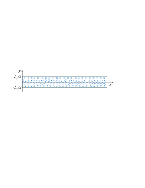
Figure 1: (Color online) A typical view of a highly-ordered ground-state ($\Psi_{n_{l}}=0.96$) colloidal distribution in a channel, for the total density $\rho=0.6\sigma_{col}^{-2}$.

Another essential feature of the colloidal distribution in a channel consists in oscillating dependence of the defect concentration on the channel width $L_{y}$ Doyle . Thus increase of the channel width is periodically accompanied by a qualitative rearrangement of the colloidal structure, namely, by the occurrence of new chains. The values of the channel width, for which the colloidal structures rearrange, correspond to low-ordered states ($\Psi_{n_{l}}\ll 1$) when the stripe structure is hardly distinguishable. This fact is reflected in the oscillation of the stripe order parameter $\Psi_{n_{l}}$ with increasing width of the channel. It is worth to note however that the fact that $\Psi_{n_{l}}$ is large does not mean that the defect concentration is low. Actually it means only that stripes are well pronounced and all defects are mainly topological.

III.2 The integral of motion

Before discussing results of our numerical calculations, we note a useful property that directly follows from system of equations (2), namely, the integral of motion:

$$\eta\sum_{i}\frac{d\vec{r}_{i}}{dt}=\sum_{i}\vec{F}_{dr}(y_{i}).$$ (6)

Separating the longitudinal component we obtain, in terms of average stripe velocities,

$$\eta\sum_{n}\bar{\upsilon}_{xn}=\sum_{n}F_{dr}(y_{n}),$$ (7)

where $n$ denotes the $n$th chain, $\bar{\upsilon}_{xn}$ is the average velocity of $n$th stripe. This expression has a clear meaning: the sum of all average chain velocities is defined by the momentum of the external force transferred to the system. From Eq. (7) it follows that the colloidal system is in the static state, i.e., does not move, only in case of: (i) zero driving force; (ii) sign-alternating driving force satisfying the condition $\sum_{n}F_{dr}(y_{n})=0$ and $max\mid F_{dr}(y_{n})\mid<F_{c}$, where $F_{c}$ is some critical force.

This result is remarkable due to the fact that it differs from the case of particles moving under the action of an external force in any stationary periodic potential. In the latter case, for a commensurate configuration (i.e., when the number of colloids per unit length coincides with the number of potential minima), there is always a threshold value of the force related to the “static friction”. Thus the system of particles moves if the driving force exceeds the threshold value. In our case, the system of colloids moves always when the sum of forces in (7) is larger than zero.

Note that the conservation law (7) is fulfilled for any distribution of the driving force $F_{dr}(y)$ and it is not valid if temperature is non zero.

III.3 Stripe velocity versus non-uniform driving force

In this subsection, we study a response of the colloidal system confined in a channel to an external non-uniform driving force. Clearly, this case is more general than the earlier studied case of a uniform driving created, e.g., by the gravity in inclined channels Leiderer . A gradient driving force produces a shear stress that allows us to examine elastic properties of the colloid “lattice” and to reveal the onset of plastic motion. The transition from elastic to plastic motion leads to a number of different dynamical regimes.

Without loss of generality, we consider two typical profiles of the non-uniform distributed driving force: (i) a linear distributed force given by

$$F_{dr}(y)=F_{max}\left(\frac{1}{2}+\frac{y}{L_{y}}\right),$$ (8)

and (ii) a parabolic distributed driving

$$F_{dr}(y)=F_{max}\left(1-\left(\frac{2y}{L_{y}}\right)^{2}\right),$$ (9)

where $F_{max}=mg\rm{sin}(\alpha)$ is the maximum value of the driving force which we express, for convenience, via the projection of the gravity force that acts on a free colloidal particle being on an inclined plane at angle $\alpha$; $m$ is the mass of the colloidal particle for the density of colloids $\rho_{col}=1600\ kg/m^{3}$ Leiderer .

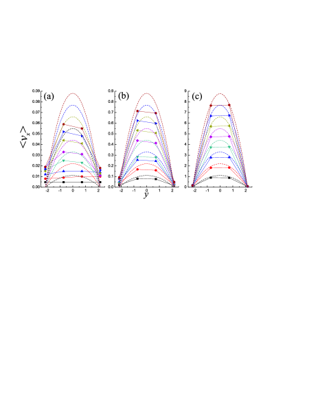
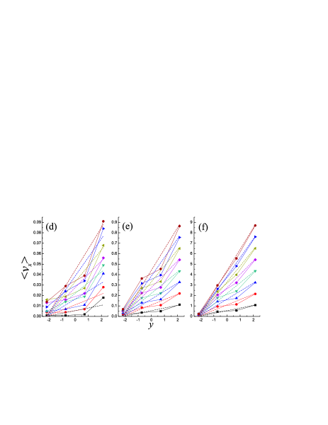
Figure 2: (Color online) The profile of average chain velocities $\langle\upsilon_{x}\rangle$ as a function of the transverse coordinate $y$ for a parabolic ((a) to (c)) and a linear ((d) to (f)) profiles of the applied driving force for various values of $\alpha$: $\alpha=0.01$ to 0.08 ((a), (d)), $\alpha=0.1$ to 0.8 ((b), (e)), and $\alpha=1$ to 8 ((c), (f)). The width of the channel is $L_{y}/\sigma_{col}=4.3$ and the total colloidal density is $\rho=0.6\ \sigma_{col}^{-2}$. The symbols connected by solid lines are average velocities of chains while dashed lines show velocities of (non-interacting) chains corresponding to the distribution of the applied force.

The average velocity of different chains $\bar{\upsilon}_{x}$ as a function of their transverse coordinate $y_{n}$ is presented in Fig. 2 for values of $\alpha$ varying in the range $0.01\leq\alpha\leq 8$. The profiles of the calculated average stripe velocity $\bar{\upsilon}_{x}(y_{n})$ are shown by different symbols (corresponding to different values of driving force expressed in terms of angle $\alpha$, – see the figure captions) connected by solid lines. For comparison, the profiles of stripe velocities in the absence of interaction between the stripes (i.e., renormalized applied external force $F_{dr}(y)/\eta$) are shown by dashed lines, for different magnitudes of the driving force. With increasing $\alpha$ and, accordingly, the total amplitude $F_{max}$ of the driving force the role of the shape of the distribution of applied force on $\bar{\upsilon}_{x}(y_{n})$ increases, while the influence of the structure of colloids and the density of individual chains, $\rho_{chain}(y)$, on the contrary, decreases. In the limit of very large driving force $F_{dr}$ ($1\lesssim\alpha\leq 8$), the distribution of stripe velocity is completely defined by the profile of the applied force $F_{dr}(y)$, as one can expect in the plastic limit (see Figs. 2(c),(f), for parabolic and linear-gradient driving, correspondingly). On the contrary, for small amplitudes $F_{max}$ of the driving force ($0.01\leq\alpha\lesssim 0.05$), deviations of $\bar{\upsilon}_{xn}$ from the profile of the driving force $F_{dr}(y)$ are essential (Fig. 2(a),(d)). This limit corresponds to the elastic or quasi-elastic regime. In the intermediate region of $F_{dr}(y)$, $0.05\lesssim\alpha\lesssim 1$, the function $\bar{\upsilon}_{x}(y_{n})$ is essentially influenced by both factors, $F_{dr}(y)$ and $\rho_{chain}(y)$.

The above behavior is rather general and is typical, in principle, for any profile of the external driving. At the same time, the shape of the driving-force profile is important, especially, in the region of intermediate driving forces. In other words, for the same set of parameters (i.e., the total density, $\rho$, the channel width, $L_{y}$, and $\alpha$) the difference between $F_{dr}$ and $\bar{\upsilon}_{x}$ varies for parabolic and linear profiles of the external driving force.

In order to introduce a measure of conformity of the profiles of the calculated average velocity $\bar{\upsilon}_{x}(y)$ and the external force $F_{dr}$, we define a normalized standard deviation $\Delta$ in the form:

$$\Delta=\sqrt{\sum_{chain}\left(\frac{F_{dr}(y_{chain})/\eta-v_{chain}}{F_{max}}\right)^{2}}.$$ (10)

Low values of $\Delta$ correspond to small difference between $\bar{\upsilon}_{xn}(y)$ and $F_{dr}(y)$. For a parabolic driving-force profile, the gradient of the applied force and thus the shear stress between inner chains is much less than between those at the periphery, while for a linear profile the gradient is constant.

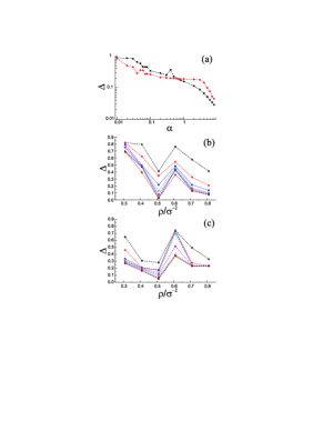
Figure 3: (Color online) The normalized standard deviation $\Delta$ as a function of $\alpha$, calculated from data presented in Fig. 2 (i.e., for a four-chain structure calculated for $\rho=0.6\ \sigma_{col}^{-2}$). Squares (connected by a dot-dashed line) correspond to a linear profile of the driving force; circles correspond to a parabolic profile (a). The function $\Delta$ vs. the total colloidal density $\rho$ for: a parabolic driving force (b) and a linear-gradient driving force (c), for different values of $\alpha=0.1$ to 0.8 (i.e., for three- and four-chain structures as shown in Figs. 4 and 5). Here we use the same symbols as in Fig. 2 to denote velocities of different colloidal stripes.

The results of our calculation of the standard deviation $\Delta$ are shown in Fig. 3 versus driving force (a) and density (b,c), for linear and parabolic profiles of the driving force.

Note that for small driving forces, i.e., for elastic motion, the deviation of the velocity profile $\bar{\upsilon}_{xn}(y)$ from that of the applied driving $F_{dr}(y)$ is less in case of a linear driving-force profile. This means that the elastic deformation of the colloidal “solid” related to a linear driving is stronger than that for a parabolic driving. Contrary, for overall large driving (i.e., $\alpha$), linear-gradient-driven stripes follow the profile of the driving force to a lesser extent than in case of parabolic driving (see Fig. 3(a)). This means that the average dynamical friction between chains is larger in case of a linear-driving applied force. This conclusion seems to be quite surprising keeping in mind the large gradient of the driving force (experienced by peripheral chains) in case of a parabolic driving. As we show below, it can be understood in terms of incommensurability between peripheral chains (i.e., there the driving gradient is maximum) related to different densities of colloids in different chains. The function $\Delta(\rho)$ versus the overall colloidal density is presented in Figs. 3(b) and 3(c), respectively, for parabolic and linear-gradient driving, for different $\alpha$, and $L_{y}/\sigma_{col}=4.3$. Note that in both cases $\Delta(\rho)$ has a minimum at about $\rho=0.5\sigma_{col}^{-2}$ corresponding to a perfect chained structure and incommensurate number of colloids in different chains. As a result, the chains easily slide with respect to each other, and the velocity profile reproduces that of the driving force (if the driving is strong enough, see Figs. 3(b) and (c)). The minimum in $\Delta(\rho)$ at $\rho=0.5\sigma_{col}^{-2}$ is followed by a sharp increase of $\Delta(\rho)$ at about $\rho=0.6\sigma_{col}^{-2}$ explained by the appearance of defects in the chained structure. The defects lock the motion of different chains, similarly to the case of low densities (i.e., $\rho\sim 0.3\sigma_{col}^{-2}$), and the system displays a rigid-body(RB)-like motion. With increasing $\rho$, the maximum in $\Delta$ alternates with a gradual decrease indicating increasing ordering of colloids in stripes. Note that the behavior of $\Delta$ is in general similar for the linear and parabolic driving force (i.e., for high densities $\rho$), the absolute values and dispersion of $\Delta$ for different $\alpha$ are lower in case of the linear-gradient driving, in agreement with the result shown in Fig. 3(a).

III.4 The role of colloidal density in stripes

In order to study the influence of two competing factors, the structural factor $\rho_{chain}(y)$ (i.e., the transverse colloidal density) and the distribution of the external force $F_{dr}(y)$, we performed simulations of colloidal motion for various values of the total density $\rho$ in the intermediate range of values of $\alpha$, $0.1\leq\alpha\leq 0.8$. The average stripe velocity $\bar{\upsilon}_{x}$ as a function of the transverse coordinate $y$ at various values of $\alpha$ and different total colloidal density $\rho$ is presented in Figs. 4 and  5, respectively, for parabolic and linear-gradient profiles of the external force $F_{dr}(y)$. The corresponding distributions of the (normalized) cross-section chain density $\rho_{chain}(y)$ are shown in the bottom panels of Fig. 4.

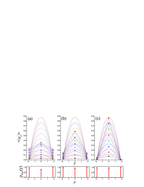
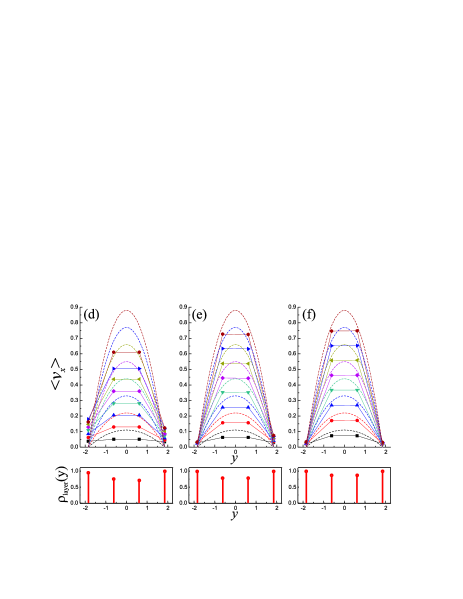
Figure 4: (Color online) Top panels: The profile of average chain velocities $\langle\upsilon_{x}\rangle$ as a function of the transverse coordinate $y$ for a parabolic profile of the applied driving force for various values of $\alpha$ ($\alpha=0.1$ to 0.8) and for the relative width of the channel $L_{y}/\sigma_{col}=3.7$. Bottom panels: The corresponding distributions of the chain densities $\rho_{chain}(y)$ shown for comparison (i.e., normalized on $\rho_{max}$, where $\rho_{max}$ is the maximum density of the chain in the colloidal $n_{l}$-chain configuration). The results are shown for the total density $\rho$: $\rho=0.31\sigma_{col}^{-2}$ (a), $\rho=0.41\sigma_{col}^{-2}$ (a), $\rho=0.51\sigma_{col}^{-2}$ (c), $\rho=0.61\sigma_{col}^{-2}$ (d), $\rho=0.71\sigma_{col}^{-2}$ (e), and $\rho=0.81\sigma_{col}^{-2}$ (f). As in Fig. 2, symbols connected by solid lines show average velocities of chains, and dashed lines show velocities of (non-interacting) chains.

As seen from Fig. 4(a), for the density $\rho=0.31\sigma_{col}^{-2}$ and $\alpha<0.3$ the colloidal structure consists of three stripes and moves as a whole (RB motion). If the colloidal distribution is symmetric with respect to the channel axis $y=0$ then the critical value $\alpha$ of the RB-to-plastic motion increases up to $0.5$. Such an increase of the critical value of $\alpha$ is explained by the simultaneous locking of motion of the central stripe by two adjacent stripes. The transition from the $RB$ mode to the plastic mode occurs only for high enough magnitudes of $F_{max}$ when colloids of the central stripe are capable to overcome the potential barriers created by peripheral stripes. However, in case of an asymmetric (with respect to the channel axis $y=0$) distribution $\rho_{chain}(y)$, the motion of the central stripe is assisted by defects. The potential-energy profile asymmetry, together with the transverse degree of freedom, leads to such type of motion of the central stripe when it avoids obstacles and moves along the potential-energy minimum lines, i.e., along serpentine-like trajectories. This kind of motion provides a lower, as compared to the symmetric case, critical value of $\alpha$ of the transition from RB to plastic mode.

For density $\rho=0.41$, the RB mode is observed only for the lowest value $\alpha=0.1$ (Fig. 4(b)). For larger densities the RB mode of motion is not observed in the range of $\alpha=$0.1 to 0.8 (Fig. 4(c)-(f)) but it can be realized for even smaller values of $\alpha$. Note, however, that for $\rho=0.61\sigma_{col}^{-2}$ (Fig. 4(d)) (the least dense state of a four-chain phase) at $\alpha=0.1$ the motion almost corresponds to the RB mode.

Comparison of the cases of a parabolic (Fig. 4) and a linear (Fig. 5) driving forces clearly shows the difference in the conditions of the manifestation of the RB mode. In particular, for a linear-gradient force $F_{dr}(y)$ this mode is observed for values $\alpha\leq 0.1$ and total density $\rho=0.31\sigma_{col}^{-2}$ (i.e., the lowest-$\rho$ three-chain phase), that means a lower threshold magnitude $F_{max}$ of the transition from elastic to plastic mode of colloidal motion (cp. Figs. 4(a) and 5(a)). At the same time, for the lowest-$\rho$ four-chain phase, this threshold value is higher $(\alpha\leq 0.4)$ in case of a linear driving than for a parabolic, as can be seen from Figs. 4(d) and  5(d). This means that the RB mode manifests itself for: (i) a parabolic driving force $F_{dr}(y)$ in the case of the lowest-$\rho$ three-chain phase and (ii) a linear $F_{dr}(y)$ in case of the lowest-$\rho$ four-chain phase.

The observed behavior is explained as follows. In case of a parabolic driving of the lowest-$\rho$ three-chain structure, the driving is applied to the central stripe. The motion of this stripe is locked by the potential created by two adjacent stripes. The most stable is a symmetric configuration, i.e., when two peripheral stripes are mirror-symmetric with respect to the axis of the channel $y=0$, and thus the potential created by them is double the potential created by a single stripe. Thus, the symmetric configuration favors the RB mode. For asymmetric configurations, the RB-to-plastic mode threshold is lower. In this case the motion of the central stripe (i.e., for driving higher than a critical value) is serpentine-like, i.e., the central stripe deforms in the $y$-direction following the minimum potential-energy path. A typical dispersion of the trajectory of the central stripe in the transverse direction is $\Delta y\approx 0.1$ (while $\Delta y\approx 10^{-4}$ to $10^{-3}$ for the symmetric case). As a result, the lowest-$\rho$ three-chain colloidal structure is characterized by a relatively high threshold of the RB-to-plastic transition, under a parabolic-profile driving (see Fig. 4(a)). In case of a linear-gradient driving of the lowest-$\rho$ three-chain phase (Fig. 5(a)), the maximum driving force is applied to one of the peripheral chains. In the RB mode, its motion is locked only by the adjacent central chain. When unlocked, the peripheral chain also provides an additional driving applied to the central chain. The central chain adjusts itself to follow the minimum potential-energy path between the two peripheral chains. This motion is characterized by a rather large transverse dispersion, $\Delta y\approx 0.2$ to $0.3$, that facilitates an easy sliding of the three chains with respect to each other.

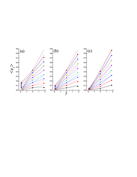
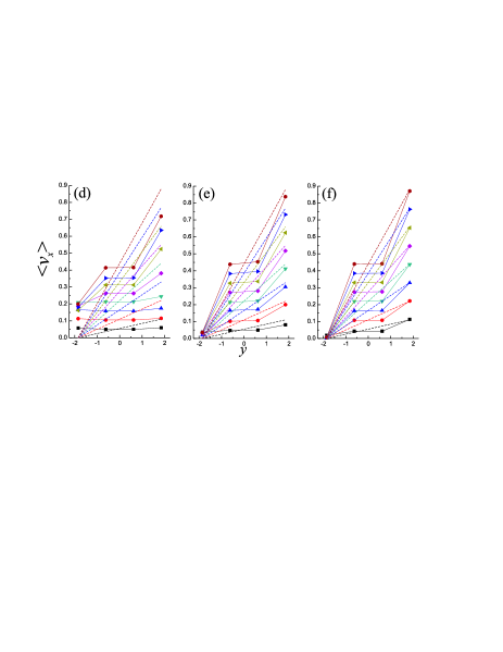
Figure 5: (Color online) The profile of average chain velocities $\langle\upsilon_{x}\rangle$ as a function of the transverse coordinate $y$ for a liner-gradient profile of the applied driving force for various values of $\alpha$ ($\alpha=$0.1 to 0.8) and for relative width of the channel $L_{y}/\sigma_{col}=3.7$. The results are shown for the total density $\rho$: $\rho=0.31\sigma_{col}^{-2}$ (a), $\rho=0.41\sigma_{col}^{-2}$ (a), $\rho=0.51\sigma_{col}^{-2}$ (c), $\rho=0.61\sigma_{col}^{-2}$ (d), $\rho=0.71\sigma_{col}^{-2}$ (e), and $\rho=0.81\sigma_{col}^{-2}$ (f). As in Fig. 2, symbols connected by solid lines show average velocities of chains, and dashed lines show velocities of (non-interacting) chains.

The situation is quite different in case of the lowest-$\rho$ four-layer phase shown in Figs. 4(d) and  5(d). In the ground-state low-$\rho$ four-chain configurations, two central chains have lower density than the peripheral chains (see bottom panels in Figs. 5(d), (e), and (f)). Thus, the potential profile created by the central chains is deeper, and they survive a rather strong shear stress (similar to the case of low-density 1D chains in a harmonic potential in the Frenkel-Kontorova model BraunKivshar ). Such shear stress is negligible for a parabolic driving (it appears as a result of transverse instabilities). Thus the central part of the four-chain structure remain in the RB mode for very large values of driving, and it also does in case of a linear-gradient driving (see Figs. 4(d), (e), and (f)). However, the higher-$\rho$ peripheral chains produce shallower potential-energy profiles, and thus the friction between them and the central chains is weak BraunKivshar . It is clear than that in case of a parabolic driving the peripheral stripes can easily slide with respect to the central stripes, and thus the RB-to-plastic mode threshold is rather low (Fig. 4(d)). In contrast, a relatively weak (i.e., for the same $F_{max}$) gradient of the driving force in case of a linear-gradient driving provides a high threshold of the RB-to-plastic mode transition (Fig. 5(d)).

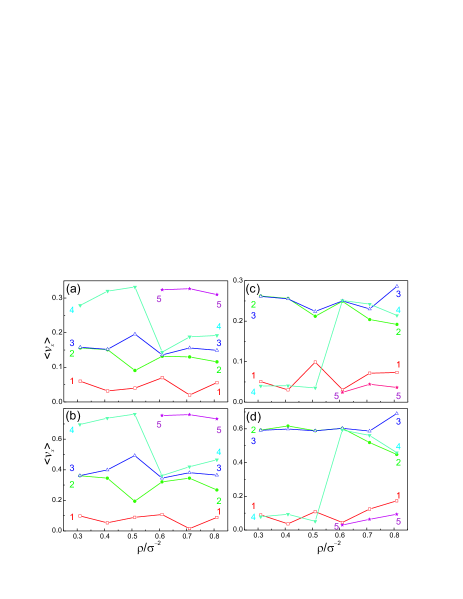
Figure 6: (Color online) Average stripe velocities $\langle\upsilon_{x}\rangle$ as a function of the total colloidal density $\rho$ for a linear ((a), (b)) and a parabolic ((c), (d)) profiles of the applied driving force, for the channel width $L_{y}/\sigma_{col}=5$, and for different driving: $\alpha=0.3$ ((a), (c)) and $\alpha=0.7$ ((b), (d)). Different symbols connected by solid lines show $\langle\upsilon_{x}\rangle$ of different chains marked for clarity by numbers 1, 2, 3, 4, and 5 (the numbers are shown by the same color as the corresponding curves).

As we discussed above, the colloidal distribution in a channel depends on the width of the channel and the total colloidal density. For certain “matching” sets of these parameters, colloids form well-defined stripe structures characterized by a maximum value of the order parameter $\Psi_{n_{l}}=1$, while small values of the order parameter $\Psi_{n_{l}}\ll 1$ correspond to non-chained structure. It is interesting then to follow the evolution of stripe velocities when changing the total colloidal density in the channel stripes . The results of calculations are presented in Fig. 6 for a linear-gradient ((a), (b)) and a parabolic ((c), (d)) profile of the driving force and different magnitudes of driving. Let us consider first the case of a linear driving. At low density, $\rho=0.3\sigma_{col}^{-2}$, the colloids form four stripes (marked by numbers 1, 2, 3, and 4 of the same color as the corresponding lines/symbols), and for all values of $\alpha$ (i.e., $\alpha=0.3$ (a) and 0.7 (b)) shown in Fig. 6, two central chains (2 and 3) turn out to be locked while the peripheral chains (1 and 4) (which have a higher stripe density $\rho_{chain}$ and are incommensurate with the central chains) slide with respect to the central chains. With increasing $\rho$, e.g., $\rho=0.4\sigma_{col}^{-2}$ for $\alpha=0.7$ (see Fig. 6(b)) the central chains 2 and 3 unlock. This is explained by decreasing of the inter-colloid distance in stripes and thus by shallowing of the potential profile created by them. Note that for a weaker driving $\alpha=0.3$ (a), the central stripes remain locked at $\rho=0.4\sigma_{col}^{-2}$ and they unlock at a higher value of $\rho$: $\rho=0.5\sigma_{col}^{-2}$. For even higher density, $\rho=0.6\sigma_{col}^{-2}$, the inter-shell defects lock the motion of the central chains 2 and 3 (and partially of all the chains), and the whole stripe structure collapses. If we still increase the colloid density, a new stripe (5) originates from the “disordered” phase, and for larger $\rho$ (i.e., $\rho=0.8\sigma_{col}^{-2}$) the motion of all five stripes unlock, and they move with individual velocities. Note that the transition of the system from the state with $n_{l}$ stripes to the state with $n_{l}+1$ stripes occurs always through the disordered phase (i.e., when all or some of the stripes lose their identity, and colloids of these “stripes” move with the same velocity as, e.g., stripes 2, 3, and 4 in Fig. 6(a) and (b) at $\rho=0.6\sigma_{col}^{-2}$). Thus the disordered phase of the motion serves as a “bifurcation point” that gives rise to a new state with $n_{l}+1$ velocity branches. The evolution of stripe velocities for a parabolic driving occurs in a similar way (Fig. 6(c) and (d)), although the degenerate velocities of the central stripes, 2 and 3 (and those of the peripheral stripes, 1 and 4, which are separated from the velocities of the central stripes by a wide gap), unlock only for rather high density.

It is also interesting to note an oscillating behavior of the velocity of motion of the peripheral stripes driven only by the interaction with adjacent stripes. The oscillation in velocity reflects the oscillation of the friction force between the stripes with increasing total colloidal density.

IV Mobility of stripes and dynamical phases of their motion

As shown above, the response of the system of colloidal stripes (i.e., the profile of individual velocities of different stripes) to the external non-uniform driving is, in general, nonlinear: the velocity profile of the stripes is not scalable with the driving (i.e., for all values of the driving, although there are regions of scalability which will be discussed below).

In order to systematically examine the response of the colloidal system to an external driving, we analyze the mobility of different chains under the action of a delta-like driving force applied to one of the chains:

$$F_{dr}(y)=F_{drk}(y)=F_{max}\delta(y-y_{k,i}),$$ (11)

where $\delta(y-y_{k,i})=1$, if $y=y_{k,i}$, and $\delta(y-y_{k,i})=0$, if $y\neq y_{k,i}$, $y_{k,i}$ is the coordinate of $i$th particle of $k$th stripe driving and $F_{max}$ is the driving force as defined in Eq. (9). We simulated the colloidal motion in a channel of width $L_{y}/\sigma_{col}=4$ for various colloidal densities $\rho$. For such a channel and considered densities $\rho$, the ground state of the system corresponds to a three-stripe structure characterized by a high value of the order parameter $\Psi_{3}\approx 1$. Fig. 7 shows the results of calculation for the mobilities versus driving force $F_{drk}$ for different stripes $B_{n,k}=\bar{\upsilon}_{xn}/F_{drk}$, where $\bar{\upsilon}_{xn}$ is the average velocity of $n$th stripe, and $F_{drk}$ is the force applied to $k$th stripe. (Here we show only the case when driving is applied to one peripheral stripe. Applying driving to other stripes results in a similar behavior.) Note that the mobility is defined by $B_{k,k}=\bar{\upsilon}_{xk}/F_{drk}$, while $B_{n,k}$ for $k\neq n$ is a mobile response of the stripes.

As seen from Fig. 7, the mobility as a function of the applied force exhibits a variety of modes of motion. First, we stress the most general features of the behavior. A stripe mobility $B_{k,k}$ tends to unity in the limit of large applied force $F_{drk}$, and mobile responses $B_{n,k}$, correspondingly, vanish, as seen from Fig. 7. This limit corresponds to the plastic mode of motion. Another general conclusion refers to the RB-to-plastic transition: this transition shifts towards lower drivings with increasing the total colloidal density (cp. Figs. 7(a) and (b)). As we discussed above, a growth of the colloidal density results in a hardening of the rigidity of the elastic stripes BraunKivshar and a simultaneous weakening of the inter-stripe friction.

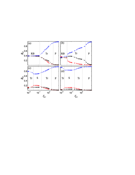
Figure 7: (Color online) The mobility $B_{k,k}$ and mobile response $B_{n,k}(n\neq k)$ of different stripes as a function of driving force applied to $k$th stripe ($k=1$) at various values of the total density: $\rho=0.45\sigma_{col}^{-2}$ (a), $\rho=0.55\sigma_{col}^{-2}$ (b), $\rho=0.65\sigma_{col}^{-2}$ (c), and $\rho=0.75\sigma_{col}^{-2}$ (d). The mobility (mobile response) of different stripes are shown by different symbols: $B_{1,1}$ ($\Box$), $B_{1,2}$ ($\bigcirc$), and $B_{1,3}$ ($\triangle$).

However, apart from these general features, the mobilities display other important peculiarities. To discuss these, let us define dynamical phases corresponding to different regimes of colloidal motion in channels. We denote the first regime as “RB” (“rigid body”, or elastic motion). This regime is most pronounced for low colloidal density, $\rho=0.45\sigma_{col}^{-2}$ (Fig. 7(a)), where it extends to $F_{dr1}\approx 1.05$. For $\rho=0.55\sigma_{col}^{-2}$ (Fig. 7(b)) the threshold value reduced by a factor of five, $F_{dr1}\approx 0.2$. For higher densities, the RB-to-plastic mode transition shifts towards very low values of $F_{dr1}$. The RB regime is followed by a broad transition region (“Tr”) characterized by a monotonic increase of the mobility $B_{k,k}$ (and monotonic decrease of the mobile responses $B_{n,k}$). While this growth is close to linear in Fig. 7(a), for higher density it displays oscillations in Fig. 7(b). Remarkably, for higher colloidal densities these oscillations turn to regions of decreasing colloid mobility $B_{k,k}$ versus driving force. Note that this regime (denoted as “S”) is similar to the dynamically-ordered phase of vortex motion in superconductors with arrays of regular pinning sites dynphfn ; dynphwe . This ordered phase follows a disordered phase with a higher density of average vortex flow and thus leads to the appearance of a negative differential resistivity (NDR) part of N-type in the VI-curve dynphwe . In our case of colloidal motion in a narrow channel, we observe a similar effect characterized by a slowing down of the motion of the stripe driven by an external force (with a simultaneous increase of the velocity of the adjacent stripes) when increasing the applied driving force. In this region, the system of colloids displays a partial “reentrant” behavior (cp. Refs. dzubiellajpcm ; dzubiellapre ) when, being melted by increasing shear stress, it starts evolving towards a solid phase with further increasing driving. Note that this dynamically-induced “solidification” has common features with the recently discovered transition “freezing by heating” fbhprl ; fbhnat where by increasing temperature it leads to the crystallization of moving repulsive interacting particles which are in a molten state.

The mechanism of the observed colloid solidification can be understood as follows. As we discussed above, the longitudinal motion of colloidal stripes is accompanied by transverse oscillations of the stripes’ trajectories (i.e., serpentine-like motion) related to the asymmetry of the potential-energy profiles created by the adjacent stripes. For low drivings (but larger than the critical driving force of the RB-to-plastic transition), the stripe driven by an external force moves along some serpentine-like trajectory. When moving, the stripe itself deforms adjusting to the potential-energy landscape. In its turn, it elastically deforms other stripes due to the interaction with colloids in the adjacent stripes. At low velocities, colloids in adjacent stripes relax to the initial state thus providing low friction between the stripes. Increasing the velocity of motion of the driven stripe (at high colloid density) leads to increasing rate of the inter-stripe collisions and to the development of instabilities in the transverse direction. This results in an increase of the dynamical friction between stripes which explains the observed decrease of the mobility $B_{k,k}$ (and increase of the mobile response $B_{n,k}$), i.e., the appearance of “S” phase. Very large driving, however, straightens the trajectories of motion of the driven stripe. In the limit of $F_{dr}\to\infty$, the driven stripe moves along unrelaxed in the $y$-direction straight trajectory, and the mobility $B_{k,k}\to 1$ (while the mobile response $B_{n,k}\to 0$), as shown in Figs. 7(c), (d).

V Conclusions

We have studied the dynamics of colloids driven by an external non-uniform force in a narrow channel. We focused on colloidal densities which provide well-defined colloidal stripe structures. In the limit of a very low driving force the system moves as a rigid body (elastic motion) independent of the profile of the driving force. In the opposite limit of a very strong driving force, the profile of the average velocities of colloidal stripes follow the profile of the applied driving (plastic regime). While these limiting-case results are easily understandable, the dynamics of colloidal stripes in the general case is rather complex. It is governed by the interplay of several factors, i.e.: (i) the magnitude and profile of driving force; (ii) the total density of the colloidal system and the distribution of the colloidal density in stripes, and, as a consequence, (iii) commensurability effects between the adjacent chains. We have shown that depending on the density and number of stripes, the transition from elastic to plastic motion occurs at different values of the driving force. For example, the lowest-density three-stripe colloidal configuration is shown to be more robust with respect to a parabolic driving than to a linear-gradient driving, while for the lowest-density four-stripe configuration the situation is opposite. This result is explained by the colloidal density distribution over the central (lower density) and the peripheral (higher density) stripes and commensurability effects. We have analyzed the mobility of colloidal stripes and have identified the dynamical phases of their motion. In particular, it has been shown that the transition from elastic (rigid-body-motion phase) to plastic mode, depending on the density of colloids, could be either monotonic (i.e., characterized by a gradual increase of the mobility), or it could contain an NDR-type part (i.e., characterized by a drop of mobility versus driving force). This unusual “solidification” is related to the dynamically-induced increase of the friction in the colloidal system and is similar to the recently discovered “freezing by heating” transition. The results of our study, with corresponding changes, can also be applied to other systems of interacting particles driven by a non-uniform force in narrow channels, e.g., in physics or biology.

VI Acknowledgments

This work was supported by the “Odysseus” program of the Flemish Government and Flemish Science Foundation (FWO-Vl). V.R.M. acknowledges the support by the EU Marie Curie project, Contract No. MIF1-CT-2006-040816.

References

- (1) K. Mangold, P. Leiderer, and C. Bechinger, Phys. Rev. Lett. 90, 158302 (2003).
- (2) Y. Han, N.Y. Ha, A.M. Alsayed, and A.G. Yodh, Phys. Rev. E 77, 041406 (2008).
- (3) F. Bürzle and P. Nielaba, Phys. Rev. E 76, 051112 (2007).
- (4) A. Libál, C. Reichhardt, and C.J. Olson Reichhardt, Phys. Rev. E 78, 031401 (2008).
- (5) C.V. Achim, M. Karttunen, K.R. Elder, E. Granato, T. Ala-Nissila, and S.C. Ying, Phys. Rev. E 74, 021104 (2006).
- (6) R. Haghgooie, P.S. Doyle, Phys. Rev. E 70, 061408 (2004).
- (7) A. Ricci, P. Nielaba, S. Sengupta, and K. Binder, Phys. Rev. E 74, 010404(R) (2006).
- (8) T.R. Stratton, S. Novikov, R. Qato, S. Villarreal, B. Cui, S.A. Rice, and B. Lin, Phys. Rev. E 79, 031406 (2009).
- (9) M. Köppl, P. Henseler, A. Erbe, P. Nielaba, and P. Leiderer, Phys. Rev. Lett. 97, 208302 (2006).
- (10) P. Henseler, C.A. Erbe, M. Köppl, P. Leiderer, and P. Nielaba, arXiv:0810.2302v1 [cond-mat.soft] 13 Oct 2008.
- (11) G. Piacente and F.M. Peeters, Phys. Rev. B 72, 205208 (2005).
- (12) G. Piacente, I.V. Schweigert, J.J. Betouras, and F.M. Peeters, Phys. Rev. B 69, 045324 (2004).
- (13) V. Nosenko, J. Goree, Z.W. Ma, and A. Piel, Phys. Rev. Lett. 88, 135001 (2002).
- (14) K. Jiang, L.-J. Hou, Y.-N. Wang, and Z.L. Mikovi, Phys. Rev. E 73, 016404 (2006).
- (15) M. Wolter and A. Melzer, Phys. Rev. E 71, 036414 (2005).
- (16) A. Libál, C. Reichhardt, and C.J. Olson Reichhardt, Phys. Rev. Lett. 97, 228302 (2006).
- (17) V. Misko, S. Savel’ev, and F. Nori, Phys. Rev. Lett. 95, 177007 (2005).
- (18) I.V. Grigorieva, W. Escoffier, V.R. Misko, B.J. Baelus, F.M. Peeters, L.Y. Vinnikov, and S. Dubonos, Phys. Rev. Lett. 99, 147003 (2007).
- (19) N.S. Lin, V.R. Misko, and F. Peeters, Phys. Rev. Lett. 102, 197003 (2009).
- (20) Q.-H. Wei, C. Bechinger, and P. Leiderer, Science 287, 625 (2000).
- (21) M. Kollmann, Phys. Rev. Lett. 90, 180602 (2003).
- (22) A. Taloni and F. Marchesoni, Phys. Rev. Lett. 96, 020601 2006.
- (23) G. Coupier, M. Saint Jean, and C. Guthmann, Phys. Rev. E 73, 031112 (2006).
- (24) K. Nelissen, V.R. Misko, and F.M. Peeters, Europhys. Lett. 80, 56004 (2007).
- (25) O.M. Braun and Y.S. Kivshar, The Frenkel-Kontorova model. Concepts, methods and applications. Springer (2004).
- (26) Note that although stripes are not well defined for low values of the order parameter , we still call them “stripes”. We start from well-defined (i.e., narrow) chains and then follow the evolution of the stripes even though they broaden.
- (27) This means that the driving force is applied to all the particles of th stripe, even if their individual transverse coordinates deviate from the average -coordinate of the stripe.
- (28) C. Reichhardt, C.J. Olson, and F. Nori, Phys. Rev. Lett. 78, 2648 (1997); Phys. Rev. B 58, 6534 (1998).
- (29) V.R. Misko, S. Savel’ev, A.L. Rakhmanov, and F. Nori, Phys. Rev. Lett. 96, 127004 (2006); Phys. Rev. B 75, 024509 (2007).
- (30) J. Dzubiella and H. Lowen, J. Phys.: Condens. Matter 14, 9383 (2002).
- (31) J. Chakrabarti, J. Dzubiella, and H. Lowen, Phys. Rev. E 68, 061407 (2004).
- (32) D. Helbing, I.J. Farkas, and T. Vicsek, Phys. Rev. Lett. 84, 1240 (2000).
- (33) H.E. Stanley, Nature (London) 404, 718 (2000).