Lyapunov exponent and natural invariant density determination of chaotic maps: An iterative maximum entropy ansatz

Abstract

We apply the maximum entropy principle to construct the natural invariant density and Lyapunov exponent of one-dimensional chaotic maps. Using a novel function reconstruction technique that is based on the solution of Hausdorff moment problem via maximizing Shannon entropy, we estimate the invariant density and the Lyapunov exponent of nonlinear maps in one-dimension from a knowledge of finite number of moments. The accuracy and the stability of the algorithm are illustrated by comparing our results to a number of nonlinear maps for which the exact analytical results are available. Furthermore, we also consider a very complex example for which no exact analytical result for invariant density is available. A comparison of our results to those available in the literature is also discussed.

1 Introduction

The classical moment problem (CMP) is an archetypal example of an inverse problem that involves reconstruction of a non-negative density distribution from a knowledge of (usually finite) moments [1, 2, 3, 4, 5, 6]. The CMP is an important inverse problem that has attracted researchers from many diverse fields of science and engineering ranging from geological prospecting, computer tomography, medical imaging to transport in complex inhomogeneous media [7]. Much of the early developments in the fields such as continued fractions and orthogonal polynomials have been inspired by this problem [2, 8]. The extent to which an unknown density function can be determined depends on the amount of information available in the form of moments provided that the underlying moment problem is solvable. For a finite number of moments, it is not possible to obtain the unique solution and one needs to supplement additional information to construct a suitable solution. The maximum entropy provides a suitable framework to reconstruct a least biased solution by simultaneously maximizing the entropy and satisfying the constraints defined by the moments [9].

In this communication we address how the maximum entropy (ME) principle can be applied to the Hausdorff moment problem [1] in order to estimate the Lyapunov exponent and the associated natural invariant density of a nonlinear dynamical system. In particular, we wish to apply our ME ansatz to a number of nonlinear iterative maps in one-dimension for which the analytical results in the closed form are available. The problem was studied by Steeb et al [10] via entropy optimization for the tent and the logistic maps using the first few moments (up to 3). Recently, Ding and Mead [11, 12] addressed the problem and applied their maximum entropy algorithm based on power moments to compute the Lyapunov exponents for a number of chaotic maps. The authors generated Lyapunov exponents using up to the first 12 moments, and obtained an accuracy of the order of 1%. In this paper, we address the problem using a method based on an iterative construction of maximum entropy solution of the moment problem, and apply it to compute Lyapunov exponents and the natural invariant densities for a number of one-dimensional chaotic maps. Unlike the power moment problem that becomes ill-conditioned with the increasing number of moments, the hallmark of our method is to construct a stable algorithm by resort to moments of Chebyshev polynomials. The resulting algorithm is found to be very stable and accurate, and is capable of generating Lyapunov exponents with an error less than 1 part in $10^{3}$, which is significantly lower than any of the methods reported earlier [10, 11]. Furthermore, the method can reproduce the natural invariant density of the chaotic maps that shows point-wise convergence to the exact density function whenever available.

The rest of the paper is organized as follows. In Section 2, we briefly introduce the Hausdorff moment problem and a discrete maximum entropy ansatz to construct the least biased solution that satisfies the moment constraints. This is followed by Section 3, where we introduce the natural invariant density as an eigenfunction of the Perron-Frobenius operator associated with the dynamical system represented by the iterative maps [13]. In Section 4, we discuss how the moments of the invariant density are computed numerically via time evolution of the dynamical variable, which are then used to construct the Lyapunov exponents and the natural invariant densities of the maps. Finally, in Section 5, we discuss the results of our method and compare our approximated results to the exact results and to those available in the literature.

2 Maximum Entropy approach to the Hausdorff moment problem

The classical moment problem for a finite interval [a, b], also known as the Hausdorff moment problem, can be stated loosely as follows. Consider a set of moments

$$\mu_{i}=\int_{a}^{b}x^{i}\,\rho(x)\,dx\quad\quad i=0,1,2,\ldots,m,\quad i\leq m$$ (1)

of a function $\rho(x)$ integrable over the interval with $\mu_{i}<\infty$ $\forall\,x\in$ [a,b] and $\rho(x)$ has bounded variation, the problem is to construct the non-negative function $\rho(x)$ from a knowledge of the moments. The necessary and sufficient conditions for a solution to exist were given by Hausdorff [1]. The moment problem and its variants have been discussed extensively in the literature [2, 3, 14, 15] at length, and an authoritative treatment of the problem with applications to many physical systems was given by Mead and Papanicolaou [4]. For a finite number of moments, the problem is underdetermined and it is not possible to construct the unique solution from the moment sequence unless further assumptions about the function are made. Within the maximum entropy framework, one attempts to find a density $\rho_{A}(x)$ that maximizes the information entropy functional,

$$S[\rho]=-\int_{a}^{b}\rho_{A}(x)\,\ln[\rho_{A}(x)]\,dx$$ (2)

subject to the moment constraints defined by Eq. (1). The resulting solution is an approximate density function $\rho_{A}(x)$ and can be written as

$$\rho_{A}(x)=\exp\left(-\sum_{i=0}^{m}\lambda_{i}\,x^{i}\right).$$ (3)

The normalized density function $\rho(x)$ is often referred to as probability density by mapping the interval to [0,1] without any loss of generality. For a normalized density with $\mu_{0}$ = 1, the Lagrange multiplier $\lambda_{0}$ is connected to the others via

$$e^{\lambda_{0}} = \int_{0}^{1}\exp\left(-\sum_{i=1}^{m}\lambda_{i}x^{i}\right)$$

A reliable scheme to match the moments numerically for the entropy optimization problem (EOP) was discussed by one of us in Ref. [16]. The essential idea behind the approach was to use a discretized form of entropy functional and the moment constraints using an accurate quadrature with a view to reduce the original constraint optimization problem in primal variables to an unconstrained convex optimization program involving dual variables. This guarantees the existence of the unique solution [17], which is least biased and satisfies the moment constraints defined by Eq. (1). Using a suitable quadrature, the discretized entropy and the moment constraints can be expressed as respectively,

$$S[\rho] = -\int_{0}^{1}\rho(x)\,\ln[\rho(x)]\,dx\,\approx\,-\sum_{j=1}^{n}\omega_{j}\,\rho_{j}\,\ln\rho_{j}$$ (4)

$$\mu_{i} = \int_{0}^{1}x^{i}\,\rho(x)\,dx\,\approx\,\sum_{j=1}^{n}\,(x_{j})^{i}\,\omega_{j}\,\rho_{j}$$ (5)

where $\omega_{i}$’s are a set of weights associated with the quadrature and $\rho_{j}$ is the value of the distribution at $x=x_{j}$. If $\omega_{j}$ and $x_{j}$ are the weight and abscissas of the Gaussian-Legendre quadrature, the Eq. (4) is exact for polynomials of order up to $2\,n-1$, and

$$\sum_{j=1}^{n}\omega_{j}=1,\qquad\qquad\sum_{j=1}^{n}\omega_{j}\,\rho_{j}=1.$$ (6)

The task of our EOP can now be stated as, using $\tilde{\rho}_{j}=\omega_{j}\rho_{j}$ and $t_{ij}=(x_{j})^{i}$, to optimize the Lagrangian

$$L(\tilde{\rho},{\bf\tilde{\lambda}})=\sum_{j=1}^{n}\tilde{\rho}_{j}\,\ln\left(\frac{\tilde{\rho}_{j}}{\omega_{j}}\right)-\sum_{i=1}^{m}\tilde{\lambda}_{i}\left(\sum_{j=1}^{n}t_{ij}\,\tilde{\rho}_{j}-\mu_{i}\right)$$ (7)

where $0\leq\tilde{\rho}\in R^{n}$ and $\tilde{\lambda}\in R^{m}$, respectively are the primal and dual variables of the EOP, and the discrete solution is given by functional variation with respect to the unknown density,

$$\tilde{\rho}_{j}=\omega_{j}\exp\left(\sum_{i=1}^{m}t_{ij}\,\tilde{\lambda}_{i}-1\right),\quad j=1,2,\ldots n.$$ (8)

The Eqs. (4) to (8) can be combined together and a set of nonlinear equations can be constructed to solve for the Lagrange multipliers $\tilde{\lambda}$

$$F_{i}({\bf\tilde{\lambda}})=\sum_{j=1}^{n}t_{ij}\,\omega_{j}\,\exp\left(\sum_{k=1}^{m}t_{kj}\,\tilde{\lambda}_{k}-1\right)-\mu_{i}=0,\quad i=1,2,\ldots,m.$$

The set of nonlinear equations above can be reduced to an unconstrained convex optimization problem involving the dual variables:

$$\min_{\tilde{\lambda}\in R^{m}}\left[D(\tilde{\lambda})\equiv\sum_{j=1}^{n}\tilde{\rho}_{j}\,\exp\left(\sum_{i=1}^{m}t_{ij}\,\tilde{\lambda}_{i}-1\right)-\sum_{i=1}^{m}\mu_{i}\,\tilde{\lambda}_{i}\right].$$ (9)

By iteratively obtaining an estimate of $\tilde{\lambda}$, $D({\tilde{\lambda}})$ can be minimized, and the EOP solution ${\rho}(\tilde{\lambda}^{*})$ can be constructed from Eq. (8). In the equation above, $t_{ij}=x_{j}^{i}$ corresponds to power moments, but the algorithm can be implemented using Chebyshev polynomials as well. The details of the implementation of the above approach for shifted Chebyshev polynomials was discussed in Ref [16]. The maximum entropy solution in this case is still given by the Eq.(3) except that $x^{i}$ within the exponential term is now replaced by $T^{*}_{i}(x)$, where $T^{*}_{i}(x)$ is the shifted Chebyshev polynomials. In the following, we apply the algorithm based on the shifted Chebyshev moments to construct the invariant density of the maps.

3 Lyapunov exponent and the natural invariant density of chaotic maps

The Lyapunov exponent of an ergodic map can be expressed in terms of the natural invariant density of the map:

$$\Gamma=\int\rho(x)\,\ln|f^{\prime}(x)|\,dx$$ (10)

where $\rho(x)$ is the invariant density and $f^{\prime}(x)$ is the first derivative of the map $f(x)$ with respect to the dynamical variable $x$. The invariant density of a map can be defined as an eigenfunction of Perron-Frobenius operator associated with the map. Given an iterative map, $x_{n+1}$ = $f(x_{n})$, one can construct an ensemble of initial iterates $\{x_{0}\}$ defined by a density function $\rho_{0}(x)$ in some subspace of the phase space and consider the time evolution of the density in the phase space instead of initial iterates $x_{0}$. The corresponding evolution operator $L$ is known as Perron-Frobenius operator, which is linear in nature as each member of the ensemble in the subspace evolves independently. The invariant density can be written as,

$$L\,\rho(x)=\rho(x)$$ (11)

where $\rho(x)$ is a fixed point of the operator $L$ in the function space. In general, there may exist multiple fixed points but only one has a distinct physical meaning, which is referred to as the natural invariant density. Following Beck and Schlögl [13], the general form of the operator in one-dimension can be written as,

$$L\,\rho(y)=\sum_{x\in f^{-1}(y)}\frac{\rho(x)}{|f^{\prime}(x)|}.$$ (12)

For an one-dimensional map, one can define the Lyapunov exponent as the exponential rate of divergence of two arbitrarily close initial points separated by $\delta x_{n=0}=|x_{0}-x^{\prime}_{0}|$ in the limit $n\to\infty$, and the exponent can be expressed as the average of the time series of the iterative map,

$$\Gamma=\frac{1}{N}\lim_{N\to\infty}\sum^{N-1}_{n=0}\ln|f^{\prime}(x_{n})|.$$ (13)

For ergodic maps the time average of the Lyapunov exponent can be replaced by the ensemble average,

$$\Gamma=\int dx\;\rho(x)\;\ln|f^{\prime}(x)|$$ (14)

using the natural invariant density. Equation (14) suggests that the Lyapunov exponent can be obtained from a knowledge of the reconstructed natural invariant density from the moments. In the following we consider some nonlinear maps to illustrate how the normalized invariant density and Lyapunov exponent can be calculated using our discrete entropy optimization procedure.

4 Reconstruction of invariant density as a maximum entropy problem

In the preceding sections, we have discussed how a probability density can be constructed from a knowledge of the moments (of the density) by maximizing the information entropy along with the moment constraints. Once the density is reconstructed, the Lyapunov exponent can calculated from Eq. (14) using the reconstructed density. The calculation of the moments can proceed as follows. We consider a dynamical system represented by a nonlinear one-dimensional map,

$$x_{n+1}=f(x_{n})\\$$

where $n$=0, 1, 2, …and $x_{0}\in[0,1]$. The power moment of the time evolution of the iterate $x_{n}$ can be expressed as,

$$<x^{i}>=\lim_{t\to\infty}\frac{1}{t}\sum_{n=0}^{t}(x_{n})^{i}$$

Since we are working with the shifted Chebyshev polynomials, the corresponding moments are,

$$\mu_{i}=\lim_{t\to\infty}\frac{1}{t}\sum_{n=0}^{t}{T_{i}}^{*}(x_{n})$$ (15)

where $T_{i}^{*}(x)$ are the shifted Chebyshev polynomials and are related to Chebyshev polynomials via $T_{i}^{*}(x)=T_{i}(2\,x-1)$, and $x\in[0,1]$. A set of shifted Chebyshev moments can be constructed numerically from Eq. (15), which can be used to obtain an approximate natural invariant density as discussed earlier. This approximate density can then be used to calculate Lyapunov exponents for the maps via Eq. (14). By varying the number of moments, the convergence of the approximated invariant density function can be systematically studied and the accuracy of the Lyapunov exponent can be improved. We first apply our method to the maps for which the exact analytical results are available. Thereafter, we consider a nontrivial case where neither the Lyapunov exponent, nor the density can be obtained analytically and consists of a series of sharp peaks with fine structure which is difficult to represent using the form of analytical expression proposed by the maximum entropy solution.

5 Results and Discussions

Let us first consider the case for which the invariant density function and the Lyapunov exponent can be calculated analytically. We begin with the map,

$$f_{1}(x)=\left\{\begin{array}[]{ll}\frac{2x}{1-x^{2}}&\mbox{$0\leq x\leq\sqrt{2}-1$}\\ \\ \frac{1-x^{2}}{2x}&\mbox{$\sqrt{2}-1\leq x\leq 1$}\end{array}\right.$$ (16)

The invariant density for this map can be written as

$$\rho_{1}(x)=\frac{4}{\pi(1+x^{2})}$$ (17)

and the Lyapunov exponent is given by $\ln 2$, which can be obtained analytically from Eq. (14).

Table 1: Test Map $f_{1}$

Moments	$\Gamma_{\mathrm{maxent}}$	Percentage error
20	0.691577	0.226
40	0.692786	0.055
60	0.692999	0.021
80	0.693061	0.012
100	0.693109	0.006
$\Gamma_{\mathrm{exact}}$	$\ln 2\approx$ 0.693147
$\Gamma_{\mbox{{\scriptsize Ref.~{}\cite[cite]{[\@@bibref{}{Ding1}{}{}]}}}}$	0.69290

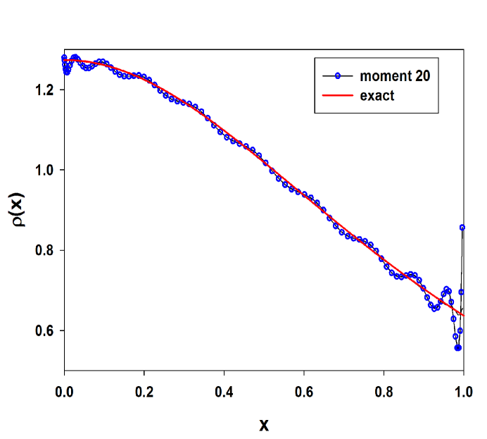
Figure 1: The reconstructed density from the first 20 Chebyshev moments for the map $f_{1}(x)$ along with the exact density. Although the general shape of the density appears correctly, some oscillations are present in the data in absence of sufficient information.

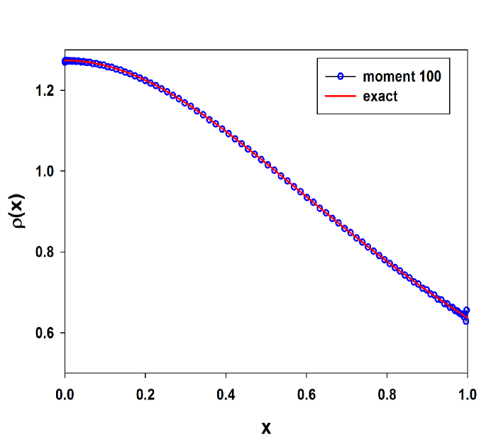
Figure 2: The reconstructed density obtained from the first 100 moments for the map $f_{1}(x)$ along with the exact density. The approximate density now effectively matches point-by-point with the exact one with the exception of few points near the edges of the interval.

The approximated Chebyshev moments for the map $f_{1}(x)$ can be obtained numerically from Eq. (15). The ME ansatz is then applied to reconstruct the invariant density, and the Lyapunov exponent is obtained from this estimated invariant density. The results for the Lyapunov exponent are summarized in table 1 for different set of moments. The data clearly indicate that the approximated Lyapunov exponent rapidly converges to the exact value $\ln 2\approx$ 0.693147 with the increase of number of moments. The error associated with the exponent is also tabulated, which shows that for the case of 100 moments the percentage error is as small as 0.006 reflecting the accurate and the stable nature of the algorithm. In order to verify our method further, we now compare the approximated density to the exact density given by Eq. (17). This is particularly important because integrated quantities (such as Lyapunov exponent) are, in general, less sensitive to any approximation then the integrand (invariant density) itself, and that often makes it possible to get an accurate value of Lyapunov exponent from a reasonably correct density. In figs.1 and 2, we have plotted the approximated densities for two different set of moments along with the exact density. Since the density is smooth and free from any fine structure, only the first 20 moments are found to be sufficient to get the correct shape of the density although some oscillations are present in the reconstructed density. On increasing the number of moments, the oscillations begin to disappear and for 100 moments the approximate density matches very closely with the exact one. The reconstructed density is shown in fig.2, and it is evident from the figure that the density practically matches point-by-point with the exact density.

As a further test of our method, we now consider the case of logistic map. The map played a very important role in the development of the theory of nonlinear dynamical systems [18], and can display a rather complex behavior depending on the control parameter $r$ defined via,

$$f_{2}(x)=r\;x\,(1-x).$$ (18)

We consider three representative values of $r$ to illustrate our method in the chaotic and non-chaotic domain. In particular, we choose (a) $r=\frac{5}{2}$, (b) $r$=4, and (c) $r$ = 3.79285. The analytical densities are known only for the first two cases, and are given by respectively,

$$\rho_{2}^{\mathrm{chaotic}}(x)=\frac{1}{\pi\sqrt{x-x^{2}}};\quad\quad\,\,r=4\\$$ (19)

$$\rho_{2}^{\mathrm{fixed}}(x)=\delta\left(x-\frac{3}{5}\right);\quad\quad r=\frac{5}{2}$$ (20)

For the remaining value of $r=3.79285$, no analytical expression for the density is known and the density consists of a number of sharp peaks along with some fine structure. The density in this case can be obtained numerically by iterating a set of initial $x_{0}$, and constructing a histogram averaging over a number of configurations [13]. For the purpose of comparison to our maximum entropy results, we use this numerical density here.

Table 2: Logistic Map: Case A $f_{2}=\frac{5}{2}x\,(1-x)$

Moments	$\Gamma_{\mathrm{maxent}}$	Percentage error
10	$-$0.693575	0.063
20	$-$0.693851	0.101
30	$-$0.693203	0.008
40	$-$0.693155	0.002
$\Gamma_{\mathrm{exact}}$	$-\ln 2\approx$ $-0.693147$

Table 3: Logistic Map: Case B $f_{2}=4\,x\,(1-x)$

Moments	$\Gamma_{\mathrm{maxent}}$	Percentage error
40	0.690703	0.35
60	0.692101	0.15
80	0.692850	0.04
100	0.693319	0.02
$\Gamma_{\mathrm{exact}}$	$\ln 2$ $\approx$ 0.693147
$\Gamma_{\mbox{{\scriptsize Ref.~{}\cite[cite]{[\@@bibref{}{Ding1}{}{}]}}}}$	0.68425

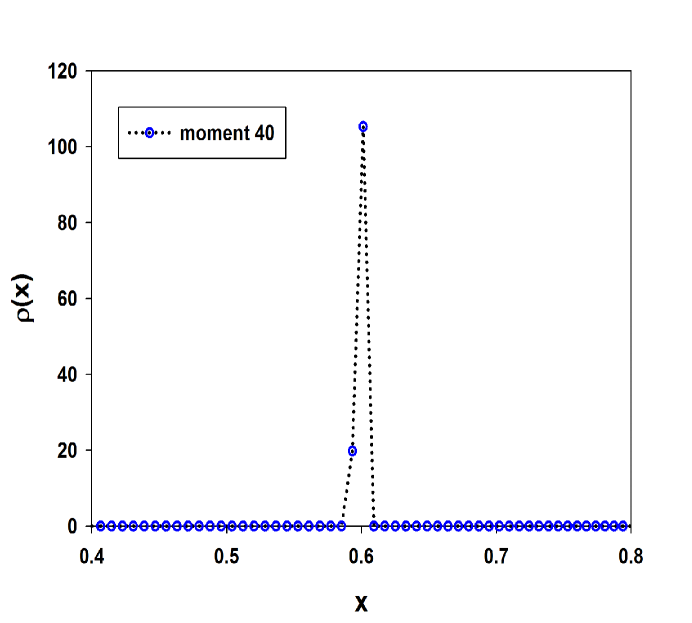
Figure 3: The reconstructed density for the logistic map for $r=\frac{5}{2}$ obtained from the first 40 Chebyshev moments. The density consists of only two non-zero values in the interval [0.593, 0.601]. The exact density is a $\delta$-function centered at $x_{0}=\frac{3}{5}$.

In tables 2 and 3 we have listed the values of the Lyapunov exponents for different number of moments for $r=\frac{5}{2}$ and $r=4$ respectively. The errors associated with $\Gamma$ are also listed in the respective tables. The invariant density for $r=\frac{5}{2}$ is a $\delta$-function, and the exact analytical value of the exponent is given by $-\ln 2$. Since the invariant density is a $\delta$-function at $x_{0}=\frac{3}{5}$, it is practically impossible to reproduce the density very accurately using a finite number of quadrature points. However, our maximum entropy algorithm produces an impressive result by generating only two non-zero values in the interval containing the point $x_{0}=\frac{3}{5}$ using Gaussian quadrature with 192 points. The approximate density for a set of 40 moments is shown in fig. 3. The two non-zero values of the density are given by 19.781 and 105.264 within the interval [0.593, 0.601]. It may be noted that for a normalized density, one can estimate the maximum height of the $\delta$-function to be of the order of $({\Delta x})^{-1}\approx 125.0$, where $\Delta x$ is the interval containing the point $x_{0}=\frac{3}{5}$ point [19]. Furthermore, we have found that the result is almost independent of the number of moments (beyond the first 20), and the $\delta$-function has been observed to be correctly reproduced with few non-zero values using only as few as first 10 moments. Table 3 clearly shows that the first 3 digits have been correctly reproduced using only the first 10 moments. On increasing the number of moments, there is but very little improvement of the accuracy of Lyapunov exponent. For each of the moment sets, the density is found to be zero throughout the interval except at few (two for the set 40 and higher) points mentioned above. In absence of any structure in the density, higher moments do not contribute much to the density reconstruction, and hence it’s more or less independent of the number of moments. Since the contribution to the Lyapunov exponent is coming only from the few (mostly two) non-zero values, and that these values fluctuate with varying moments, an oscillation of these values causes a mild oscillation in the Lyapunov exponent.

We now consider the case $r=4$. The exact density in this case is given by Eq. (19) that has singularities at the end points $x$ = 0 and 1. It is therefore instructive to study the divergence behavior of the reconstructed density near the end points. In fig.4 we have plotted the approximate density obtained using the first 90 moments along with the exact density. The reconstructed density matches excellently within the interval. The divergence behavior near $x=0$ is also plotted in the inset. Although there is some deviation from the exact density, the approximate density matches very good except at very small values of $x$. Such observation is also found to be true near $x=1$. The results for the Lyapunov exponent are listed in table 3 for different number of moments. It is remarkable that the exponent has been correctly produced up to 3 decimal points with 100 moments. While the error in this case is larger compared to the cases discussed before for the same number of moments, it is much smaller than the result reported earlier [11]. Our numerical investigation suggests that the integral converges slowly for Gaussian quadrature in this case owing to the presence of a logarithmic singularity in the integrand. This requires one to use more Gaussian points to evaluate the integral correctly. However, since the density itself has singularities at the end points, attempts to construct the density very close to the end points introduce error in the reconstructed density that affects the integral value. The use of Gauss-Chebyshev quadrature would ameliorate the latter problem, but for the purpose of generality (and in absence of prior knowledge of the density) we refrain ourselves from using the Gauss-Chebyshev quadrature.

Finally, we consider a case where analytical results are not available and the density consists of several sharp peaks having fine structure in the interval [0,1]. As mentioned earlier, the case $r=3.79285$ for the logistic map provides such an example. The ‘exact’ numerical density for this case is shown in fig. 5 along with the reconstructed density for 20 moments. The former is obtained by iterating several starting $x_{0}$ and constructing an histogram of the distribution of the iterates in the long time limit, which is then finally averaged over many configurations. While our MEP ansatz produces most of the peaks in the exact density using the first 20 moments, the fine structure of the peaks is missing and so is the location of the peaks. The reconstructed density can be improved systematically by increasing the number of moments, and for 150 moments the density matches very good with the exact density. In fig. 6 we have plotted both the reconstructed density for the first 150 moments and the numerical density from the histogram method. The result suggests that for sufficient number of moments our algorithm is capable of reproducing density which is highly irregular, non-differentiable and consists of several sharp peaks.

6 Conclusion

We apply an iterative maximum entropy optimization technique based on Chebyshev moments to calculate the invariant density and the Lyapunov exponent for a number of one-dimensional nonlinear maps. The method consists of evaluating approximate moments of the invariant density from the time evolution of the dynamical variable of the iterative map, and to apply a novel function reconstruction technique via maximum entropy optimization subject to moment constraints. The computed Lyapunov exponents from the approximated natural invariant density are found to be in excellent agreement with the exact analytical values. We demonstrate that the accuracy of the Lyapunov exponent can be systematically improved by increasing the number of moments used in the (density) reconstruction process. An important aspect of our method is that it is very stable and accurate, and that it does not require the use of extended precision arithmetic for solving the moment problem. A comparison to the results obtained from power moments suggest that the algorithm based on Chebyshev polynomials gives more accurate results than the power moments. This can be explained by taking into account the superior minimax property of the Chebyshev polynomials and the form of the maximum entropy solution for Chebyshev moments [20, 21]. Our method is particularly suitable for maps for which exact analytical expression for invariant density are not available. Since the method can deal with a large number of moments, an accurate invariant density function can be constructed by studying the convergence behavior with respect to the number of moments. The Lyapunov exponent can be obtained from a knowledge of the invariant density of the maps. Finally, the method can also be adapted to solve non-linear differential and integral equations as discussed in Refs.[22] and [23], which we will address in a future communication.

PB acknowledges the partial support from the Aubrey Keith Lucas and Ella Ginn Lucas Endowment in the form of a fellowship under faculty excellence in research program. He also thanks Professor Arun K. Bhattacharya of the University of Burdwan (India) for several comments and discussions during the course of the work.

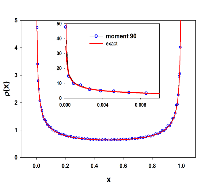
Figure 4: The reconstructed density for the map $f_{2}(x)$ for $r=4$ obtained from the first 90 moments along with the exact density. The density matches excellently within the interval. The divergence behavior at the left edge near $x=0$ is also shown in the inset.

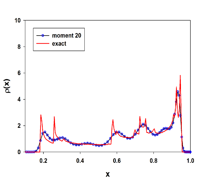
Figure 5: The reconstructed density for the logistic map for $r=3.7928$ from the first 20 Chebyshev moments along with the ‘exact’ numerical density obtained via histogram method and averaged over 5000 configurations. While our maximum entropy algorithm produces most of peaks in the density, the fine structure of the peaks is missing in absence of information coming from the higher order moments.

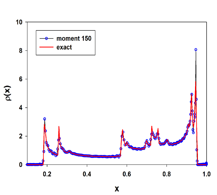
Figure 6: The reconstructed density for logistic map for $r=3.7928$ obtained from the first 150 Chebyshev moments. The corresponding ‘exact’ density obtained from the map averaged over 5000 configurations is also plotted for comparison. The height and the position of the peaks are now correctly reproduced using the first 150 moments.

References

- [1] Hausdorff F, Math Z. 16, 220-248 (1923)
- [2] Shohat J A and Tamarkin J D, The Problem of Moments (American Mathematical Society, Providence, RI, 1963)
- [3] Akheizer, N. I,The classical moment problem and some related questions in analysis, Hafner Publishing Co., New York 1965
- [4] Mead, L.R. and Papanicolaou, N. J. Math. Phys. 25, 8 (1984)
- [5] A. Tagliani, J. Math. Phys. 34, 326 (1993)
- [6] R.V. Abramov, J. of Computational Physics, 226, 621 (2007)
- [7] Kirsch, A. An Introduction to Mathematical Theory of Inverse Problems, Springer-Verlag, New York
- [8] R. Haydock in Solid State Physics: Advances in Research and Applications, Vol 35 edited F.Seitz, Academic Press (1980)
- [9] Jaynes E. T, Probability Theory: The Logic of Science (Cambridge University Press, Cambridge, U. K., 2003)
- [10] Steeb W-H, Solms F and Stoop R 1994 J. Phys. A: Math. Gen. 27 L399
- [11] Ding J and Mead L R 2002 J. of Math. Phys. 43 2518
- [12] J. Ding and L.R. Mead, Appl. Math. & Comp. 185, 658 (2007)
- [13] Beck, C and Schlögl, F Thermodynamics of chaotic systems (Cambridge University Press, Cambridge, MA, 1993)
- [14] Wimp, J., Proc. Roy. Soc. Edinburgh 82 A, 273 (1989)
- [15] M. Junk, Math. Models Methods Appl. Sci 10, 1001 (2000)
- [16] Bandyopadhyay K, Bhattacharya A K, Biswas P and Drabold D A 2005 Phys. Rev. E 71 057701
- [17] The solution is unique in the sense that it is least biased as far as entropy of the density is concerned, and the Hausdorff conditions are satisfied. There is no guarantee that the maximum entropy solution would be close to the exact solution particularly for very few moments. However, the quality of the MEP solution drastically improves with increasing number of moments, and numerical experiments for cases where exact solutions are known confirm that maximum entropy principle indeed can produce the correct solution.
- [18] Feigenbaum, M.J. J. Stat. Phys. 19, 25 (1978); May, R.M. Nature 261, 459 (1976)
- [19] For a sufficiently small interval, can be approximated by a box function of width around and of height , giving = 1 to satisfy the normalization condition. The height of the -function obtained in our work is very close to this limiting value.
- [20] The presence of in the maximum entropy solution for power moments makes it very difficult to exploit information from the high order moments for in the interval [0, 1] even with extended precision arithmetic. Such a problem does not appear in our formulation of the problem via Chebyshev moments owing to the bounded nature of Chebyshev polynomials, and consequently provides a way to incorporate systematically the information from the higher moments.
- [21] Mason, J.C and Handscomb, D.C Chebyshev Polynomials (Chapman and Hall/CRC, New York, USA 2003)
- [22] J. Baker-Jarvis and D. Schultz, Numerical Methods for Partial Differential Equations, 5, 133-142 (1989), John Wiley & Sons Inc,
- [23] L.R. Mead, J. Math. Phys. 27, December 1986