Flow-level models for multipath routing

Abstract

In this paper we study coordinated multipath routing at the flow-level in networks with routes of length one. As a first step the static case is considered, in which the number of flows is fixed. A clustering pattern in the rate allocation is identified, and we describe a finite algorithm to find this rate allocation and the clustering explicitly. Then we consider the dynamic model, in which there are stochastic arrivals and departures; we do so for models with both streaming and elastic traffic, and where a peak-rate is imposed on the elastic flows (to be thought of as an access rate). Lacking explicit expressions for the equilibrium distribution of the Markov process under consideration, we study its fluid and diffusion limits; in particular, we prove uniqueness of the equilibrium point. We demonstrate through a specific example how the diffusion limit can be identified; it also reveals structural results about the clustering pattern when the minimal rate is very small and the network grows large.

1 Introduction

Balancing flows over different routes, commonly referred to as multipath routing, bears important advantages. First, it makes the network more robust, because in case of a link failure, the flow can still use bandwidth on its other routes. Also, under multipath routing the resources of the network are used more efficiently since overcongested flows have more flexibility to spread their traffic over undercongested parts of the network. In this paper we want to elaborate on the latter aspect. Questions we are particularly interested in are: How are the resources shared under multipath routing, what causes congestion, and how are these congestion phenomena affected by the number of routes that a flow can use?

Recently, multipath routing has attracted substantial attention from the research community. We specifically mention here models that consider the flow-level, i.e., the timescale at which the number of flows stochastically changes: flows arrive at the network, use a set of links for a while, and then leave. Flows can be divided into streaming and elastic flows: streaming flows (voice, real-time video) are essentially characterized by their duration and the rate they transmit at; on the other hand, elastic flows (predominantly data) are characterized by their size, while their transmission rate is a function of the level of congestion in the network. An implicit assumption in flow-level models is that of separation of time-scales, meaning that the time it takes for the rate to adapt is negligible compared to changes at the flow-level. A flow-level model for multipath routing, which integrates elastic and streaming traffic, is due to Key and Massoulié [7]; models in the context of rate control can be found in the work by Kelly and Voice [5, 13].

In this paper we consider multipath routing at the flow-level in networks with routes of length one, adopting the model of [7] for coordinated multipath routing. Here coordinated multipath routing means that rates are allocated so as to maximize the utilities of the total rates that flows obtain. This is in contrast with uncoordinated multipath routing, where flows on different routes are treated as different users; then one maximizes the utilities of the rates that a flow achieves on each route. As pointed out in [7], such an uncoordinated mechanism generally leads to inferior performance. There a fluid limit for the model of integrated streaming and elastic traffic was established, and uniqueness of the equilibrium point was proven. A first contribution of our work is that we consider a perhaps more realistic model in which the elastic flows have an upper bound they can transmit at. Imposing such a peak rate has significant advantages when analyzing the model [1]; in addition it has a natural interpretation, as the constraint on the rate can be thought of as the rate of the bottleneck link (for instance the access rate). For this model we establish a fluid limit, and prove existence and uniqueness of an equilibrium point; in addition we describe a (finite) algorithm that finds this equilibrium point.

One of the difficulties in the analysis of multipath routing, is that the rate allocation cannot be given explicitly, even when the number of flows is fixed; instead, it follows by solving an optimization problem. Additionally, this optimization problem contains further variables, determining how users split their flow on different routes, for which there is in general no unique solution. The second contribution of this paper, is that we ease this analysis by finding generalized cut constraints for the case of routes of length one. These generalized cut constraints assume there are certain cuts, i.e., subsets of resources, of the network that give sufficient constraints to determine the feasibility of a flow. Introducing these reduces the optimization problem to one with the total rates being the only variables over which we are optimizing. In the rate allocation for a given number of flows, we identify a clustering of flows and resources. The generalized cut constraints enable us to construct an algorithm that finds the rate allocation and the clustering explicitly.

Related to the question how flows share resources in a multipath network, a crucial concept is complete resource pooling, which is a state in which the network behaves as if all resources are pooled together, with every user having access to it. It is clearly desirable to achieve this state, as then resources can be shared fairly among all flows and, due to the concavity of the utility functions we are using, in the most utility-efficient way. (Also, this implies that if a network is already in complete resource pooling then increasing the number of routes that a flow can use does not change the rate allocation since the network already operates in the best possible way. However, increasing the number of routes will make it more likely for the network to be in a complete resource pooling state.) Complete resource pooling was already studied by, e.g., Laws [9] and Turner [11] for networks where users must use one route only but have a set of possible routes to choose from. In this paper, we give explicit conditions for the equilibrium point of the fluid limit to be of the complete-resource-pooling type.

Our last contribution relates to the purely symmetric circle network. Each flow is allowed to use $r$ given routes; we call the network a circle network as the resources can be arranged in a circle. This setup is reminiscent of the supermarket model by Mitzenmacher [10], where every flow chooses one of a set of $r$ randomly chosen routes; we believe our model is the more natural one, as users would naturally choose from a set of routes in their proximity. We study the effect increasing $r$, the number of routes that a flow can use, has on congestion in the network. To this end we define ‘congestion’ as the event that there is a flow that can transmit at a rate of at most some small value $\epsilon$. We then investigate in what kind of cluster this congestion event is most likely to occur. Using diffusion-based estimates, we derive expressions for the corresponding probabilities, and conclude that, as the size of the network grows large, the cluster with highest probability of congestion has size $r-1$.

The outline of the paper is as follows. In Section 2 we introduce the model of multipath routing in general networks. We describe the optimization problem that gives the rate allocation for a given number of flows. For the case of routes of length one we describe the clustering in the rate allocation, and introduce notions of connected and strongly connected sets. In this context we also introduce the generalized cut constraints. Section 3 further investigates the rate allocation, for a given number of flows. We develop the algorithm that identifies this allocation, which also gives explicit expressions for the maximum and minimum rate (over all flows), as well as a lower bound on the rate allocated to each of the flows.

In Section 4 we then move to the model that incorporates a flow level, and which involves streaming and (peak-rate constrained) elastic traffic, as described above. In the scenario of streaming traffic only, the stationary distribution of the corresponding Markov chain is given explicitly, but for the other cases this is infeasible. We therefore resort to fluid limits in Section 5. After briefly reviewing the results of [7], we specifically consider the fluid limit for peak-rate constraint elastic traffic, and prove the uniqueness of an equilibrium point. We also introduce the concept of complete resource pooling, and provide conditions for the equilibrium point of the fluid limit to be in complete resource pooling for both cases, with integrated streaming and elastic traffic and with peak-rate constraint elastic traffic.

In Section 6 we turn to the diffusions around the equilibrium point. We explicitly establish the diffusion limit for the purely symmetric circle network. We will calculate the covariance matrix of the stationary distribution that belongs to this diffusion. Relying on these estimates, we present expressions for the probabilities that congestion occurs (that is, some transmission rates are below some critical value $\epsilon$) with a cluster of size $k$, so as to identify the most-likely size of the cluster in periods of congestion.

2 Definitions and preliminaries

In this section we first define in our multipath setting, given the number of flows present, the allocation of rates to these flows. We will make this allocation more explicit in the next section. In practice, of course, the number of flows will change over time; in Section 4 and further we consider this setting (where we use the results derived in Section 3 for a given number of flows present). A second goal of this section is to introduce useful notions such as clusters and (strong) connectivity.

2.1 Rate allocation

We consider networks with multipath routing, i.e., we have a set of resources $J$ with capacities $(C_{j})_{j\in J}$, users (interchangeably referred to as flow types) $I$ and routes $R$. User $i$ can use routes in $R(i)\subseteq R$, where each route $r\in R$ is a set of resources $r\subseteq J$. As mentioned above, in this and the following section we still consider the number of flows to be fixed.

Let $n_{i}$ denote the number of file transfers of type $i$ then the vector $(x_{i})_{i\in I}$ of rates allocated to flow of type $i$ is the unique solution to the concave optimization problem:

$$\begin{array}[]{rrll}\mbox{Maximize}&\quad\sum_{i\in I}{n_{i}U_{i}(x_{i})}&\\ \mbox{s.t.}&\quad\sum_{r:j\in r,i:r\in R(i)}{n_{i}x_{i}^{r}}&\leq C_{j}&\quad\forall j\in J,\\ &\quad\sum_{r\in R(i)}{x_{i}^{r}}&=x_{i}&\quad\forall i\in I,\\ &\quad x_{i}^{r}&\geq 0&\quad\forall i\in I,r\in R(i).\end{array}$$ (1)

Here $x_{i}^{r}$ is the rate with which flow of type $i$ is processed on route $r$. We agree that $x_{i}=0$ if $n_{i}=0$. Also, we can define variables $x_{i}^{r}=0$ for $r\in R(i)$. Following [7], the utility functions $U_{i}$ are assumed to be strictly concave, strictly increasing and differentiable. A utility function that is frequently considered in this context is

$$U_{i}(x)=w_{i}\frac{x^{1-\alpha}}{1-\alpha},$$

for given weights $w_{i}$; this type of utility curves is usually referred to as weighted $\alpha$-fairness. In this paper we will disregard weights and consider $U_{i}(\cdot)=U(\cdot)$, i.e., each user has the same utility function.

Considering routes of length one only, the following results are irrespective of the explicit form of the function U and only require that it is a strictly concave, strictly increasing , and differentiable common utility function. Here we leave the notion of route, and let $J(i)$ be the set of resources user $i$ can use. Now, $x_{i}^{j}$ denotes the rate user $i$ receives from resource $j$. Then our optimization problem reads:

$$\begin{array}[]{rrll}\mbox{Maximize}&\quad\sum_{i\in I}{n_{i}U(x_{i})}&\\ \mbox{s.t.}&\quad\sum_{i:j\in J(i)}{n_{i}x_{i}^{j}}&\leq C_{j}&\quad\forall j\in J,\\ &\quad\sum_{j\in J(i)}{x_{i}^{j}}&=x_{i}&\quad\forall i\in I,\\ &\quad x_{i}^{j}&\geq 0&\quad\forall i\in I,j\in J(i).\end{array}$$ (2)

The stationary conditions of the corresponding Lagrangian are

$$\begin{array}[]{rrll}\forall i,j\in J(i):&x_{i}&\geq(U^{\prime})^{-1}(\mu_{j})&\quad\mbox{with equality if $x_{i}^{j}>0$}\\ &\sum_{i:j\in J(i)}{n_{i}x_{i}^{j}}&=C_{j}&\quad\mbox{$\forall j$ s.t. $\exists i,j\in J(i),n_{i}>0,$}\end{array}$$ (3)

where $\mu_{j}$ is the Lagrange multipliers corresponding to resource $j$. Then we can see that for any function $U$ as above the optimal solution $x$ is sufficiently characterized by

$$\begin{array}[]{rll}x_{i_{1}}>x_{i_{2}}\;\Rightarrow\;x_{i_{1}}^{j}&=0&\quad\forall j\in J(i_{1})\cap J(i_{2})\\ \sum_{i:j\in J(i)}{n_{i}x_{i}^{j}}&=C_{j}&\quad\mbox{$\forall j$ s.t. $\exists i,j\in J(i),n_{i}>0,$}\end{array}$$ (4)

2.2 Clusters, connectivity

With (4) we can discover a unique partition of $(I,J)$ into a collection of clusters of the form $(I^{\prime},J^{\prime})$ , similarly to Hajek’s notion [2]. This is the same for any strictly concave differentiable function $U$.

Definition 2.1.

We define a cluster to be a non-empty pair $(I^{\prime},J^{\prime})$ with $I^{\prime}\subseteq I$, $J^{\prime}\subseteq J$ such that if $i\in I^{\prime}$ then $I^{\prime}$ consists of all $i^{\prime}\in I$ such that there exists a path $i=i_{0},i_{1},i_{2},..i_{n}=i^{\prime}\in I^{\prime},j_{1},j_{2}...j_{n}\in J^{\prime}$ such that for a feasible allocation $x$ solving (2) $x_{i_{k-1}}^{j_{k}}$ and $x_{i_{k}}^{j_{k}}$ are strictly positive for all $k=1,...n$. Similarly, $J^{\prime}$ consists of all $j\in J$ for which there exists a path $i=i_{0},i_{1},i_{2},..i_{n-1}\in I^{\prime},j_{1},j_{2}...j_{n}=j\in J^{\prime}$ such that for a feasible allocation $x$ solving (2) $x_{i_{k-1}}^{j_{k}}$ and $x_{i_{k}}^{j_{k}}$ are strictly positive for all $k=1,...n$. with $x_{i}^{j}>0$

This gives indeed a unique partition since it can be checked that the existence of a path between $i$ and $j$, or respectively between $i$ and $j^{\prime}$ or $j$ and $j^{\prime}$, is an equivalence relation. It can be easily deduced from (4) that if $i$ and $i^{\prime}$ are in the same cluster then $x_{i^{\prime}}=x_{i}$.

Intuitively, a cluster $(I^{\prime},J^{\prime})$ is such that the optimal rate allocation is as if all resources of $J^{\prime}$ are pooled together with exactly all flows of $I^{\prime}$ having access to it. Consider Figure 1 which shows a circle network of four resources (described by squares labelled 1, 2, 3, and 4) of unit capacity and four flow types (described by circles labelled 1, 2, 3, and 4). Each type $i$ can use resources $i$ and $i+1$, which is illustrated by edges (where $4+1$ is understood as 1). In this example $n_{1}$, the number of flows of type 1, is relatively large, ie. suppose $n_{1}=4,n_{2}=n_{3}=n_{4}=1$, so that flows of type 1 monopolize resources 1 and 2. Types 2, 3 and 4 are sharing resources 3 and 4 equally. Thus we have two clusters, one consisting of flows of type 1 and resources 1 and 2, and another consisting of flow types 2, 3, and 4 and resources 3 and 4.

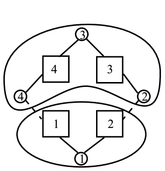
Figure 1: Possible clustering for a circle network with four resources

As a consequence of the previous definition all flows $i$ in the same cluster will have the same rate $x_{i}$. If we have two distinct clusters in which the common rate $x_{i}$ is the same, then we say that these clusters are at the same cluster level.

For a cluster $(I^{\prime},J^{\prime})$ we then have that the set $I(J^{\prime})=\{i\in I:J(i)\subseteq J^{\prime}\}$, i.e., the set consisting of all $i$ that have to go through $J^{\prime}$, is a subset of $I^{\prime}$. We will be particularly interested in the event of complete resource pooling, i.e., when $(I,J)$ is just a single cluster.

The following notions of connectivity help us to characterize the structure of the network and to identify clusters. These notions concern the general structure of $(I,J,J(i))$ without taking into account the allocation at state $n$.

Definition 2.2.

A pair $(I^{\prime},J^{\prime})$ with $I^{\prime}\subseteq I$, $J^{\prime}\subseteq J$ is connected if $J^{\prime}$ cannot be partitioned in nonempty $J_{1},J_{2}$ such that $I^{\prime}$ can be partitioned into $I_{1}$, $I_{2}$ with $J(i)\cap J_{2}=\emptyset$ for $i\in I_{1}$ and $J(i)\cap J_{1}=\emptyset$ for $i\in I_{2}$. Equivalently, for all $j,j^{\prime}\in J^{\prime}$ there is a path $i_{1},i_{2},..i_{n}\in I^{\prime},j_{0}=j,j_{1},j_{2}...j_{n}=j^{\prime}\in J^{\prime}$ such that $j_{k},j_{k+1}\in J(i_{k+1})$ for all $k=0,..n-1$

Regarding $(I,J,J(i))$ as a bipartite graph with nodes $I$ and $J$ and an edge between $i\in I$ and $j\in J$ if and only if $j\in J(i)$, we see that a pair $(I^{\prime},J^{\prime})$ is connected if and only if the subgraph $(I^{\prime},J^{\prime})$ is connected. We can also see that for $(I^{\prime},J^{\prime})$ to be a cluster it has to be connected.

Definition 2.3.

A subset $J^{\prime}\subseteq J$ is connected if $(I,J^{\prime})$ is connected. We define $\mathscr{C}(J)$ to be the set of connected subsets of $J$. A subset $J^{\prime}\subseteq J$ is strongly connected if $(I(J^{\prime}),J^{\prime})$ is connected. Let $\mathscr{SC}(J)$ be the set of strongly connected subsets of $J$.

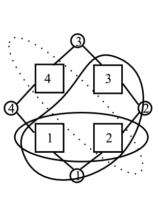
Figure 2: Connected sets of resources in the circle network with four resources

Figure 2 demonstrates connected sets of the circle network with four resources from Figure 1. Any set of consecutive resources $\{1,2\}$, $\{1,2,3\}$ and also $\{1,2,3,4\}$ and $\{1\}$ are connected as are the sets isomorphic to these. Here, all of these sets are also strongly connected since consider eg. $I(\{1,2,3\})=\{2,3\}$ and any splitting of $\{1,2,3\}$ into two non-empty sets would lose either user 2 or 3.

It is immediate that ‘strongly connected’ implies ‘connected’. However, the reverse is not true as Figure 3 illustrates. Here the set of resources 1, 2 and 3 is connected, but not strongly connected, since we can partition it in subsets $\{1,2\}$ and $\{3\}$. Then $I(\{1,2,3\})$, which contains flow type 1 only, is the same as $I(\{1,2\})$. The notion of strongly connected sets is so important because it enables us to identify the generalized cut constraints in the next section, and they are also essential to the rate-allocation algorithm of Section 3.

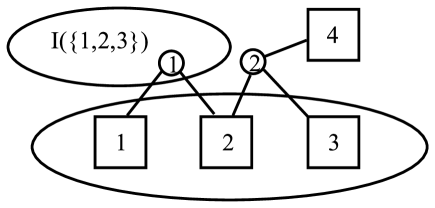
Figure 3: Network with set of resources $\{1,2,3\}$ being connected but not strongly connected

2.3 Generalized cut constraints

The feasibility constraints from (2) are inconvenient because they involve additional variables $x_{i}^{j}$ for which there is no unique solution. However, we can rewrite them in terms of the $x_{i}$ as

$$\sum_{i\in I(J^{\prime})}{n_{i}x_{i}}\leq\sum_{j\in J^{\prime}}{C_{j}}\quad\forall J^{\prime}\in\mathscr{SC}(J).$$ (5)

These inequalities are called generalized cut constraints. They will be inevitable in the next section when proving the validity of the optimal allocation attained by our proposed algorithm. The equivalence of these generalized cut constraints to the feasibility constraints from (2) is proved in Lemma A.1 in the appendix. Kang et al. [6] have shown in their Proposition 5.1 that it is possible even for the general multipath network to write the feasibility constraints in terms of generalized cut constraints as

$$A(nx)\leq C$$

where $A$ is a some non-negative matrix and $C$ is a positive vector; here $(nx)$ refers to the vector with $i$-th coordinate equalling $n_{i}x_{i}$. However, no explicit expression for $A$ and $C$ has been found so far in such a general multipath network.

3 Rate allocation for a given number of flows

So far we characterized the rate allocation (for a given number of flows) as the solution to an optimization problem; we did not give any explicit expressions. This section gives a (finite) algorithm that identifies this allocation, and which in addition yields the clustering. We finally also present explicit expressions for the minimally and maximally achieved rate (over all classes).

To ease notation we write in the following for $J^{\prime}\subseteq J$

$$C(J^{\prime}):=\sum_{j\in J^{\prime}}{C_{j}}.$$

Also, for $I^{\prime}\subseteq I,J^{\prime}\subseteq J$, we write

$$r(I^{\prime},J^{\prime}):=\frac{C(J^{\prime})}{\sum_{i\in I^{\prime}}{n_{i}}}.$$

Note that this is the rate in cluster $(I^{\prime},J^{\prime})$ if $(I^{\prime},J^{\prime})$ is a cluster. If $(I^{\prime},J^{\prime})$ is a union of clusters $(I_{k},J_{k})$, then

$$r(I^{\prime},J^{\prime})=\frac{C(J^{\prime})}{\sum_{k}{C(J_{k})r(I_{k},J_{k})^{-1}}},$$

which means that $r(I^{\prime},J^{\prime})$ is a weighted harmonic mean of the rates $r(I_{k},J_{k})$ of clusters $(I_{k},J_{k})$ with corresponding weights $C(J_{k})$. It is important to note that the same still holds if $(I_{k},J_{k})$ are not necessarily clusters, i.e., when we only know that $(I^{\prime},J^{\prime})$ is a union of pairwise disjoint $(I_{k},J_{k})$. In the sequel we write

$$\Omega\left(\alpha_{1},\ldots,\alpha_{n}\right):=\frac{\sum_{\ell=1}^{n}w_{\ell}}{\sum_{\ell=1}^{n}w_{\ell}/\alpha_{\ell}}$$

to denote a weighted harmonic mean of $\alpha_{1},\ldots,\alpha_{n}$, with weights $w_{\ell}>0$, $\ell=1,\ldots,n$. In the cases we deal with, the magnitude of the weights will either be not important or obvious, e.g., when $r(I^{\prime},J^{\prime})=\Omega\left(r(I_{1},J_{1}),\ldots,r(I_{K},J_{K})\right)$, the corresponding weight for $r(I_{k},J_{k})$ is $J_{k}$.

Now we are ready to describe the algorithm that finds the optimal allocation $x$ and the clustering, when the number of flows present is given by the vector $n$.

Theorem 3.1.

For general networks with routes of length one and fixed number of flows $n$ the optimal $x\equiv x(n)$ can be obtained by the following algorithm:

For $k\geq 1$

• Find the minimum

  $$\min_{J^{\prime}\in\mathscr{SC}(J)}{r(I(J^{\prime}),J^{\prime})}$$ (6)

• Let $J_{k}$ be the union of all arguments that achieve the minimum above and $I_{k}:=I(J_{k})$

• For all $i\in I_{k}$ let $x_{i}$ be the minimum of above.

• Now, set $I:=I\backslash I(J_{k})$, $J:=J\backslash J_{k}$ and $J(i):=J(i)\cap(J\backslash J_{k})$, so that we also have $I(J^{\prime}):=I(J^{\prime}\cup J_{k})\backslash I(J_{k})$. Repeat this procedure with the reduced network until we are left with a network without resources and users.

Moreover, $(I_{k},J_{k})$ found at the $k$-th step of the algorithm is the union of all clusters at the $k$-th level. The strongly connected sets that are arguments of (6) with their corresponding $I(J^{\prime})$ being the clusters of the network.

Observe that this algorithm is well defined. For any finite network with set of resources $J\neq\emptyset$ there will be at least one and a finite number of $J^{\prime}\in\mathscr{SC}(J)$. Thus, the minimum exists at each step. Also, the algorithm will stop because of the network being finite. In order to prove Thm. 3.1, we need the following essential properties. The proof of the lemma is given in the appendix.

Lemma 3.2.

At each step $k$ of the algorithm for the corresponding $(I,J)$, we have

1.   $\forall J^{\prime}\subseteq J:\quad r(I(J^{\prime}),J^{\prime})\geq x_{k}.$

2.   If $r(I(J^{\prime}),J^{\prime})=x_{k}$ for $J^{\prime}\subseteq J$ then $J^{\prime}\subseteq J_{k}$.

3.   $r(I(J_{k}),J_{k})=x_{k}.$

4.  $x_{k}<x_{k+1}$, i.e., cluster levels are found in increasing order of their rates.

Proof of Thm. 3.1.

We need to check that the allocation $x$ achieved in 3.1 satisfies the relations (4) with cluster levels $J_{k}$. For this we need to show the following.

• At each step $k$ the allocation within the $k$th cluster level $(I_{k},J_{k})$ is feasible, i.e., none of the constraints of (5) for $J^{\prime}\in\mathscr{SC}(J_{k})$ is violated taking the amended $J(i):=J(i)\backslash J(\bigcup_{l<k}J_{l})$. By Lemma 3.2.1 we have

  $$r(I(J^{\prime}),J^{\prime})\geq x_{k}$$

  where $x_{k}=x_{i}$ for all $i\in I(J^{\prime})\subseteq I_{k}$. So, this implies that we have

  $$\sum_{i\in I(J^{\prime})}{n_{i}x_{i}}\leq C(J^{\prime}),$$

  as desired. Also, $x_{i}>0$ and $x_{i}<\infty$ if $n_{i}>0$.

• The first line of (4) holds: Consider any $i_{1},i_{2}$, not at the same level, and $j\in J(i_{1})\cap J(i_{2})$. Assume $x_{i_{1}}<x_{i_{2}}$, which implies (by Lemma 3.2.4) that $i_{1}$ is at an earlier cluster level than $i_{2}$, say $(I_{k},J_{k})$. Then since $i_{1}\in I(\bigcup_{l\leq k}J_{l})=\{i\in I:J(i)\subseteq\bigcup_{l\leq k}J_{l}\}$ and $j\in J(i_{1})$, we know that $j\in\bigcup_{l\leq k}J_{l}$.

  So, $j$ is at a cluster level before $i_{2}$ and $x_{i_{2}}^{j}=0$.

• No capacity is wasted. At each cluster level $(I_{k},J_{k})$ where $I_{k}\neq\emptyset$ the total load is

  $$\sum_{i\in I_{k}}{n_{i}x_{k}}=\sum_{i\in I_{k}}{n_{i}r(I_{k},J_{k})}=C(J_{k})$$

  where the first equality follows from Lemma 3.2.3. Since we know that none of the capacity constraints is violated, we conclude that each link is fully used.

  Note, when $I_{k}=\emptyset$, we have $x_{k}=\infty$, so this must be at the last level. The union of the earlier clusters then has the form $(I(J\backslash J_{k}),J\backslash J_{k})$ with $I(J\backslash J_{k})=I$, so $\{i\in I:J(i)\cap J_{k}\neq\emptyset\}=\emptyset$ and the links in $J^{\prime}$ were redundant.

This completes the proof. ∎

With the rate-allocation algorithm of Thm. 3.1 at our disposal, we can give an expression for the minimal and maximal rates.

Theorem 3.3.

For general networks with routes of length one the minimal and maximal rates are

$$\min_{i\in I}{x_{i}}=\min_{J^{\prime}\in\mathscr{SC}(J)}{\frac{C(J^{\prime})}{\sum_{i\in I(J^{\prime})}{n_{i}}}}$$ (7)

$$\max_{i\in I}{x_{i}}=\max_{J^{\prime}\in\mathscr{C}(J)}{\frac{C(J^{\prime})}{\sum_{i:J(i)\cap J^{\prime}\neq\emptyset}{n_{i}}}}.$$ (8)

Proof.

The proof for the minimal rate follows immediately from (3.1). For the maximal rate we know from (3.1) that at the last step we are left with clusters of the form $(I^{\prime},J^{\prime})$ such that $I^{\prime}=\{i\in I:J(i)\cap J^{\prime}\neq\emptyset\}$, so the maximum of (8) gives an upper bound for the maximal rate. To see that this maximum is actually attained, let $J^{\prime}$ be the argument for the maximum in (8). Then $I^{\prime}=\{i\in I:J(i)\cap J^{\prime}\neq\emptyset\}$ is the set of all flows that can possibly use resources in $J^{\prime}$. So, a weighted harmonic mean of the rates of flows $i\in I(J^{\prime})$ is at least

$$\frac{C(J^{\prime})}{\sum_{i\in I^{\prime}}{n_{i}}}.$$

Hence there must be at least one flow having a rate greater than or equal to this and so the maximal rate follows. ∎

Also with Theorem 3.1 we can give a lower bound on the rates of any flow.

Theorem 3.4.

For each $i\in I$ we have

$$x_{i}\geq\min_{J^{\prime}\subseteq J:i\in I(J^{\prime})}{\frac{C(J^{\prime})}{\sum_{i^{\prime}\in I(J^{\prime})}{n_{i}}}}.$$

Proof.

We know $i$ has to be in some cluster, say $(I_{c},J_{c})$ where $c$ is the order it appears in (3.1). Consider the union of $(I_{k},J_{k})$ for $k\leq c$. This will be of the form $(I(J^{\prime}),J^{\prime})$. Since $r(I(J^{\prime}),J^{\prime})$ is a weighted harmonic mean of the rates of clusters $(I_{k},J_{k})$ for $k\leq c$, and since among those the cluster of $i$ has the highest rate, we find the lower bound on $x_{i}$. ∎

Remark 3.5.

In the minimizations and maximizations above we could always look at general subsets instead of connected ones, and the proofs would work in exactly the same way. However, restricting to connected or even strongly connected sets is sufficient, and has the important advantage of decreasing the number of sets over which we are minimizing.

4 Models at the flow-level

Where the previous section considered the rate allocation for a given number of flows, we now add a dynamic component: we let flows arrive (according to a Poisson process), use a set of links for a while, and then leave again. Given that, at some point in time $t$, there are $(n_{i}(t))_{i\in I}$ flows present, then the rates are allocated as in (1). Under the appropriate exponentiality assumption regarding the flow size distribution, $(n(t))_{t\geq 0}$ is a continuous-time Markov chain.

We distinguish between two different kinds of traffic: streaming and elastic traffic. Streaming flows have a random but fixed duration that is independent of the current level of congestion; think of voice or streaming video. Elastic flows have a random but fixed size (say, in Mbit s). In the sequel we consider three cases, one with purely streaming traffic, one with integrated streaming and elastic traffic, and one with elastic traffic only in which we impose a peak rate.

4.1 Purely streaming traffic

If only streaming traffic is present, then the transition rates do not depend on the resource allocation $x$. Assume that flows of type $i$ arrive according to a Poisson process with rate $\kappa_{i}$, and that their duration is exponentially distributed with mean $1/\eta_{i}$. With $m_{i}(t)$ denoting the number of streaming traffic of type $i$ at time $t$, it is evident that the transition rates are those of a multidimensional M/G/$\infty$ queue:

$$\left\{\begin{array}[]{rr}m_{i}\rightarrow m_{i}+1:&\kappa_{i}\\ m_{i}\rightarrow m_{i}-1:&\eta_{i}m_{i}\end{array}\right.$$ (9)

It follows immediately that in steady-state the $(m_{i}(t))$ are independent Poisson variables with mean ${\kappa_{i}}/{\eta_{i}}=:\rho_{i}$. It is natural to assume that streaming flows are blocked if the allocated rate falls under a certain threshold. Denoting the set of feasible states by $A$, we obtain [4] that the corresponding equilibrium distribution is proportional to the multivariate-Poisson distribution given above. In particular,

$${\displaystyle\mathbb{P}(\mbox{flow of type $i$ is blocked})=\frac{\sum_{k\in A_{i}}\prod_{i\in I}{\frac{\rho_{i}^{k_{i}}}{k_{i}!}}}{\sum_{k\in A}\prod_{i\in I}{\frac{\rho_{i}^{k_{i}}}{k_{i}!}}}},$$

where $A_{i}$ is the set of vectors $n\in A$ such that $n+e_{i}\not\in A$, with $e_{i}$ representing the $i$-th unit vector. We end with the obvious remark that since the equilibrium distribution is of product form, it is the same for any duration distribution with means $1/\eta_{i}$; the blocking probability is insensitive to the service time distribution.

4.2 Integrated streaming and elastic traffic

Here we review the model of integrated streaming and elastic traffic that was considered by Key and Massoulié [7]. Importantly, in this model streaming and elastic traffic are treated the same, in the following sense. The rate allocation is computed, for both streaming and elastic flows through (1). Streaming flows terminate ‘autonomically’, that is, with a rate that does not depend on the current congestion level (and hence also not on their current transmission rates). Elastic flows, however, terminate with a rate that is proportional to their momentary transmission rate. With $n(t)$ corresponding to elastic flows and $m(t)$ to streaming flows, this leads, in self-evident notation, to a Markov chain with transition rates:

$$\left\{\begin{array}[]{rr}(n,m)\rightarrow(n+e_{i},m):&\lambda_{i}\\ (n,m)\rightarrow(n-e_{i},m):&\mu_{i}n_{i}x_{i}(n(t))\\ (n,m)\rightarrow(n,m+e_{i}):&\kappa_{i}\\ (n,m)\rightarrow(n,m-e_{i}):&\eta_{i}m_{i}\end{array}\right.$$

In [7] it was shown that in this model the addition of streaming traffic brings some sort of a ‘stabilization effect’ to the network; as a result, the model has a non-trivial fluid limit (that is, a fluid limit with an equilibrium point that does not equal 0). They claim that a sufficient and necessary condition for stability that the $\rho_{i}:={\lambda_{i}}/{\mu_{i}}$ have to satisfy is

$$\forall\;i\in I,j\in J(i):\>\;\exists\;\rho_{ij}\geq 0:\>\>\>\left\{\begin{array}[]{ll}\sum_{j\in J(i)}{\rho_{ij}}=\rho_{i}&\forall i\in I;\\ \sum_{i\in J^{-1}(j)}{\rho_{ij}}<C_{j}&\forall j\in J.\end{array}\right.$$ (10)

With the generalized cut constraints (5) we can rewrite this condition as

$$\sum_{i\in I(J^{\prime})}{\rho_{i}}<C(J^{\prime})\quad\forall J^{\prime}\in\mathscr{SC}(J).$$ (11)

Note that the stability constraints do not involve the streaming flows; as their rate can be pushed down arbitrarily low, their presence has no impact on the stability of the network (which may be considered a less realistic feature of this setup). An important observation is that no closed-form expression of the equilibrium distribution of this Markov chain is available.

4.3 Elastic traffic with peak-rate constraints

Finally, we consider a network with elastic traffic only. We impose a peak rate on the flows’ transmission rates. As argued in [1], this is convenient as it facilitates the analysis of the corresponding fluid limit (see Section 5 of the present paper); in fact, the introduction of peak rates has again a ‘stabilization effect’ (cf. the previous subsection), in that it leads to non-trivial fluid limits. In addition, it is remarked that imposing peak rates is quite natural: it is not realistic that flows can transmit at link speed; in fact the peak rates can be interpreted as the access rates of the users. We denote the peak rate of type $i$ by $r_{i}.$ In self-evident notation, this leads to a Markov chain with transition rates

$$\left\{\begin{array}[]{rr}n\rightarrow n+e_{i}:&\lambda_{i}\\ n\rightarrow n-e_{i}:&\mu_{i}n_{i}\min\{x_{i}(n(t)),r_{i}\}.\end{array}\right.$$

Here we want the loads $\rho_{i}:={\lambda_{i}}/{\mu_{i}}$ to be such that the stability condition (10) for the integrated streaming and elastic traffic case of [7] holds, which again translates to (11). It is conceivable that this is the stability condition for this case. It is noted that, again, no closed-form expression of the equilibrium distribution of this Markov chain is available.

5 Results under the fluid limit

As mentioned above, the Markov chains presented in the previous section do not lead to a closed-form steady-state distribution (except for the purely streaming case). This motivates why we now explore these systems under a fluid scaling. Loosely speaking, a fluid scaling for the process $n(t)$ is the sped-up process $n^{L}(t)$ that we obtain when we scale up arrival rates and capacities by the same factor $L$. The fluid limit is then the rescaled process $\frac{n^{L}(t)}{L}$, in the limit as $L\rightarrow\infty$, which then gives a reasonable approximation of the real system when arrival rates and capacities are large. In our work we will not treat in detail the convergence issues that play a role here; see for instance [8] for more background.

In the previous section, we mentioned that either adding streaming traffic or imposing peak rates has the effect that we obtain a non-trivial fluid limit. To explain what goes wrong otherwise, consider the following argument. In case of elastic traffic only, without a peak rate, the dynamics of the fluid limit are given through

$$n_{i}^{\prime}(t)=\lambda_{i}-\mu_{i}n_{i}(t)\,x_{i}(n(t)),$$

so that the equilibrium point should satisfy $n_{i}(t)\,x_{i}(n(t))={\lambda_{i}}/{\mu_{i}}=\rho_{i}.$ But with the stability condition (11) this contradicts the capacity constraints being tight at the optimal $x$, so no equilibrium point other than $0$ can exist in this case, where $0$ is a point of discontinuity of the gradient of the fluid limit.

If, however, the case of integrated streaming and elastic traffic, or the case of peak-rate constrained elastic traffic is considered, we do get a non-trivial fluid limit. We show this for the peak-rate constraint case later in this section; moreover, we give an algorithm how to find this equilibrium point. For integrated streaming and elastic traffic, the existence of a unique equilibrium point was already shown in [7], but we give a quick review of their result. We end this section by introducing the notion of complete resource pooling, and give conditions that tell us when the equilibrium point corresponds to complete resource pooling.

5.1 Fluid limit for integrated streaming and elastic traffic

From [7], we know that under integrated streaming and elastic traffic the fluid limit becomes

$$\begin{array}[]{ll}n_{i}^{\prime}(t)&=\lambda_{i}-\mu_{i}n_{i}(t)x_{i}(n(t),m(t));\\ m_{i}^{\prime}(t)&=\kappa_{i}-\eta_{i}m_{i}(t).\end{array}$$

Then for an equilibrium point $(\hat{m},\hat{n})$ of the fluid limit we have

$$\hat{m}_{i}=\frac{\kappa_{i}}{\eta_{i}}\qquad\mbox{and}\qquad\hat{n}_{i}\hat{x}_{i}=\rho_{i}$$

where $\hat{x}_{i}$ is the rate allocation at the equilibrium point $x_{i}(\hat{n},\hat{m})$. In [7] it is shown that $\hat{x}_{i}$ is the unique solution to the optimization problem

$$\begin{array}[]{rrlr}\mbox{Maximize}&\sum_{i\in I}{\hat{m}_{i}U_{i}(x_{i})}&\\ \mbox{s.t.}&\sum_{r:j\in r,i:r\in R(i)}{(\hat{m}_{i}+\frac{\rho_{i}}{x_{i}})x_{i}^{r}}&\leq C_{j}&\quad\forall j\in J,\\ &\quad\sum_{r\in R(i)}{x_{i}^{r}}&=x_{i}&\quad\forall i\in I,\\ &\quad x_{i}^{r}&\geq 0&\quad\forall i\in I,r\in R(i)\end{array}$$

Then $\hat{x}$ and $\hat{m}$ determine $\hat{n}$ uniquely, hence the equilibrium point is unique.

On the other hand, with our generalized cut constraints (5) from Section 2, this optimization problem translates to

$$\begin{array}[]{rrlr}\mbox{Maximize}&\sum_{i\in I}{\hat{m}_{i}U_{i}(x_{i})}&\\ \mbox{s.t.}&\sum_{i\in I(J^{\prime})}{\hat{m}_{i}x_{i}}&\leq C(J^{\prime})-\sum_{i\in I(J^{\prime})}{\rho_{i}}&\quad\forall J^{\prime}\in\mathscr{C}(J),\\ &\quad x_{i}&\geq 0&\quad\forall i\in I.\end{array}$$

Here the strict concavity of the optimization problem is immediate which implies the uniqueness of the optimum and of the equilibrium point. Since our optimization problem is now exactly of the form (2), the equilibrium point can be found by the algorithm in Section 3.

5.2 Fluid limit for peak-rate constraint elastic traffic

By introducing peak rates $r_{i}$, we will always have an equilibrium point for any network with routes of length one. The fluid limit becomes

$$n_{i}^{\prime}(t)=\lambda_{i}-\mu_{i}n_{i}(t)\min\{x_{i}(n(t)),r_{i}\},$$

so that an equilibrium point satisfies $\hat{n}_{i}={\lambda_{i}}/{\mu_{i}\min\{x_{i}(\hat{n}),r_{i})\}}$. It is instructive to see, as an example, what happens in the symmetric case, i.e., $r_{i}=r$ for all $i$. Then the unique equilibrium is $\hat{n}$ with $\hat{n}_{i}={\lambda_{i}}/({r\mu_{i}})$. This equilibrium point exists if $x_{i}(\hat{n})>r$ for all $i$, i.e.,

$$\min_{J^{\prime}\in\mathscr{SC}(J)}{\frac{C(J^{\prime})}{\sum_{i\in I(J^{\prime})}{{\rho_{i}}/{r}}}}>r$$

which reduces to the stability condition

$$\sum_{i\in I(J^{\prime})}{\rho_{i}}<C(J^{\prime})\qquad\forall J^{\prime}\in\mathscr{SC}(J).$$

No other equilibrium point can exist, which can be seen as follows. Suppose there would be another equilibrium point, i.e., there are certain $i$ that are peak-rate constrained, say all $i\in I^{*}$, and others that are not. Then $i\in I^{*}$ if and only if $r<x_{i}(\hat{n}).$ So, for the cluster level $(I(J^{\prime}),J^{\prime})$ with minimal rate under the usual allocation $x(\hat{n})$, we must have $I(J^{\prime})\subseteq(I^{*})^{c}$. Then for $i\in I(J^{\prime})$, we have that $\hat{n}_{i}x_{i}(\hat{n})=\rho_{i}.$ We know from (4) that flows $i$ of $I(J^{\prime})$ will take up all the resources in $J^{\prime}$:

$$\sum_{i\in I(J^{\prime})}{\hat{n}_{i}x_{i}(\hat{n})}=\sum_{j\in J^{\prime}}{C_{j}}$$

However, at our equilibrium point the left hand side equals $\sum_{i\in I(J^{\prime})}{\rho_{i}},$ and hence the former equality would violate the stability condition.

Now, for general peak rates we introduce the following theorem that claims the existence of a unique equilibrium point under some condition and also determines an algorithm that finds this equilibrium point.

Theorem 5.1.

Consider a network $(I,J,C)$ with routes of length one, traffic intensities $\rho_{i}$ satisfying the stability condition (11), and

$$\sum_{i\in I^{\prime}}{\rho_{i}}\neq C(J^{\prime})\qquad\forall J^{\prime}\in\mathscr{C}(J),I(J^{\prime})\subset I^{\prime}\subseteq J^{-1}(J^{\prime}).$$ (12)

Let the peak rates be ordered: $r_{1}\leq r_{2}\leq...\leq r_{|I|}$. Then there is always a unique equilibrium point $\hat{n}$ for the fluid limit. It can be determined by the following algorithm:

For $k\geq 1$,

• Find the minimum

  $$\hat{x}_{k}=\min_{i^{*}=1,..|I|,J^{\prime}\in\mathscr{SC}(J)}{\frac{C(J^{\prime})-\sum_{i\in I(J^{\prime}):i>i^{*}}{\rho_{i}}}{\sum_{i\in I(J^{\prime}):i\leq i^{*}}{{\rho_{i}}/{r_{i}}}}}$$ (13)

• Let $J_{k}$ be the union of all strongly connected sets that achieve the minimum above, $I_{k}:=I(J_{k})$

• Let $i_{k}^{*}$ be the unique value of $i^{*}$ such that $\hat{x}_{k}\in(r_{i_{k}^{*}},r_{i_{k}^{*}+1}]$.

• For all $i\in I_{k}$ set $\hat{x}_{i}=\hat{x}_{k}$.

• For $i\in I_{k},i\leq i_{k}^{*}$ set $\hat{n}_{i}={\rho_{i}}/{r_{i}}$, for $i\in I_{k},i>i_{k}^{*}$ set $\hat{n}_{i}={\rho_{i}}/{x_{k}}$.

• Now, set $I:=I\backslash I_{k}$, $J:=J\backslash J_{k}$ and $J(i):=J(i)\cap(J\backslash J_{k})$, so that we also set $I(J^{\prime}):=I(J^{\prime}\cup J_{k})\backslash I(J_{k})$. Repeat this procedure with the reduced network until we are left with a network without resources and users.

Moreover, the $(I_{k},J_{k})$ achieved at each step of the algorithm gives the $k$-th cluster level at the equilibrium point $\hat{n}$. Exactly flows in $I^{*}=\bigcup_{k}\{i\in I_{k}:i\leq i_{k}^{*}\}$ are peak-rate constrained.

Remark 5.2.

We need the condition $\sum_{i\in I^{\prime}}{\rho_{i}}\neq C(J^{\prime})$ because otherwise we could have a range of equilibrium points. Consider, for example, the circle network with $N=3$, $\rho_{2}+\rho_{3}=C_{3}$ and

$$r_{1}<\frac{C_{1}+C_{2}}{{\rho_{1}}/{r_{1}}}<r_{2}\leq r_{3}$$

Then for all $x\in(\frac{C_{1}+C_{2}}{{\rho_{1}}/{r_{1}}},r_{2}]$ we have an equilibrium point:

$$\hat{n}_{1}=\frac{\rho_{1}}{r_{1}},\qquad\hat{n}_{2}=\frac{\rho_{2}}{x},\qquad\hat{n}_{3}=\frac{\rho_{3}}{x}$$

Our algorithm would not recognize the full range of equilibrium points but would associate $I^{\prime},J^{\prime}$ to the smallest cluster level $k$ such that $J(I^{\prime})\subseteq I(\bigcup_{l\leq k}J_{l})$, and as such give it the same rate.

If the conditions $\sum_{i\in I^{\prime}}{\rho_{i}}\neq C(J^{\prime})$ hold, then at an equilibrium point $\hat{n}$ we must have at least one peak-rate constraint flow in every cluster. This is because otherwise

$$C(J^{\prime})=\sum_{i\in I^{\prime}}{\hat{n}_{i}\hat{x}_{i}}=\sum_{i\in I^{\prime}}{\hat{n}_{i}\min\{\hat{x}_{i},r_{i}\}}=\sum_{i\in I^{\prime}}{\rho_{i}}\neq C(J^{\prime}).$$

Then, given a cluster $(I^{\prime},J^{\prime})$ of some equilibrium point, the following lemma tells us that we can uniquely determine the rate within this cluster and thus also which flows of $I^{\prime}$ are peak-rate constrained.

Lemma 5.3.

For $(I^{\prime},J^{\prime})$, $r_{1}\leq r_{2}\leq\ldots\leq r_{|I|}$ and $\rho$, $C$ such that $\sum_{i\in I^{\prime}}{\rho_{i}}<C(J^{\prime})$, the following holds:

1. There is a unique $i^{*}\in\{1,\ldots,|I|\}$ such that

   $$r_{i^{*}}<\frac{C(J^{\prime})-\sum_{i\in I^{\prime}:i>i^{*}}{\rho_{i}}}{\sum_{i\in I^{\prime}:i\leq i^{*}}{{\rho_{i}}/{r_{i}}}}\leq r_{i^{*}+1}$$

   For this $i^{*}$ any $I^{*}\subseteq I$ with $I^{*}\cap I^{\prime}=\{i\in I^{\prime}:i\leq i^{*}\}$ minimizes

   $$\frac{C(J^{\prime})-\sum_{i\in I^{\prime}\cap(I^{*})^{c}}{\rho_{i}}}{\sum_{i\in I^{\prime}\cap I^{*}}{{\rho_{i}}/{r_{i}}}}$$ (14)

2. For $i^{\prime}<i^{*}$ we have

   $$\frac{C(J^{\prime})-\sum_{i\in I^{\prime}:i>i^{\prime}}{\rho_{i}}}{\sum_{i\in I^{\prime}:i\leq i^{\prime}}{{\rho_{i}}/{r_{i}}}}>r_{i^{\prime}+1}$$

   and for $i^{\prime}>i^{*}$

   $$r_{i^{*}}<\frac{C(J^{\prime})-\sum_{i\in I^{\prime}:i>i^{\prime}}{\rho_{i}}}{\sum_{i\in I^{\prime}:i\leq i^{\prime}}{{\rho_{i}}/{r_{i}}}}\leq r_{i^{\prime}}$$

Here the fraction

$$\frac{C(J^{\prime})-\sum_{i\in I^{\prime}\cap(I^{*})^{c}}{\rho_{i}}}{\sum_{i\in I^{\prime}\cap I^{*}}{{\rho_{i}}/{r_{i}}}}$$

is the rate $\hat{x}$ for a cluster $(I^{\prime},J^{\prime})$ at an equilibrium point if exactly flows $i\in I^{*}$ are peak-rate constrained. This follows from the fact that we know that flows $i$ that are not peak-rate constrained will take up capacity $\hat{n}_{i}\hat{x}=\rho_{i}$ of the cluster. Then the remaining flows in the cluster share the remaining capacity among each other. For $\hat{n}$ with

$$\hat{n}_{i}=\frac{\rho_{i}}{r_{i}}\quad\mbox{for $i\in I^{*}\cap I^{\prime}$,}\qquad\hat{n}_{i}=\frac{\rho_{i}}{\hat{x}}\quad\mbox{for $i\in(I^{*})^{c}\cap I^{\prime}$}$$

to be a feasible equilibrium point, we need $\hat{x}>r_{i}$ for $i\in I^{*}\cap I^{\prime}$ and $\hat{x}\leq r_{i}$ for $i\in(I^{*})^{c}\cap I^{\prime}$.

The lemma says that if there is an equilibrium point with cluster $(I^{\prime},J^{\prime})$, then there is a unique $i^{*}$ such that $i\in I^{\prime}$ are peak-rate constraint exactly if $i\leq i^{*}$. In particular the lemma already implies that only one equilibrium point in complete resource pooling can exist. For a proof of this lemma we refer to the appendix.

To ease notation we write in the following

$$\Pi(J^{\prime},I^{\prime},I^{*}):=\frac{C(J^{\prime})-\sum_{i\in I^{\prime}\cap(I^{*})^{c}}{\rho_{i}}}{\sum_{i\in I^{\prime}\cap I^{*}}{{\rho_{i}}/{r_{i}}}};\>\>\>\>\>\Pi(J^{\prime},I^{\prime},i^{*}):=\frac{C(J^{\prime})-\sum_{i\in I^{\prime}:i>i^{*}}{\rho_{i}}}{\sum_{i\in I^{\prime}:i\leq i^{*}}{{\rho_{i}}/{r_{i}}}}.$$

Proof of Theorem 5.1.

We separate the proof in different parts:

1. The algorithm is well-defined;

2. The algorithm gives us a feasible equilibrium point;

3. If we have an equilibrium point $\hat{n}$, then this $\hat{n}$ is found by the algorithm.

Here (ii) gives us the existence of an equilibrium point whereas (iii) proves uniqueness. We will proof the parts of the theorem one by one:

1. Observe that if the stability conditions (11) hold, the numerator of (13) is positive for all $J^{\prime},i^{*}$. Then the minimum is well-defined and positive and attained for some $J^{\prime}$ and $i^{*}\geq\min_{I(J^{\prime})}i$. Hence by Lemma 5.3 the minimum is greater than $r_{\min_{I(J^{\prime})}i}$ and there exists a unique $i_{k}^{*}\geq\min_{I_{k}}i$ such that the minimum is in $(r_{i_{k}^{*}},r_{i_{k}^{*}+1}]$

   Also if the stability conditions hold, by Lemma 5.3 a unique $i^{*}$ corresponding to a specific $J^{\prime}$ is well-defined and if $J^{\prime},i^{*}$ and $J^{\prime\prime},i^{**}$ achieve the same minimum then $i^{*}=i^{**}=i_{k}^{*}$ since the fractions are by Lemma 5.3 in $(r_{i^{*}},r_{i^{*}+1}]$ and $(r_{i^{**}},r_{i^{**}+1}]$ respectively. We only need to check that the stability conditions hold at each step of the algorithm. We know the stability conditions hold initially, and therefore, by Lemma 5.3.1 and Lemma A.2.1, A.2.2, and A.2.3, we have for any $J^{\prime}\subseteq J\backslash J_{1}$

   $$\Pi(J^{\prime}\cup J_{1},I(J^{\prime}\cup J_{1}),I(J^{\prime})\cap\{i\leq i_{1}^{*}\})>\Pi(J_{1},I(J_{1}),i_{1}^{*}).$$

   We thus have

   $$\sum_{i\in I(J_{1}\cup J^{\prime})\backslash I(J_{1})}{\rho_{i}}<C(J^{\prime}),$$

   so that the stability conditions hold at the second step of the algorithm. It follows that $\hat{x}_{2}>0$, $J_{2}$ and $i_{2}^{*}$ are well defined. Then we can use Lemma 5.3.1 and Lemma A.2 again, and conclude by induction that the stability conditions hold at any step $k$.

Remark 5.4.

To see why the stability conditions are important here, assume for the moment that they do not hold and that we have some $J^{\prime},I^{\prime}=I(J^{\prime})$ with $\sum_{i\in I^{\prime}}{\rho_{i}}\geq C(J^{\prime})$. Then for $i^{*}<\min_{I^{\prime}}{i}$, the numerator would be 0 or negative (depending on whether the inequality holds strictly) and the sum in the denominator would be empty. Then the fraction could be made $-\infty$ or $\frac{0}{0}$ respectively and the minimization would not give us a feasible rate.

1. We want to show that the $\hat{n},\hat{x},I^{*}$ found by the algorithm do indeed correspond to an equilibrium point: (A) the $\hat{x}$ is in line with the allocation $x(\hat{n})$ from Theorem 3.1, and (B) it holds that

   $$\hat{n}_{i}=\frac{\rho_{i}}{r_{i}}>\frac{\rho_{i}}{\hat{x}_{i}}\quad\mbox{iff $i\in I^{*}$}\qquad\mbox{and}\qquad\hat{n}_{i}=\frac{\rho_{i}}{\hat{x}_{i}}\geq\frac{\rho_{i}}{r_{i}}\quad\mbox{iff $i\not\in I^{*}$}.$$

   The latter equations follow immediately from the construction of $\hat{n}$ and $I^{*}$, in conjunction with Lemma 5.3.1. To see that $\hat{x}=x(\hat{n})$, we have to show that $J_{1}$ is the union of strongly connected $J^{\prime}$ minimizing (6), which reads

   $$\frac{C(J^{\prime})}{\sum_{i\in I(J^{\prime})}{\hat{n}_{i}}}=\frac{C(J^{\prime})}{\sum_{i\in I(J^{\prime})\cap I^{*}}{{\rho_{i}}/{r_{i}}}+\sum_{i\in I(J^{\prime})\cap(I^{*})^{c}}{{\rho_{i}}/{\hat{x}_{i}}}}.$$ (15)

   By the choice of $J_{1}$ and $i_{1}^{*}$, and invoking Lemma A.2.3, we know

   $$\min_{i^{*}}\Pi(J^{\prime},I(J^{\prime}),i^{*})\geq\Pi(J_{1},I(J_{1}),i_{1}^{*})=\hat{x}_{1}=\frac{C(J_{1})}{\sum_{i\in I(J_{1})}{\hat{n}_{i}}}.$$ (16)

   By Lemma 5.3.1 the left-hand side is smaller than or equal to $\Pi(J^{\prime},I(J^{\prime}),I^{*})$, which implies

   $$\Pi(J^{\prime},I(J^{\prime}),I^{*})=\frac{C(J^{\prime})-\sum_{i\in I(J^{\prime})\cap(I^{*})^{c}}{\rho_{i}}}{\sum_{i\in I(J^{\prime})\cap I^{*}}{{\rho_{i}}/{r_{i}}}}\geq\hat{x}_{1},$$

   which is equivalent to

   $$\frac{C(J^{\prime})}{\sum_{i\in I(J^{\prime})\cap I^{*}}{\frac{\rho_{i}}{r_{i}}}+\sum_{i\in I(J^{\prime})\cap(I^{*})^{c}}{{\rho_{i}}/{\hat{x}_{1}}}}\geq\hat{x}_{1}.$$

   Now, by Lemma A.2.4 $\hat{x}_{k}\geq\hat{x}_{1}$, so that the right-hand side of (15) is greater than or equal to the left-hand side of the previous equation. We thus have that the right-hand side of (15) is greater than or equal to $\hat{x}_{1}$, and therefore by the last equality in (16) $J_{1}$ does indeed minimize (15). To see that $J_{1}$ is the union of all $J^{\prime}$ minimizing this fraction, observe that equality holds in the above argument if and only if $J^{\prime}\subseteq J_{1}$, $i^{*}=i_{1}^{*}$ and

   $$\min_{i^{*}}\Pi(J^{\prime},I(J^{\prime}),i^{*})=\Pi(J^{\prime},I(J^{\prime}),i_{1}^{*})=\hat{x}_{1}$$

   The latter equation is equivalent to

   $$\frac{C(J^{\prime})}{\sum_{i\in I(J^{\prime})}{\hat{n}_{i}}}=\hat{x}_{1}$$

   so $J_{1}$ is indeed the union of all $J^{\prime}$ minimizing above.

   Since we have shown in (i) that the stability conditions still hold for the reduced network, it follows in the same way that $J_{k}$ is the solution to the $k$-th step of the algorithm in the algorithm of Thm. 3.1, and so this allocation algorithm for $\hat{x}$ is indeed in line with Thm. 3.1. Hence, the $\hat{n}$ constructed by the algorithm is an equilibrium point.

2. Suppose we have an equilibrium point $\hat{n}$ with

   $$\hat{n}_{i}=\max\left\{\frac{\rho_{i}}{r_{i}},\frac{\rho_{i}}{x_{i}(\hat{n})}\right\},$$

   cluster levels $(I_{k},J_{k})$ corresponding to rates $\hat{x}_{k}$ determined by (3.1) and $I^{*}=\bigcup_{k}\{i\in I_{k}:i\leq i_{k}^{*}\}$. With conditions (12) in force, we have that $\sum_{i\in I_{k}}{\rho_{i}}\neq C(J_{k})$, and as a consequence we know there must be at least one flow in each cluster which is peak-rate constrained. Hence by Lemma 5.3.1, we have that $i_{k}^{*}$ is the unique value such that $r_{i_{k}^{*}}<\hat{x}_{k}\leq r_{i_{k}^{*}+1}$. We can easily see that $i_{k}^{*}$ must be non-decreasing in $k$ since the rate $\hat{x}_{k}$ is increasing with increasing level, and so flows are more likely to be peak-rate constrained. We want to show that $J_{1}$ is the union of all $J^{\prime}$ minimizing (13), that is,

   $$\Pi(J^{\prime},I(J^{\prime}),i^{*}).$$

   By Lemma 5.3.1 it is enough to show that each $J_{k}$ is the solutions of the $k$-th step of the algorithm of Thm. 5.1. Take any $J^{\prime}\in\mathscr{SC}(J)$ and partition it into

   $$J_{1}^{\prime}\cup J_{2}^{\prime}\cup...J_{K}^{\prime}\qquad\mbox{such that}\quad J_{k}^{\prime}\subseteq J_{k}\quad\forall k$$

   Let $I_{k}^{\prime}$ be $I(\bigcup_{l<k}J_{l}\cup J_{k}^{\prime})\backslash I(\bigcup_{l<k}J_{l})$. Due to Lemma 3.2.1 and 3.2.3 we know

   $$\hat{x}_{k}\leq\frac{C(J_{k}^{\prime})}{\sum_{i\in I_{k}^{\prime}}{\hat{n}_{i}}}=\frac{C(J_{k}^{\prime})}{\sum_{i\in I_{k}^{\prime}:i\leq i_{k}^{*}}{{\rho_{i}}/{r_{i}}}+\sum_{i\in I_{k}^{\prime}:i>i_{k}^{*}}{{\rho_{i}}/{\hat{x}_{k}}}}\>\Leftrightarrow\>\hat{x}_{k}\leq\Pi(J_{k}^{\prime},I_{k}^{\prime},i_{k}^{*}).$$

   Now, by Lemma 5.3.1, it holds that $\hat{x}_{k}=\Pi(J_{k},I_{k},i_{k}^{*})=\min_{i^{*}}\Pi(J_{k},I_{k},i^{*})$, and therefore by Lemmas A.3 and A.4 we find

   $$\hat{x}_{k}\leq\min_{i^{*}}\Pi(J_{k}^{\prime},I_{k}^{\prime},i^{*})$$

   Then

   $$\Pi(J^{\prime},I(J^{\prime}),i^{*})=\Omega\left(\Pi(J_{k}^{\prime},I_{k}^{\prime},i^{*}):k\right)\geq\Omega\left(\hat{x}_{k}:k\right)\geq\hat{x}_{1}$$

   for all $J^{\prime},i^{*}$, so that $J_{1}$ and $i_{1}^{*}$ minimize (13) and the corresponding minimum is $\hat{x}_{1}$. Now equality holds in the last inequality only if $J^{\prime}\subseteq J_{1}$, so all strongly connected $J^{\prime}$ minimizing (13) are subsets of $J_{1}$. Conversely, if we partition $J_{1}$ in strongly connected sets $J_{i}$, then

   $$\Pi(J_{1},I(J_{1}),i_{1}^{*})=\Omega\left(\Pi(J_{i},I(J_{i}),i_{1}^{*})\right)\geq\hat{x}_{1}$$

   Since we know equality holds, we must have $\Pi(J_{i},I(J_{i}),i_{1}^{*})=\hat{x}_{1}$ for all such $J_{i}$.

   Hence, $J_{1}$, the first cluster level of an equilibrium point, must be the union of all strongly connected sets achieving the minimum in (13). Since by Lemma A.3 the stability conditions still hold for the reduced network, as does condition (12), we can show in the same way that $J_{k}$ is the solution of the $k$-th step of the algorithm in Thm. 5.1. Hence, any equilibrium point can be found by the algorithm.

Thus, the algorithm determines the unique equilibrium point. ∎

5.3 Complete resource pooling

The first goal of this section is to formally define what we mean by complete resource pooling. We remark that Laws [9] and Turner [11], among others, used this notion for networks where users choose one of a possible set of paths.

Definition 5.5.

We say that in a network $(I,J,C)$ the state $(n_{i})_{i\in I}$ describing the number of flows is in complete resource pooling if there exists a neighborhood of $n$ such that for each $n^{\prime}$ in this neighborhood the optimal $x(n^{\prime})$ determined by (1) satisfies

$$x_{i}(n^{\prime})=\frac{\sum_{j\in J}{C_{j}}}{\sum_{i\in I}{n_{i^{\prime}}}}\qquad\forall i\in I.$$

This means that if $n$ is in complete resource pooling, then the system behaves as if the total capacity is pooled in one resource with every flow having access to it. It is desirable that the equilibrium point of the fluid limit is in complete resource pooling, as then the capacities are used efficiently in that resources are shared equally over all flows. It is seen that, for a given total sum of capacities and total number of flows, the utility is maximized in a complete resource pooling state. Also, a nice advantage is that when we know a state $n$ is already in complete resource pooling, then increasing the number of routes that a flow can use will not change the optimal allocation $x(n)$. In particular this implies that the diffusion will be unchanged, as we will see in the next section. However, we note that increasing the number of possible routes for one flow will increase the set of states $n$ that are in complete resource pooling. For these reasons we want to investigate when the equilibrium point is in complete resource pooling.

5.3.1 Complete resource pooling for integrated streaming and elastic traffic

In the case of integrated streaming and elastic traffic we can determine more explicitly when the equilibrium point is in complete resource pooling.

Theorem 5.6.

In the integrated streaming and elastic traffic case, a sufficient and necessary condition for the equilibrium point being in complete resource pooling is

$$\sum_{i\in I(J^{\prime})^{c}}{\rho_{i}}-C(J^{\prime c})>-\frac{\sum_{i\in I(J^{\prime})^{c}}{{\kappa_{i}}/{\eta_{i}}}}{\sum_{i\in I(J^{\prime})}{{\kappa_{i}}/{\eta_{i}}}}\left(C(J^{\prime})-\sum_{i\in I(J^{\prime})}{\rho_{i}}\right).$$

Proof.

Consider $n_{i}={\rho_{i}}/{x}$, $m_{i}={\kappa_{i}}/{\eta_{i}}$ for all $i\in I$ where

$$x=\frac{C(J)-\sum_{i\in I}{\rho_{i}}}{\sum_{i\in I}{{\kappa_{i}}/{\eta_{i}}}}$$

Then $x$ satisfies

$$x=\frac{C(J)}{\sum_{i\in I}{n_{i}+m_{i}}}$$

So it is the common rate if we have complete resource pooling at $(n,m)$ and if so, $(n,m)$ will be an equilibrium point. In order for $x$ to be the rate $x_{i}(n,m)$ for all $i$ determined by (4), we require for all $J^{\prime}\in\mathscr{SC}(J)$ that

$$x<\frac{C(J^{\prime})}{\sum_{i\in I(J^{\prime})}{n_{i}+m_{i}}}=\frac{C(J^{\prime})}{\sum_{i\in I(J^{\prime})}\rho_{i}/{x}+{\kappa_{i}}/{\eta_{i}}}.$$

Substituting for $x$, this is equivalent to

$$\sum_{i\in I(J^{\prime})^{c}}{\rho_{i}}-C(J^{\prime c})>-\frac{\sum_{i\in I(J^{\prime})^{c}}{{\kappa_{i}}/{\eta_{i}}}}{\sum_{i\in I(J^{\prime})}{{\kappa_{i}}/{\eta_{i}}}}\left(C(J^{\prime})-\sum_{i\in I(J^{\prime})}{\rho_{i}}\right)$$

∎

Since by stability the right-hand side is strictly negative, the inequality is satisfied if the left-hand side is non-negative. Thus, the condition in (5.8) is also sufficient for complete resource pooling in this case.

Corollary 5.7.

In the integrated streaming and elastic traffic case, a sufficient condition for the equilibrium point being in complete resource pooling is

$$\sum_{i\in I(J^{\prime c})^{c}}{\rho_{i}}>C(J^{\prime})\qquad\mbox{for all $J^{\prime}$ with $(J^{\prime})^{c}\in\mathscr{SC}(J)$}$$

We will use these results about the equilibrium point being in complete resource pooling in the next section when we study the diffusion approximation of the processes.

5.3.2 Complete resource pooling for peak-rate constrained elastic traffic

The following theorem determines a sufficient condition for complete resource pooling depending only on the traffic intensities $\rho_{i}$ of elastic traffic and not on the peak rates.

Theorem 5.8.

In the peak-rate constrained case, a sufficient condition for the existence of an equilibrium point in complete resource pooling is

$$\sum_{i\in I(J^{\prime c})^{c}}{\rho_{i}}>C(J^{\prime})\qquad\forall J^{\prime}\in\mathscr{C}(J)$$

Proof.

If the equilibrium point is in complete resource pooling the common rate must be

$$x=\frac{C(J)-\sum_{i>i^{*}}{\rho_{i}}}{\sum_{i\leq i^{*}}{{\rho_{i}}/{r_{i}}}}.$$

We want to show that at $\hat{n}$ with $\hat{n}_{i}={\rho_{i}}/{r_{i}}$ for $i\leq i^{*}$ and $\hat{n}_{i}={\rho_{i}}/{x}$ for $i>i^{*}$, we indeed have complete resource pooling under our condition. Suppose not, then say $J^{\prime}$ is the cluster with maximal rate $x_{\max}\geq x$, then by (3.1)

$$C(J^{\prime})=\sum_{i\in I(J^{\prime c})^{c}}{\hat{n}_{i}x_{\max}}\geq\sum_{i\in I(J^{\prime c})^{c}}{\hat{n}_{i}\min(x,r_{i})}=\sum_{i\in I(J^{\prime c})^{c}}{\rho_{i}}$$

contradicting the sufficient condition. ∎

In general, by (5.1) the equilibrium point is in complete resource pooling if and only if

$${\displaystyle\frac{C(J)-\sum_{i>i^{*}}{\rho_{i}}}{\sum_{i\leq i^{*}}{{\rho_{i}}/{r_{i}}}}<\frac{C(J^{\prime})-\sum_{i>i^{*},i\in I(J^{\prime})}{\rho_{i}}}{\sum_{i\leq i^{*},i\in I(J^{\prime})}{{\rho_{i}}/{r_{i}}}}}$$

for all $J^{\prime}\in\mathscr{SC}(J)$, where $i^{*}$ minimizes the left-hand side over $i\in\{1,\ldots,|I|\}$. However, unlike the previous sufficient condition, these inequalities do not have a clear interpretation.

6 Symmetric circle network: diffusion results

In this section we study the diffusion limit of our processes around the equilibrium point $\hat{n}$ of the fluid limit that we identified in the previous section. We do so for a special type of network, namely the symmetric circle network which we introduce in detail below; the setting we consider is that of integrated streaming and elastic traffic. Our most important contribution is that we explicitly determine the stationary distribution to which the diffusion limit converges as $t$ tends to infinity. In particular we calculate the covariances of the numbers of flows of different types, and we prove that these are positive. The last part of the section will be devoted to obtaining insight in the state of the network conditional on congestion, where we define congestion as the event that at least one of the user types gets a transmission rate that is less than a certain critical value $\epsilon.$ Based on this stationary distribution we develop an estimate for the probability that, given congestion, the flow type with this minimal rate is in a cluster of size $k$ and compare these probabilities for different values of $k$. We find that in the limiting regime where $N$, the size of the network, goes to infinity the most likely value for $k$ is $r-1$ where $r$ is the number of routes that each flow is allowed to use.

6.1 Diffusion limit

We consider the fluid limit for a process of $|I|$ type of flows, determined by the (coupled) differential equations $n^{\prime}_{i}(t)=\lambda_{i}-\Phi_{i}(n(t))$, which have a unique equilibrium point, say $\hat{n}$. Then the diffusion limit is the process

$$\frac{n^{L}(t)-L\hat{n}}{\sqrt{L}}$$

in the limit as $L$ goes to infinity. This process, call it $Y_{t}$, satisfies approximately the following stochastic differential equation

$$d\vec{Y}_{t}=-P\vec{Y}_{t}dt+d\vec{W}_{t}$$

where

• the matrix $P$ is obtained from the linearization around the equilibrium point $n_{i}^{\prime}(t)\approx-P(n(t)-\hat{n})$, that is

  $$P_{ij}=\left.-\frac{d\Phi_{i}(n)}{dn_{j}}\right|_{\hat{n}}.$$

• $\vec{W}_{t}$ is $D\vec{B}_{t}$ where $\vec{W}_{t}$ is an $|I|$-dimensional vector of independent standard Brownian motions and $D$ the diagonal matrix with entries $D_{ii}=\sqrt{\lambda_{i}+\Phi_{i}(t)}$.

As $t$ tends to infinity, this diffusion limit process converges to a multivariate normal distribution with mean zero and a covariance matrix that can be determined via

$$\mathbb{E}(YY^{T})=\int_{0}^{\infty}{e^{-Pt}AA^{T}e^{-P^{T}t}}{d}t,$$ (17)

see e.g. [3] for more background on this approach.

In general calculating $e^{-Pt}$, as well as the covariance matrix, in closed-form is not possible. However, if we assume the equilibrium point is in complete resource pooling, all of the rates are of the form ${\sum_{j}C_{j}}/({\sum_{i}(n_{i}+m_{i})})$, and a small perturbation of the number of flows of any type will not affect that we are in complete resource pooling. This means that ${dx_{i}}/{dn_{j}}$, evaluated in ${\hat{n}}$, is the same for all $i,j$, and the matrix $P$ will be of the form

$$P_{ij} = \mu_{i}\hat{n}_{i}\frac{\sum_{j}C_{j}}{(\sum_{i}(n_{i}+m_{i}))^{2}}+\delta_{ij}\mu_{i}\frac{\sum_{j}C_{j}}{\sum_{i}(n_{i}+m_{i})}\qquad i\leq N,j\leq 2N,$$

$$P_{ij} = \delta_{ij}\eta_{i-N}\qquad N<i\leq 2N,j\leq 2N,$$

where the first $N$ indices correspond to the elastic user types, and the last $N$ indices to the streaming user types.

An obvious model to ease the calculation is one in which the equilibrium point is in complete resource pooling because then the derivative $\frac{dx_{i}(n,m)}{d\hat{n}_{j}}|_{\hat{n},\hat{m}}$ is the same for all $i\leq N$. Also if this happens, the equilibrium point is the same if we increase the number of routes that a flow can use and thus, the diffusion will be the same.

We now show how to compute the corresponding covariance matrix explicitly in the case of a purely symmetric circle network.

6.2 The purely symmetric circle network

We consider a network consisting of $N$ resources of certain capacities, where each resource is a route of length one. There are $N$ different flow types that are each sharing over $r$ consecutive routes, where $r$ is some integer greater than 1, that is $J(i)=\{i,i+1,\ldots,i+r-1\}$ (where these numbers should be taken modulo $N$, to make sure that we obtain route numbers in the set $\{1,\ldots,N\})$.

Here a strongly connected set $J^{\prime}$ is such that $J^{\prime}=\{i,i+1,\ldots,i+k-1\}$ for some $i=1,\ldots,N$, $k=r,\ldots,N$ and the corresponding $I(J^{\prime})$ is the arc $\{i,\ldots,i+k-r\}$ for $k<N$ or $\{1,...N\}$ for $k=N$. Then the generalized cut constraints of (5) read

$$\sum_{j=i}^{i+k-1}{n_{j}x_{j}}\leq\sum_{j=i}^{i+k+r-2}{C_{j}}$$

for $i=1,\ldots,N$ and $k=1,...N-r$, and

$$\sum_{j=1}^{N}{n_{j}x_{j}}\leq\sum_{j=1}^{N}{C_{j}}.$$

It turns out that the minimal rate can be evaluated by Theorem 3.3 as:

$$\min_{i\in I}{x_{i}}=\min_{i=1,...N,k=1,...N-r}\left\{\frac{\sum_{j=i}^{i+k+r-2}{C_{j}}}{\sum_{j=i}^{i+k-1}{n_{j}}},\frac{\sum_{j=1}^{N}{C_{j}}}{\sum_{j=1}^{N}{n_{j}}}\right\}.$$

In the sequel we analyze this circle network in the purely symmetric case: The arrival rate, capacities and mean flow sizes are assumed to be uniform across all user types, i.e., $\lambda_{i}=\lambda$, $\mu_{i}=\mu$, $\kappa_{i}=\kappa$, $\eta_{i}=\eta$ for all $i$ and $C_{j}=C$ for all $j$; as before, we write $\rho={\lambda}/{\mu}$. Recall the dynamics of the fluid limit for integrated streaming and elastic traffic from Section 5.2. For our purely symmetric case the equilibrium point can easily be seen to be

$$\hat{m}_{i}=\hat{m}=\frac{\kappa}{\eta},\qquad\hat{x}_{i}=\hat{x}=\frac{C-\rho}{\hat{m}},\qquad\hat{n}_{i}=\hat{n}=\frac{\rho\hat{m}}{C-\rho}.$$

We note that this is independent of $r$, the number of routes that a flow can use. In the next subsection we will explicitly determine the covariance matrix using (17).

6.3 Calculation of the covariance matrix

Recalling the dynamics of the fluid limit from Section 5.2 we see that for our case $P$ is of the form

$$P=\left(\begin{array}[]{cc}A&B\\ 0&C\end{array}\right)$$

where $A,B,C$ are all $N\times N$ matrices. Here $A$ is given by (with $i\not=j$)

$$A_{ii}=\mu\frac{C-\rho}{{\kappa}/{\eta}}\left(1-\frac{\rho}{NC}\right),\>\>\>A_{ij}=-\mu\frac{\rho(C-\rho)}{NC{\kappa}/{\eta}}.$$

All entries of $B$ are equal and given by

$$B_{ij}=-\mu\frac{\rho(C-\rho)}{NC{\kappa}/{\eta}}.$$

Finally $C$ is a diagonal matrix, with all diagonal elements equalling $\eta.$

Our first goal is to compute $e^{-Pt}$. Due to the structure of $P$ this is of the form

$$\left(\begin{array}[]{cc}e^{-At}&e^{-Pt}_{[1,N]\times[N+1,2N]}\\ 0&e^{-Ct}\end{array}\right);$$

here $M_{[1,N]\times[N+1,2N]}$ denotes the submatrix consisting of the first $N$ rows and the last $N$ columns of a $2n\times 2N$ matrix $M$. Note that $A$ is of the form $-Q+dI$ where $Q$ is a generator matrix with all off-diagonal entries equalling $q$, $I$ the identity matrix and $q$ and $d$ are positive reals given by

$$q=\mu\frac{\rho(C-\rho)}{NC{\kappa}/{\eta}},\>\>\>d=\frac{\mu(C-\rho)^{2}}{C{\kappa}/{eta}}.$$

It follows that $e^{-At}=e^{-dt}e^{Qt}$ where $e^{Qt}$ is a stochastic matrix. To calculate $e^{Qt}$ explicitly, observe that because of the symmetry all diagonal entries must be equal, as well as all off-diagonal entries. Merging states $2$ to $N$ we can see that $e^{Qt}_{11}$ is the same as $e^{Q^{\prime}t}_{11}$ for

$$Q^{\prime}=\left(\begin{array}[]{cc}-(N-1)q&(N-1)q\\ q&-q\end{array}\right)$$

Calculating eigenvalues gives us $e^{Q^{\prime}t}_{11}=\frac{1}{N}(1+(N-1)e^{-Nqt})$. Thus we have determined the matrix $e^{-At}$: For $i\not=j$,

$$(e^{-At})_{ii}=e^{-dt}\frac{1}{N}(1+(N-1)e^{-Nqt}),\>\>\>\>\>(e^{-At})_{ij}=e^{-dt}\frac{1}{N}(1-e^{-Nqt}).$$

With $C=\eta I$, we immediately have that $e^{-Ct}=e^{-\eta t}I$.

It is left to compute $(e^{-Pt})_{[1,N]\times[N+1,2N]}$. We use that $B$ is a completely symmetric matrix with all entries equalling $-q$. Observe

$$P_{[1,N]\times[N+1,2N]}^{k}=\sum_{i=0}^{k-1}{C^{k-1-i}BA^{i}}$$

With $A=-Q+d$ we get

$$A^{i}=\sum_{j=0}^{i}{\left(\begin{array}[]{c}i\\ j\end{array}\right)(-Q)^{j}d^{i-j}}$$

Lemma 6.1.

$-(-Q)^{j}$ is a completely symmetric generator matrix, i.e., a generator with all diagonal entries equal, as well as all off-diagonal entries equal.

Proof.

Proof by induction. Say $-(-Q)^{j-1}$ is a generator matrix with off-diagonal entries $b$ and diagonal ones $-(N-1)b$. Then

$$\begin{array}[]{ll}-(-Q)_{ii}^{j}&=-((N-1)^{2}bq+(N-1)bq)=-N(N-1)bq<0\\ -(-Q)_{ii^{\prime}}^{j}&=-(-2(N-1)bq+(N-2)bq)=Nbq>0\qquad\mbox{for $i\neq i^{\prime}$}\end{array}$$

and

$$\sum_{k}(-Q)_{ik}^{j}=0$$

∎

Since scaling and adding up completely symmetric generator matrices preserves the symmetry and generator property, we have that $A^{i}=-\tilde{Q}+d^{i}I$ for some completely symmetric generator matrix $\tilde{Q}$. It follows that

$$P_{[1,N]\times[N+1,2N]}^{k}=\sum_{i=0}^{k-1}{C^{k-1-i}B(-\tilde{Q}+d^{i}I)}.$$

Now note that $B\tilde{Q}=0$ since $B$ has all entries equal and since columns of $\tilde{Q}$ sum up to 0. We therefore have that

$$P_{[1,N]\times[N+1,2N]}^{k}=B\sum_{i=0}^{k-1}{\eta^{k-1-i}d^{i}}=B\eta^{k-1}\frac{1-({d}/{\eta})^{k}}{1-{d}/{\eta}}=B\frac{\eta^{k}-d^{k}}{\eta-d},$$

which implies that

$$e^{-Pt}_{[1,N]\times[N+1,2N]}=\sum_{k\geq 0}{B\frac{\eta^{k}-d^{k}}{\eta-d}\frac{(-t)^{k}}{k!}}=B\frac{e^{-t\eta}-e^{-td}}{\eta-d}.$$

Now, we can calculate the covariance matrix, corresponding to the steady-state of the diffusion, as in (17), with $D$ the diagonal matrix with entries

$$D_{ii}=\left\{\begin{array}[]{rl}\sqrt{2\lambda}&\quad\mbox{if $i=1,...N$,}\\ \sqrt{2\kappa}&\quad\mbox{if $i=N+1,...2N$.}\\ \end{array}\right.$$

This finally gives us the covariance matrix: for $i\not=j$ we have

$${\mathbb{C}}{\rm ov}(n_{i},n_{j})=\frac{1}{N}\frac{\kappa}{\eta}\left(\frac{\rho^{2}}{(C-\rho)^{2}}+\frac{\lambda\rho}{\mu(C-\rho)^{2}+C\kappa}\right),\>\>\>{\mathbb{V}}{\rm ar}(n_{i})=\frac{\kappa}{\eta}\frac{\rho}{C-\rho}+{\mathbb{C}}{\rm ov}(n_{i},n_{j}),$$

and

$${\mathbb{C}}{\rm ov}(m_{i},m_{j})=0,\>\>\>\>{\mathbb{C}}{\rm ov}(n_{i},m_{j})=\frac{1}{N}\frac{\kappa}{\eta}\frac{\lambda(C-\rho)}{(\mu(C-\rho)^{2}+C\kappa)},\>\>\>\>{\mathbb{V}}{\rm ar}(m_{i})=\frac{\kappa}{\eta}.$$

The results on the $m_{i}$ are of course in line with the fact that the numbers of streaming flows correspond to independent Poisson distributions.

We see that the all covariances are strictly positive. This could be expected, since an increase in streaming or elastic flows of one type results in less capacity for the other flows, and therefore an increase in the number of elastic flows of other types. Since the equilibrium distribution is in complete resource pooling it does not make a difference whether these flows are close to the increasing flows or not. Also the decay of these covariances in $N$ is plausible because, given that the equilibrium point is in complete resource pooling, the impact of the increase in flows of another type should decrease in the number of different flow types. Assuming this stationary distribution, $(n_{i}+m_{i})_{i\in I}$ is also distributed multivariate normal with mean

$$\mathbb{E}(n_{i}+m_{i})=\hat{n}+\hat{m}=\frac{\kappa}{\eta}\frac{C}{C-\rho}$$

and covariance matrix

$$\mathscr{V} := {\mathbb{V}}{\rm ar}(n_{i}+m_{i})={\mathbb{V}}{\rm ar}(n_{i})+{\mathbb{V}}{\rm ar}(m_{i})+2\,{\mathbb{C}}{\rm ov}(n_{i},m_{i})=\frac{\kappa}{\eta}\frac{C}{C-\rho}+{\mathbb{C}}{\rm ov}(n_{i},n_{j}),$$

$$\mathscr{C} := {\mathbb{C}}{\rm ov}(n_{i}+m_{i},n_{j}+m_{j})={\mathbb{C}}{\rm ov}(n_{i},n_{j})+2\,{\mathbb{C}}{\rm ov}(n_{i},m_{j}).$$

6.4 State of the network given congestion

We now want to use the above results to estimate the probabilities of the flow of minimal rate being in a cluster of size $k$, given there is congestion. We define the event of congestion by requiring that there is at least one user type for which the rate allocated to a single flow, $x_{i}$, is below a critical threshold $\epsilon.$ We know from (7) in Section 3 that

$$\mathbb{P}(\exists x_{i}<\epsilon)=\mathbb{P}\left(\bigcup_{i=1,\ldots,N,\>k=1,\ldots,N-r}\left\{n_{i}+..n_{i+k-1}>\frac{k+r-1}{\epsilon}\right\}\cup\left\{n_{1}+...+n_{N}>\frac{N}{\epsilon}\right\}\right).$$

We want to find the value of $k$ that maximizes this probability. An evident approximation, which makes sense for $\epsilon$ very small, is, with $\mathscr{E}_{ik}$ the event that user type $i$ is in a cluster of size $k$,

$$\mathbb{P}(\exists x_{i}<\epsilon,\mathscr{E}_{ik})\approx\left\{\begin{array}[]{ll}N\cdot\mathbb{P}(n_{1}+..n_{k}>({k+r-1})/{\epsilon})&\mbox{for $k\leq N-r$,}\\ \mathbb{P}(n_{1}+..n_{N}>{N}/{\epsilon})&\mbox{for $k=N$.}\end{array}\right.$$

Using the multivariate Normal approximation, we write this as

$$\left\{\begin{array}[]{ll}N\left(1-\Phi\left(\frac{(k+r-1)/{\epsilon}-k(\hat{n}+\hat{m})}{\sqrt{k\mathscr{V}+k(k-1)\mathscr{C}}}\right)\right)&\mbox{for $k\leq N-r,$}\\ 1-\Phi\left(\frac{{N}/{\epsilon}-N(\hat{n}+\hat{m})}{\sqrt{N\mathscr{V}+N(N-1)\mathscr{C}}}\right)&\mbox{for $k=N.$}\end{array}\right.$$ (18)

Observe here that for a fixed $k$ smaller than $N$ this probability is decreasing in $r$, indicating that (as expected) the minimal rate is increasing in $r$. This observation confirms that the greater the number of routes a flow can use, the more efficient the network operates. For fixed $r$ the value for $k$ with highest probability (among all values smaller than $N$) is the one where

$$\frac{({k+r-1})/{\epsilon}-k(\hat{n}+\hat{m})}{\sqrt{k^{2}\mathscr{C}+k(\mathscr{V}-\mathscr{C})}}$$

is minimal. For $\epsilon$ small the dominating term is

$$\frac{k+r-1}{\sqrt{k^{2}\mathscr{C}+\mathscr{V}-\mathscr{C}k}}\frac{1}{\epsilon}.$$ (19)

By differentiating one can check that if $\mathscr{V}-(2(r-1)+1)\mathscr{C}>0$, the minimal value will be at

$$k_{0}=\frac{(r-1)(\mathscr{V}-\mathscr{C})}{\mathscr{V}-(2(r-1)+1)\mathscr{C}}$$

Now, recall from the expressions for $\mathscr{V}$ and $\mathscr{C}$ that we can write for some ${\mathscr{C}}^{\prime}$ that does not depend on $N$:

$$\mathscr{V}=\frac{\kappa}{\eta}\frac{C}{C-\rho}+\frac{1}{N}\mathscr{C}^{\prime},\qquad\mathscr{C}=\frac{1}{N}\mathscr{C}^{\prime}.$$

Then when $N$ grows large, $\mathscr{C}$ tends to zero, which implies that $\mathscr{V}-(2(r-1)+1)\mathscr{C}>0$ tends to

$$\mathscr{V}^{\prime}=\frac{\kappa}{\eta}\frac{C}{C-\rho},$$

which is larger than zero and thus the most likely $k$ is $k_{0}$, which tends to $r-1$ as $N\to\infty$. We want to compare the value of (19) for $k=r-1$ with the corresponding argument of $\Phi$ in (18) for $k=N$. For $k=r-1$ we find

$$\frac{2\sqrt{r-1}}{\sqrt{\frac{r-1}{N}\mathscr{C}^{\prime}+\mathscr{V}^{\prime}}}\rightarrow\frac{2\sqrt{r-1}}{\sqrt{\mathscr{V}^{\prime}}}\qquad\mbox{for $r=o(N)$},$$

whereas for $k=N$

$$\frac{\sqrt{N}}{\sqrt{\mathscr{C}^{\prime}+\mathscr{V}^{\prime}}}\rightarrow\infty.$$

Thus, when $N$ is sufficiently large, and if $r$ is $o(N)$, $k=r-1$ indeed maximizes the probability of a flow with a very small rate being in a cluster of size $k$.

The above computations indicate that for the minimal rate to be very small, we need $r-1$ flow types to be congested. Thus, in the case where we split flow over two routes only, the minimal rate can become very small as the result of the number of flows of one type growing very large. In the case $r=3$, however, when each flow can use three routes, we need two consecutive flow types to be congested in order for the minimal rate becoming very small. This seems to be a much rarer event and it suggests that increasing the number of routes that a flow can use from 2 to 3 brings substantial performance improvements in the circle model. This is in line with results by Turner [12], where the circle network is considered in a slightly different setting: there customers cannot split their traffic on different routes but choose the least loaded of a set of $r$ neighboring routes. Turner’s simulations show that for the circle network there is a considerable quantative difference in the probabilities that a queue becomes very large for $r=2$ and $r=3$.

Acknowledgements:   The authors of this paper are indebted to Frank Kelly for many invaluable remarks and suggestions.

Appendix A Appendix

A.1 Proofs related to Section 3

Lemma A.1.

1. A resource allocation $(\Lambda_{i})_{i\in I}=(n_{i}x_{i})_{i\in I}\geq 0$ for a network as in section 2 with routes of length one is feasible if and only if the following generalized cut constraints hold:

$$\forall J^{\prime}\in\mathscr{SC}(J):\sum_{i\in I(J^{\prime})}{\Lambda_{i}}\leq\sum_{j\in J^{\prime}}{C_{j}}$$ (20)

2. None of the constraints above are redundant, that is excluding any one constraint will not guarantee feasibility.

Note that if (20) holds, then the same constraints hold for any subset $J^{\prime}$ of $J$ since we can partition $J^{\prime}$ in a finite number of strongly connected components $J_{1}$, $J_{2}$… $J_{m}$, each satisfying the constraints. Then $I(J^{\prime})=I(J_{1})\cup...\cup I(J_{m})$ with all the $I(J_{k})$ pairwise disjoint and the inequality follows.

Proof.

1. The first part is an immediate consequence of the max-flow/min-cut theorem, which is seen as follows. Consider the bipartite graph of nodes $I,J$ where $ij$ is an edge if and only if $j\in J(i)$. Further, connect a source $s$ with all $i\in I$ and all $j\in J$ with the sink $t$. Denote the capacity of edge $e$ by $C(e)$. Let the capacity of edge $si$ equal $\Lambda_{i}$ and the capacity of $jt$ be $C_{j}$. The remaining capacities are infinitely large. Now, there exists an allocation $\Lambda_{i}$ in our problem if and only if there exists a total flow $\sum_{i\in I}{\Lambda_{i}}$ in the network. Now, by the max-flow min-cut theorem there exists a flow $\sum_{i\in I}{\Lambda_{i}}$ if and only if $\sum_{i\in I}{\Lambda_{i}}\leq\sum_{e\in(S,T)}{C(e)}$ for all cuts $(S,T)$. If there is $e\in(S,T)$ such that $C(e)=\infty$, the corresponding constraint is certainly satisfied, so we only want to consider cuts of the form

$$S=I^{\prime}\cup J^{\prime}\cup\{s\},\quad T=I^{\prime c}\cup J^{\prime c}\cup\{t\}\qquad\mbox{where $I^{\prime}\subseteq I,J(I^{\prime})\subseteq J^{\prime}\subseteq J$}$$

Then the constraints are

$$\sum_{i\in I}{\Lambda_{i}}\leq\sum_{i\in I^{\prime c}}{\Lambda_{i}}+\sum_{j\in J^{\prime}}{C_{j}};$$

we only need

$$\sum_{i\in I}{\Lambda_{i}}\leq\sum_{i\in I^{\prime c}}{\Lambda_{i}}+\sum_{j\in J(I^{\prime})}{C_{j}}\>\>\>\Leftrightarrow\>\>\>\sum_{i\in I^{\prime}}{\Lambda_{i}}\leq\sum_{j\in J(I^{\prime})}{C_{j}},$$

which shows that the given constraints are necessary and sufficient for a feasible allocation.

2. We now need to prove that none of the constraints of (20) are redundant. To show this, fix a $\tilde{J}\in\mathscr{SC}(J)$. We aim to find a $\Lambda\geq 0$ for which the constraint corresponding to $\tilde{J}$ is violated while all other constraints in (20) still hold.

For each $j\in\tilde{J}$ let $k_{j}$ be the number of $i\in I(\tilde{J})$ such that $j\in J(i)$. Let $\epsilon$ be smaller than both $\min_{j\in J}{C_{j}}$ and $\min_{j\in\tilde{J}}{{C_{j}}/{k_{j}}}$. Now, for $i\in I(\tilde{J})$, let

$$\Lambda_{i}=\sum_{j\in J(i)}{\frac{C_{j}}{k_{j}}}+\frac{\epsilon}{|I(\tilde{J})|}$$

Otherwise let $\Lambda_{i}$ be $0$. For $\tilde{J}$, the left-hand side of the constraint reads $\sum_{j\in\tilde{J}}{C_{j}}+\epsilon.$ Hence the constraint is violated by $\epsilon$, as desired. Consider $J^{\prime}\in\mathscr{SC}(J)$ such that $J^{\prime}\subsetneq\tilde{J}$. By strong connectivity of $\tilde{J}$ there exists $i^{*}\in I(\tilde{J})$ such that $J(i^{*})\cap J^{\prime}\neq\emptyset$ but $i^{*}\not\in I(J^{\prime})$. So

$$\sum_{i\in I(J^{\prime})}{\Lambda_{i}}\leq\sum_{i\in I(\tilde{J})\backslash\{i^{*}\}}{\Lambda_{i}}<\sum_{j\in J^{\prime}}{C_{j}}+\epsilon-\min_{j\in J^{\prime}}{\frac{C_{j}}{k_{j}}}<\sum_{j\in J^{\prime}}{C_{j}}$$

For $J^{\prime}\not\subseteq\tilde{J}$ we can find a $j^{*}\in J^{\prime}$ such that $j^{*}\not\in\tilde{J}$. Then

$$\sum_{i\in I(J^{\prime})}{\Lambda_{i}}\leq\sum_{j\in J^{\prime}\cap\tilde{J}}{C_{j}}+\epsilon<\sum_{j\in J^{\prime}\cap\tilde{J}}{C_{j}}+C_{j^{*}}\leq\sum_{j\in J^{\prime}}{C_{j}}$$

This shows that, indeed, we need every constraint in (20) for sufficiency in the theorem. This holds even if we restrict to $\Lambda_{i}>0$ for all $i$ since all of the non-violating constraints are not tight here. ∎

Proof of Lemma 3.2.

1. This follows immediately from the fact that each $J^{\prime}\subseteq J$ can be partitioned into strongly connected sets $J_{i}$. Then

   $$r(I(J^{\prime}),J^{\prime})=\Omega\left(r(I(J_{i}),J_{i}):i\right)\geq x_{k}$$

   since $r(I(J_{i}),J_{i})\geq x_{k}$ for all $i$ by minimality of $x_{k}$.

2. For equality to hold in part 1 of this lemma, we need

   $$r(I(J_{i}),J_{i})=x_{k}\quad\forall J_{i}$$

   for all strongly connected sets $J_{i}$ in the partition of $J^{\prime}$. So $J_{i}\subseteq J_{k}$ for all $i$ and so $J^{\prime}\subseteq J_{k}$.

3. Assume there are $J^{\prime},J^{\prime\prime}\subseteq J$ such that

   $$r(I(J^{\prime\prime}),J^{\prime\prime})=r(I(J^{\prime}),J^{\prime})=x_{k}$$

   Consider the union $J^{\prime}\cup J^{\prime\prime}$. With

   $$C(J^{\prime})+C(J^{\prime\prime})-C(J^{\prime}\cap J^{\prime\prime})=C(J^{\prime}\cup J^{\prime\prime})$$

   and

   $$I(J^{\prime})+I(J^{\prime\prime})-I(J^{\prime}\cap J^{\prime\prime})\subseteq I(J^{\prime}\cup J^{\prime\prime})$$

   we have

   $$r(I(J^{\prime}\cup J^{\prime\prime}),J^{\prime}\cup J^{\prime\prime})$$

   $$\leq \displaystyle\frac{C(J^{\prime}\cup J^{\prime\prime})}{C(J^{\prime})/r(I(J^{\prime}),J^{\prime})+C(J^{\prime\prime})/r(I(J^{\prime\prime}),J^{\prime\prime})}-C(J^{\prime}\cap J^{\prime\prime})/r(I(J^{\prime}\cap J^{\prime\prime}),J^{\prime}\cap J^{\prime\prime})$$

   $$= \displaystyle\frac{C(J^{\prime})+C(J^{\prime\prime})-C(J^{\prime}\cap J^{\prime\prime})}{(C(J^{\prime})+C(J^{\prime\prime}))/x_{k}-C(J^{\prime}\cap J^{\prime\prime})/r(I(J^{\prime}\cap J^{\prime\prime}),J^{\prime}\cap J^{\prime\prime})}$$

   If the intersection $J^{\prime}\cap J^{\prime\prime}$ is empty, then the result follows easily. Otherwise we know from part 1 of this lemma that the rate for the intersection $(I(J^{\prime}\cap J^{\prime\prime}),J^{\prime}\cap J^{\prime\prime})$ must be greater than or equal to $x_{k}$. Hence

   $$r(I(J^{\prime}\cup J^{\prime\prime}),J^{\prime}\cup J^{\prime\prime})\leq x_{k}$$

   Since this being strictly smaller contradicts part 1, we have equality above, and thus conclude by induction for the union $J_{k}$ of all such $J^{\prime}$ that

   $$r(I(J_{k}),J_{k})=x_{k}$$

   Note that for the inequalities above to hold tight we require

   $$r(I(J^{\prime}\cap J^{\prime\prime}),J^{\prime}\cap J^{\prime\prime})=x_{k}$$

   and

   $$I(J^{\prime}\cup J^{\prime\prime})=I(J^{\prime})\cup I(J^{\prime\prime}).$$

   Hence we also have that

   $$I(J_{k})=\bigcup_{J^{\prime}\in\mathscr{SC}(J):r(I(J^{\prime}),J^{\prime})=x_{k}}I(J^{\prime})$$

4. Suppose $x_{k}\geq x_{k+1}$. Then for $J_{k}\cup J_{k+1}$

   $$r(I(J_{k}\cup J_{k+1}),J_{k}\cup J_{k+1})=r(I_{k}\cup I_{k+1},J_{k}\cup J_{k+1})=\Omega\left(x_{k},x_{k+1}\right)\leq x_{k}$$

   which by Lemma 3.2.1 and 3.2.2 implies $J_{k+1}=\emptyset$. So either there is no $(k+1)$-th cluster level so no $x_{k+1}$ exists, or $x_{k}<x_{k+1}$.

∎

A.2 Proofs related to Section 5

Proof of Lemma 5.3.

Observe that by the stability condition

$$r_{\min_{I^{\prime}}{i}}<\Pi(J^{\prime},I^{\prime},\min_{I^{\prime}}{i})$$

Now, for $i^{\prime}\geq\min_{I^{\prime}}{i}$

$$r_{i^{\prime}+1}<\Pi(J^{\prime},I^{\prime},i^{\prime})$$

is equivalent to

$$r_{i^{\prime}+1}<\Pi(J^{\prime},I^{\prime},i^{\prime}+1)$$

by simple transformation of the inequality. Also,

$$\Pi(J^{\prime},I^{\prime},i^{\prime}+1)\leq\Pi(J^{\prime},I^{\prime},i^{\prime}),$$

where strictly holds for $i^{\prime}+1\in I^{\prime}$, because the fraction on the left-hand side arises by adding $\rho_{i^{\prime}+1}$ to the numerator, and ${\rho_{i^{\prime}+1}}/{r_{i^{\prime}+1}}$ to the denominator of the fraction on the right-hand side. Here we are using

$$\frac{A+C}{B+D}<\frac{A}{B}\qquad\Leftrightarrow\qquad\frac{C}{D}<\frac{A}{B}$$ (21)

for positive $A,B,C,D$. So, we have a decreasing sequence of fractions for $i^{\prime}=1,2,\ldots$ greater than $r_{i^{\prime}+1}$ until for $i^{\prime}=i^{*}$

$$r_{i^{*}}<\Pi(J^{\prime},I^{\prime},i^{*})\leq r_{i^{*}+1}$$

where $i^{*}$ could be $|I|$ with $r_{|I|+1}=\infty$. This proves that there is a unique $i^{*}$ such that the corresponding fraction is in $(r_{i^{*}},r_{i^{*}+1}]$. For $i^{\prime}>i^{*}$ we deduce similarly to above that the fractions are non-decreasing and also in the same way as above it follows

$$\Pi(J^{\prime},I^{\prime},i^{\prime})\leq r_{i^{\prime}}$$ (22)

It holds that if $\Pi(J^{\prime},I^{\prime},i^{\prime})\leq r_{i^{\prime}+1}$, then $\Pi(J^{\prime},I^{\prime},i^{\prime}+1)\leq r_{i^{\prime}+1}$, and therefore $\Pi(J^{\prime},I^{\prime},i^{\prime}+1)\leq r_{i^{\prime}+2}$ so that $\Pi(J^{\prime},I^{\prime},i^{\prime})\leq r_{i^{\prime}}$ for all $i^{\prime}>i^{*}$. This proves part 2 of the lemma. Now, we want to show that $I^{*}=\{i\leq i^{*}\}$ achieves the minimum. Suppose there is $i\in I^{\prime},i\leq i^{*}$ such that $i\not\in I^{*}$. Then

$$\frac{C(J^{\prime})-\sum_{i\in I^{\prime}\cap((I^{*})^{c}\backslash\{i\})}{\rho_{i}}}{\sum_{i\in I^{\prime}\cap(I^{*}\cup\{i\})}{{\rho_{i}}/{r_{i}}}}<\frac{C(J^{\prime})-\sum_{i\in I^{\prime}\cap(I^{*})^{c}}{\rho_{i}}}{\sum_{i\in I^{\prime}\cap I^{*}}{{\rho_{i}}/{r_{i}}}}.$$

This follows because the fraction on the left hand side arises by adding $\rho_{i}$ to the numerator and ${\rho_{i}}/{r_{i}}$ to the denominator of the expression on the right-hand side which we assumed was greater than $r_{i}$. Here we are using (21) again. So for minimality we need $i^{\prime}\in I^{*}$ for all $i^{\prime}\leq I^{*}$. Conversely, suppose there is $i\in I^{\prime},i>i^{*}$ such that $i\in I^{*}$. Then in the same way

$$\frac{C(J^{\prime})-\sum_{i\in I^{\prime}\cap((I^{*})^{c}\cup\{i\})}{\rho_{i}}}{\sum_{i\in I^{\prime}\cap(I^{*}\backslash\{i\})}{{\rho_{i}}/{r_{i}}}}\leq\frac{C(J^{\prime})-\sum_{i\in I^{\prime}\cap(I^{*})^{c}}{\rho_{i}}}{\sum_{i\in I^{\prime}\cap I^{*}}{{\rho_{i}}/{r_{i}}}}$$

where equality only holds if $i=i^{*}+1$ and $\hat{x}=r_{i^{*}+1}$ so in the case where we could let $i$ be both peak-rate constraint and not. So $I^{*}\{i\leq i^{*}\}$ is indeed minimizing the fraction, and we have proved the lemma.

Alternatively, for a more intuitive explanation for why the lemma should hold, observe that at an equilibrium point $\hat{n}_{i}=\max({\rho_{i}}/{\hat{x}_{i}},{\rho_{i}}/{r_{i}})$, so for the rate in a cluster $(I^{\prime},J^{\prime})$ we have

$$\hat{x}^{\prime}=\frac{C(J^{\prime})}{\sum_{i\in I^{\prime}}{\hat{n}_{i}}}\leq\frac{C(J^{\prime})}{\sum_{i\in I^{**}\cap I^{\prime}}{{\rho_{i}}/{r_{i}}}+\sum_{i\in(I^{**})^{c}\cap I^{\prime}}{{\rho_{i}}/{\hat{x}_{i}}}}$$

for any $I^{**}\subseteq I$. Since we assume $(I^{\prime},J^{\prime})$ is a cluster, $\hat{x}_{i}=\hat{x}^{\prime}$ for all $i\in I^{\prime}$, so the inequality is equivalent to

$$\hat{x}^{\prime}=\frac{C(J^{\prime})-\sum_{i\in I^{\prime}\cap(I^{*})^{c}}{\rho_{i}}}{\sum_{i\in I^{\prime}\cap I^{*}}{{\rho_{i}}/{r_{i}}}}\leq\frac{C(J^{\prime})-\sum_{i\in I^{**}\cap I^{\prime}}{\rho_{i}}}{\sum_{i\in(I^{**})^{c}\cap I^{\prime}}{{\rho_{i}}/{r_{i}}}}.$$

where $I^{*}$ is the set of peak-rate constraint flows corresponding to $\hat{n}$. So $\hat{x}^{\prime}$ can indeed be evaluated as the minimum of (14) over all $I^{*}\subseteq I$. Now, we can find $i^{*}\in I$ such that

$$r_{i^{*}}<\hat{x}^{\prime}\leq r_{i^{*}+1}$$

where we can argue that $i^{*}\geq\min_{I^{\prime}}i$ by the stability condition. Then we can argue in a similar way to above that $I^{*}=\{i\in I^{\prime}:i\leq i^{*}\}$ achieves this minimum $\hat{x}^{\prime}$. ∎

The following lemma is the analogue of Lemma 3.2 for the algorithm in Theorem 5.1

Lemma A.2.

At each step of the algorithm in Theorem 5.1 for the corresponding $I,J$ the following holds:

1. $\forall J^{\prime}\subseteq J:\quad\min_{i^{*}}\Pi(J^{\prime},I(J^{\prime}),i^{*})\geq{\hat{x_{k}}};$

2. If for $J^{\prime}\subseteq J$ it holds that $\min_{i^{*}}\Pi(J^{\prime},I(J^{\prime}),i^{*})=\hat{x_{k}}$, then $J^{\prime}\subseteq J_{k}$;

3. $\min_{i^{*}}\Pi(J_{k},I_{k},i^{*})=\hat{x}_{k},$ so $J_{k}$ corresponds to the same $i_{k}^{*}$;

4. $\hat{x}_{k}<\hat{x}_{k+1}.$

Proof.

1. By the stability condition and Lemma 5.3 again

$$\min_{i^{*}}\Pi(J^{\prime},I(J^{\prime}),i^{*})\geq r_{\min_{I(J^{\prime})}i},$$

i.e., the minimum is achieved for some $i^{*}\geq\min_{I(J^{\prime})}i$. Then if $J^{\prime}$ can be partitioned in strongly connected $J_{i}$

$$\Pi(J^{\prime},I(J^{\prime}),i^{*})=\Omega\left(\Pi(J_{i},I(J_{i}),i^{*})\right)\geq\Omega\left(\min_{i^{**}}\Pi(J_{i},I(J_{i}),i^{**})\right)\geq\hat{x}_{k}.$$

2. For the inequality in part 1 (of this lemma) to hold tight we need $\min_{i^{*}}\Pi(J_{i},I(J_{i}),i^{*})=\hat{x_{k}}$ to hold for all strongly connected sets $J_{i}$ in the partition of $J^{\prime}$. Thus, $J^{\prime}\subseteq J_{k}$.

3. We know by Lemma 5.3(1) that if $J^{\prime}$ achieves the minimum $\hat{x}_{k}$ in (13) for some $i^{*}$, then we have that $\Pi(J^{\prime},I(J^{\prime}),i_{k}^{*})=\hat{x}_{k}$. Also

$$\bigcup I(J^{\prime})\subseteq I(J_{k})$$

and so

$$\Pi(J_{k},I_{k},i_{k}^{*})\leq\Omega\left(\Pi(J^{\prime},I(J^{\prime}),i_{k}^{*})\right)=\hat{x}_{k};$$

with part 1 of this lemma we conclude equality and that $i_{k}^{*}$ minimizes $\Pi(J_{k},I_{k},i^{*})$. Also, we get $I(J_{k})=\bigcup I(J^{\prime})$ and $\min_{i^{*}}\Pi(J_{k},I_{k},i^{*})=\Omega\left(\min_{i^{*}}\Pi(J^{\prime},I^{\prime},i^{*})\right)$

4. Suppose not and $\hat{x}_{k}\geq\hat{x}_{k+1}$, then for the union $J_{k}\cup J_{k+1}$:

$$\frac{C(J_{k}\cup J_{k+1})-\sum_{i\in I(J_{k}\cup J_{k+1})\cap(I^{*})^{c}}{\rho_{i}}}{\sum_{i\in I(J_{k}\cup J_{k+1})\cap I^{*}}{{\rho_{i}}/{r_{i}}}}=\Omega\left(\hat{x}_{k},\hat{x}_{k+1}\right)\leq\hat{x}_{k}.$$

By Lemma 5.3(1) this implies

$$\min_{i^{*}}\Pi(J_{k}\cup J_{k+1},I(J_{k}\cup J_{k+1}),i^{*})\leq\hat{x}_{k}$$

and by Lemma A.2.1 and A.2.2 we deduce $J_{k+1}=\emptyset$. So either there is no $(k+1)$-th cluster or $\hat{x}_{k}<\hat{x}_{k+1}$. ∎

Lemma A.3.

For an equilibrium point $\hat{n}$, as given in part 3 of the proof of Theorem 5.1, we have for all $k$, $J_{k}^{\prime}\subseteq J_{k}$ and $I_{k}^{\prime}=I(\bigcup_{l<k}J_{l}\cup J_{k}^{\prime})\backslash I(\bigcup_{l<k}J_{l})$:

$$\sum_{i\in I_{k}^{\prime}}{\rho_{i}}<C(J_{k}^{\prime})$$

Proof.

Since the cluster levels are given and $\hat{x}$ is a feasible allocation, we know that

$$\sum_{i\in I_{k}^{\prime}}{\hat{n}_{i}\hat{x}_{i}}\leq C(J_{k}^{\prime})$$

Since $\hat{n}$ is an equilibrium point, the left-hand side is greater than or equal to $\sum_{i\in I_{k}^{\prime}}{\rho_{i}}.$ With condition (12) we conclude

$$\sum_{i\in I_{k}^{\prime}}{\rho_{i}}<C(J_{k}^{\prime})$$

∎

Lemma A.4.

For given $I^{\prime},I^{\prime\prime}\subseteq I$ and $J^{\prime},J^{\prime\prime}\subseteq J$ with

$$\sum_{i\in I^{\prime}}{\rho_{i}}<C(J^{\prime})\quad\mbox{and}\quad\sum_{i\in I^{\prime\prime}}{\rho_{i}}<C(J^{\prime\prime}),$$ (23)

suppose that

$$\min_{i^{*}}\Pi(J^{\prime},I^{\prime},i^{*})\leq\Pi(J^{\prime\prime},I^{\prime\prime},i^{*})$$ (24)

for $i^{*}$ minimizing the left-hand side. Then

$$\min_{i^{*}}\Pi(J^{\prime},I^{\prime},i^{*})\leq\min_{i^{**}}\Pi(J^{\prime\prime},I^{\prime\prime},i^{**})$$ (25)

Proof.

Conditions (11) allow us to use Lemma 5.3. Lemma 5.3.1 tells us that $\min_{i^{*}}\Pi(J^{\prime},I^{\prime},i^{*})\in(r_{i^{*}};r_{i^{*}+1}]$ so

$$\Pi(J^{\prime\prime},I^{\prime\prime},i^{*})\geq r_{i^{*}}.$$

Then by Lemma 5.3.2 we have that apparently $i^{*}\leq i^{**}$, where $i^{**}$ is the unique value from Lemma 5.3.1 such that

$$\min_{i^{*}}\Pi(J^{\prime\prime},I^{\prime\prime},i^{*})\in(r_{i^{**}},r_{i^{**}+1}]$$

and which minimizes the fraction. Now (i) either $i^{*}<i^{**}$, and hence

$$\min_{i^{*}}\Pi(J^{\prime},I^{\prime},i^{*})\leq\min_{i^{**}}\Pi(J^{\prime\prime},I^{\prime\prime},i^{**}),$$

or $i^{*}=i^{**}$, so that (25) follows from (24). ∎

References

- [1] U. Ayesta and M. Mandjes (2009), Bandwidth sharing networks under a diffusion scaling. Annals of Operations Research.
- [2] B. Hajek (1996). Balanced loads in infinite networks. Annals of Applied Probability, 6, pp. 48–75.
- [3] I. Karatzas and S. Shreve (1991). Brownian Motion and Stochastic Calculus. Springer-Verlag, New York, USA.
- [4] F. Kelly (1994). Reversibility and Stochastic Networks. Wiley, Chichester, UK.
- [5] F. Kelly and T. Voice (2005). Stability of end-to-end algorithms for joint routing and rate control. Computer Communication Review, 35, pp. 5–12.
- [6] W. Kang, F. Kelly, N. Lee, and R. Williams (2004). State Space Collapse and diffusion approximation for a network operating under a fair bandwidth sharing policy. Annals of Applied Probability.
- [7] P. Key and L. Massoulié (2006). Fluid models of integrated traffic and multipath routing. Queueing Systems, 53, pp. 85–98.
- [8] S. Kumar and L. Massoulié (2005). Integrating streaming and file transfer internet traffic: Fluid and diffusion approximations. Queueing Systems, 55, pp. 195–205.
- [9] C. Laws (1992). Resource pooling in queueing networks with dynamic routing. Advances in Applied Probability, 24, pp. 699–726.
- [10] M. Mitzenmacher (2001). The power of two choices in randomized load balancing. IEEE Transactions on Parallel and Distributed Systems, 12, pp. 1094–1104.
- [11] S. Turner (1996). Resource Pooling in Stochastic Networks. PhD thesis, University of Cambridge.
- [12] S. Turner (1998). The Effect of Increasing Routing Choice on Resource Pooling. Probability in the Engineering and Informational Sciences, 12, pp. 109–124.
- [13] T. Voice (2006). Stability of multi-path dual congestion control algorithms. Proc. Valuetools ’06, 1st International Conference on Performance Evaluation Methodologies and Tools.