Mean-Field and Non-Mean-Field Behaviors in Scale-free Networks with Random Boolean Dynamics

Abstract

We study two types of simplified Boolean dynamics in scale-free networks, both with synchronous update. Assigning only Boolean functions AND and XOR to the nodes with probability $1-p$ and $p$, respectively, we are able to analyze the density of $1$’s and the Hamming distance on the network by numerical simulations and by a mean-field approximation (annealed approximation). We show that the behavior is quite different if the node always enters in the dynamics as its own input (self-regulation) or not. The same conclusion holds for the Kauffman NK model. Moreover, the simulation results and the mean-field ones (i) agree well when there is no self-regulation, and (ii) disagree for small $p$ when self-regulation is present in the model.

I Introduction

Some physicists have claimed that it is possible to roughly classify its science branches in physics of small, big and finally complex systems. Although such classification may appear simple, it suits very well for the present work. Complex systems are known as entities composed of a large number of agents sharing a rich set of simple and non linear interactions. In such systems, different behaviors can be achieved if the interaction change, even if the interacting agent remains the same. These systems are well modeled by using network concepts, where the agents are called nodes, and interactions appear as links.

Since the release of the Barabási and Albert paper barabasi1999emergence about growing networks, a lot of knowledge has been achieved regarding the topology and properties of such objects barabási2004network ; dorogovtsev2002condensed . In addition, it was found that these types of networks can be found in a variety of fields like social relation, voting, disease spreading, the WWW, neural and regulatory networks wardil2008discrete ; bernardes2002epidemic ; watts1998small ; redner1998popular ; huberman1998strong ; albert1999diameter ; adamic1999growth ; barthélémy1999small ; newman1999renormalization ; barrat2000properties ; amaral2000classes ; barbosa2006scaling .

The interaction among nodes of a network can be modeled in very different ways. In the most simple models, it is assumed that (i) nodes can only have two states $0$ (off) or $1$ (on), and that (b) the dynamics is done via Boolean functions. These models, very suitable for simulations in silico, can be be very useful to study agents that interact using on/off states as happens in gene expression/repression jeong2000large and protein activation/inhibition barabási2004network . Models involving Boolean dynamics are called Random Boolean Networks ($RBNs$). The first $RBN$ model was introduced by Stuart Kauffman, and it is known as $NK$ model since it was composed by $N$ nodes, each one with its own random $K$ inputs, and with the Boolean functions randomly chosen kauffman1969metabolic .

In general, all $RBNs$ share some common features. They are directed networks with $N$ nodes, and a node $i$ has $k_{i}$ inputs that regulate its next state via some random Boolean function $G_{i}$. The topology of the interactions can be expressed by using a proper connectivity distribution of inputs $P(k)$ and the type of the Boolean functions can be changed in order to adequate the restrictions imposed by the problem. The Boolean functions can be chosen basically in two different ways: (a) all functions are chosen a priori, and they are kept constant during time evolution - the so-called quenched models; and (b) the functions change during the dynamics, meaning that for each time step, each node have a new function - the so-called annealed models. Another important dynamical feature is the update of the nodes. In the synchronous or parallel mode, all nodes are updated simultaneously in each time step. On the other hand, in the asynchronous or serial mode, first we randomly choose a node that is updated immediately; then this procedure is repeated until we have updated $N$ nodes in a single time step.

Recently scale-free distributions came up in the arena of $RBNs$ in order to match biological network scenarios. The first works have only used computer simulations castro2004scale ; iguchi2007boolean ; novikov2008regulatory . Later, some authors have focused on analytical approaches drossel2009critical ; aldana2003boolean ; lee2008broad ; zhou2005dynamic giving a more detailed insight of the problem. In this work we study random Boolean dynamics in scale-free networks. In our model we have nodes with Boolean variables $(0,1)$. The connections among nodes obey the topological structure of scale-free networks and the relation among nodes variables is performed via randomly chosen Boolean functions. We suppose that the dynamics is driven only by XOR and AND functions, which appear for each node with probabilities $p$ and $1-p$, respectively. We chose the AND and XOR logical functions in order to simplify the model, avoiding the necessity of defining $2^{2^{K}}$ different Boolean relations for each node. Note that any Boolean function can be written as a linear combination of AND, XOR and OR. The chosen functions are examples of extreme cases. When the AND function is applied to a set with $K$ Boolean variables, we will obtain 1 only if all variables are 1’s. On the other hand, when the XOR function is applied to the same set, we will obtain 1 if the number of 1’s of the set is odd. These observations imply that AND represents a very selective dynamical rule, only one configuration of the $2^{K}$ possible ones furnishes 1 as output, while XOR is related to a non-selective dynamical one because half of the set configurations give 1 as output. Moreover, it is known from previous works that the AND function leads to an ordered regime with two fixed points, where all variables are 0’s or 1’s, and that the dynamical behavior generated by the XOR function is more complex. Since this kind of functions are the Boolean counterparts of real reactions in cell regulatory system kau1 ; wei , they are important to the study of biologic networks. We choose the parallel mode as updated method. In order to compare with another models, and for technical reasons, we also study such dynamics in networks without a scale-free topology. The Kauffman NK model is briefly discussed as well. We performed two distinct types of dynamics. In the first case the node that will be updated is regulated only by the nodes which are connected to it. Rarely the node is connected to itself. It means that its state is defined by the state of its neighbors, and its own state is almost never taken into account. In the second case we explore self-regulation, which means that the new state of the updating node is defined by its neighbors and always for its own state. We choose to study such case because self-regulation is a well know feature of genetic regulatory networks guelzim2002topological . In section II we introduce the scale-free networks and the Boolean dynamics used in this work. The numerical simulations of the scale-free networks are discussed in section III. In section IV we present a mean-field (annealed) approximation for these dynamics, leading to an analytical way to calculate the average density of $1^{\prime}s$ and the Hamming distance. We apply the annealed approximation to networks without a scale-free topology, to the Kauffman NK model and to scale-free networks. The comparison between the numerical results and those of the annealed approximation is presented in section V. We summarize our results in the last section.

II Networks and the dynamics

We have generated two classes of distinct networks, classified by the smallest number of links that a node can have, in other words, by the smallest possible connectivity $k_{min}$ of the network. These networks were grown by the Growing Network with Re-direction algorithm krapivsky2001organization and can be classified as

• $k_{min}=1$ – a node of the network, called old node, is selected with uniform probability; then a new node is linked to it with probability $1-r$ or it is redirected to the ancestor of the old node with probability $r$;

• $k_{min}=2$ – a new node has two links; the first link with an old node, selected with uniform probability, is established with probability $1-r$ or it is redirected to one of the two ancestors of the old node with probability $r$; the same procedure is repeated for the second link.

For $k_{min}=1$, initially we have three nodes cyclically connected (the ancestors of nodes 1, 2 and 3 are 3, 1 and 2 respectively). A new node is randomly connected to an old node (one of the three initial nodes). Then, this new link can be redirected to the ancestor of the old node with probability $r$. This growing algorithm is repeated until we have $N$ nodes in the network. When $k_{min}=2$, each one of the initial three nodes has the other two nodes as ancestors. Now, a new node is randomly connected to two old nodes, and each new link can be redirected to the ancestor with probability $r$. We repeat this procedure until we have a network with $N$ nodes. These algorithms create scale-free networks characterized by a connectivity distribution $P(k)\sim k^{-\gamma}$ with $\gamma=r^{-1}+1$ krapivsky2001organization . When $r=0$, the nodes are linked in a entirely random fashion and for $r=1$, all nodes are connected to one of the three initial nodes (super-hubs). The linear preferential attachment model of Barabàsi and Albert is obtained for $r=0.5$ ($\gamma=3$). In this work, we consider three typical values of $r$: $r=0.5$ (the Barabàsi and Albert model), $r=0.8$, representing models with large hubs and $r=0.35$, representing models with small hubs.

A logical variable $\sigma_{i}(t)$ is assigned to each node $i$ and the state of the network at time $t$ is represented by a set of Boolean variables $(\sigma_{1}(t),\sigma_{2}(t),\sigma_{3}(t),...,\sigma_{N}(t))$. Each variable $\sigma_{i}(t)$ is controlled by $k_{i}$ elements of the network $\{\sigma(t)\}_{k_{i}}=\{\sigma_{i_{1}}(t),\sigma_{i_{2}}(t),...,\sigma_{i_{k_{i}}}(t)\}$. If $k_{min}=2$, $k_{i}$ is the connectivity of $i$-th node and the control elements are the nodes connected to it. When $k_{min}=1$, we have nodes with only one link. Since we need two inputs to apply the Boolean functions, it is natural to assume that the node itself must always participate of the dynamics. Now, the control elements are the $i$-th node itself and nodes connected to it. It means that each node has an extra link to itself (self-regulation). In this case, $k_{i}$ is the connectivity plus 1. The dynamics is given by

$$\sigma_{i}(t+1)=G_{i}(\{\sigma(t)\}_{k_{i}}),$$ (1)

where $G_{i}$ is the random function

$$G_{i}={\begin{cases}\textrm{AND}\,~{}\textrm{with probability}\ $1-p$\\ \textrm{XOR}\,~{}\textrm{with probability}\ $p$,\end{cases}}$$ (2)

that is assigned to each node $i$. Here $p$ is an external parameter that controls how the logical functions AND and XOR are distributed in the network.

An initial state $\{\sigma(0)\}$ is created by assigning randomly 0’s and 1’s to all nodes. A damaged copy $\overline{\{\sigma(0)\}}$ of the initial state is also created by changing the value of only one randomly chosen node. Since the Hamming distance of two configurations is the number of nodes that have different values in these configurations, the Hamming distance between $\{\sigma(0)\}$ and $\overline{\{\sigma(0)\}}$ is 1. Both the initial state and its copy evolve under the control of equation (1). Once the new state of all nodes is calculated the entire network is updated (synchronous update) and the system goes to the next Monte Carlo time step (mcs).

We characterize the dynamical behavior by the average density of 1’s

$$M(p,t)=\lim_{N\to\infty}\left\langle\frac{1}{N}\sum_{i=1}^{N}\sigma_{i}(t)\right\rangle,$$

and by the average of the Hamming distance

$$D(p,t)=\lim_{N\to\infty}\left\langle\frac{1}{N}\sum_{i=1}^{N}|\sigma_{i}(t)-\overline{\sigma_{i}(t)}|\right\rangle.$$

Here, $\langle\ldots\rangle$ is an average over the initial states ($\{\sigma(0)\}$, $\overline{\{\sigma(0)\}}$), and over sets of links of a grown network with a specific $\gamma$ and with the same $p$.

After a transient time these quantities reach the stationary values $M(p)$ and $D(p)$ that can be defined as

$$M(p)=\lim_{T\to\infty}\frac{1}{T}\int_{t}^{t+T}M(p,t^{\prime})dt^{\prime},$$ (3)

$$D(p)=\lim_{T\to\infty}\frac{1}{T}\int_{t}^{t+T}D(p,t^{\prime})dt^{\prime}.$$ (4)

III Numerical Simulations

III.1 Data and results for $k_{min}=1$

In order to consider finite size effects, we grew networks with $N=1\times 10^{4}$, $N=2\times 10^{4}$ and $N=4\times 10^{4}$ nodes. The averages were performed with a number of samples varying from $10^{2}$ (large $p$ and large $N$) up to $5\times 10^{4}$ (small $p$ and small $N$). The probability $p$ was taken in the interval $[0.001,\,0.8]$ for the three values of $r$ ($0.35$, $0.5$ and $0.8$). Since for $p<0.001$ the averages quantities were very small, we decided that a good lower limit was $p=0.001$. The upper limit $p=0.8$ was chosen because the values of the average quantities were similar, in a log-log scale. The stationary values, $M(p)$ and $D(p)$, were reached after a very short transient time ($20$ mcs). Estimations of $M(p)$ and $D(p)$, which are defined in Eqs. (3) and (4), were performed by considering $t=20~{}mcs$ and $T=80~{}mcs$. These stationary values remain basically the same if we increase both $t$ and $T$.

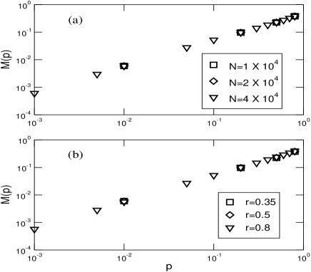
Figure 1: Log-log plots of $M(p)~{}\textrm{vs}~{}p$ for: (a) a network with $k_{min}=1$, $r=0.5$ and different $N$ (b) a network with $k_{min}=1$, $N=10^{4}$ and different $r$

Figure 2: Log-log plot of $M(p)~{}\textrm{vs}~{}p$ for $k_{min}=1$, $N$ varying from $1\times 10^{4}$ up to $4\times 10^{4}$ and $r=0.35,\,0.5$ and $0.8$ . It shows the best fit of the coalesced sets.

We can see from Fig. 1 that $M(p)$ behaves as a power function of type $p^{m}$ for the entire range of $p$. By comparing the behavior of the smallest network ($N=1\times 10^{4}$) with the largest one ( $N=4\times 10^{4}$) we can see that finite size effects are small for $M(p)$. Moreover, it seems that the exponent $m$ does not depend on $r$. In order to evaluate the exponent $m$ we coalesce all different sets ($N$ varying from $10^{4}$ up to $4\times 10^{4}$ and $r$ from 0.35 up to 0.8) and we do a best fit. This is shown in Fig. 2. We obtain that

$$M(p)=ap^{m},$$

with $a=0.46\pm 0.01$ and $m=0.96\pm 0.01$. Note that we have evaluated the exponent by considering approximately 2 orders of magnitude in the $p$ variable and that the fit is very good. In fact, in all fitted data, we obtained a correlation coefficient larger that $0.999$.

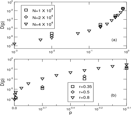
Figure 3: (a) Log-log plot of $D(p)~{}\textrm{vs}~{}p$ for a network with $k_{min}=1$, $r=0.5$ and different $N$; (b) Linear-log plot of $D(p)~{}\textrm{vs}~{}p$ for a network with $k_{min}=1$, $N=2\times 10^{4}$ and different $r$.

Plots of $D(p)$ versus $p$ are shown in Fig. 3 for $r=0.5$ and networks with different sizes. We can see that $D(p)$ has a power law behavior ($D(p)\sim p^{d}$) only when the probability $p$ is close to $p=0$. Outside of these region, $D(p)$ grows exponentially. By comparing the behavior of networks with different sizes, we observe that finite size effects are now important.

Figure 4: (a) Linear-log plot of $D(p)+B~{}\textrm{vs}~{}p$ for a network with $k_{min}=1$, $r=0.5$ and different $N$; (b) Log-log plot of $D(p)+B~{}\textrm{vs}~{}p$ for a network with $k_{min}=1$, $N=2\times 10^{4}$ and different $r$.

It turns out that all results can be well fitted by

$$D(p)=B\exp(Cp)-B,$$

with $C$ and $B$ depending on the size of the network and on the parameter $r$. This can be seen in Fig. 4. When $p\approx 0$, we have that $D\sim BCp$.

III.2 Data and results for $k_{min}=2$

The simulation for the networks with $k_{min}=2$ were realized in the same way that for $k_{min}=1$, and the probability $p$ was taken in the interval $[0.01,0.9]$ for $r=0.2$, $0.5$ and $0.8$. The range of $p$ is rather narrow in this case, since the dynamics for $k_{min}=2$ is more sensible to $p$ values, leading to $M(p,t)\rightarrow 0$ and $D(p,t)\rightarrow 0$ when $p\sim 0.001$. This behavior perhaps is related to the one found for RBN with only part of the canalyzing functions as update functions, $K=2$, and small $p_{+}$, where $p_{+}$ is the probability that a connection be excitatory greil-drossel .

Figure 5: Log-log plot of $M(p)~{}\textrm{vs}~{}p$ for $k_{min}=2$, $N$ varying from $1\times 10^{4}$ up to $4\times 10^{4}$ and $r=0.2,\,0.5$ and $0.8$ . It shows the best fit of the coalesced sets.

Fig. 5 is similar to fig. 2, where all sets of $r$ and $N$ are coalesced in one plot. We can see that the finite size effect is very small and we have

$$M(p)=ap^{m},$$

with $a=0.70\pm 0.02$ and $m=1.79\pm 0.01$.

Figure 6: Linear plot of $D(p)~{}\textrm{vs}~{}p$ for $k_{min}=2$, $r=0.2$, $0.5$ and $0.8$ for $N=10^{3}$.

As we can see in Fig. 6, the Hamming distance $D(p)$ follows a linear dependence with $p$ for large values of $p$ (the plot shows $p\geq 0.3$). In this region the behavior of $D(p)$ is almost independent of $r$, and we have:

$$D(p)\sim ap,$$

where $a=0.78\pm 0.02$, $0.76\pm 0.02$ and $0.72\pm 0.02$ for $r=0.2$, $0.5$ and $0.8$ respectively. However, the behavior of $D(p)$ for $p\leq 0.3$ does not provide any suitable fit since for low values of $p$ we have a high concentration of AND function and a low concentration of XOR function, leading most of nodes to the $0$ state.

Note that results discussed in this section are valid for other values of $r$. We discuss only the cases $r=0.5$ (linear preferential attachment), one case with $r<0.5$ ($r=0.35$ or $r=0.2$) and one case with $r>05$ ($r=0.8$ or $r=0.7$) because they represent typical behaviors. We have simulated other cases, with less samples, and the results are similar. Although we present $D(p,t)$ for the initial condition $D(p,0)=1$, we have also simulated cases with $D(p,0)>1$. We find similar results, probably because this new initial condition is a later state of the initial condition with the smallest Hamming distance. In the next section we will develop a mean-field approach in order to see if its results agree with the numerical ones just obtained.

IV Mean-field approximation

In this section we present a mean-field approach (MF). It is based on a work of Derrida and Pomeau derr , in which an annealed approximation was done for the Kauffman $NK$ model. The NK model is a cellular automaton with $N$ nodes holding logical variables. Each node $\sigma_{i}$ is connected with another $K$ nodes of the network meaning that all nodes have the same connectivity $K$. The dynamics is given by Eq. (1) where $G_{i}$ is a random Boolean function. Although the model is defined by quenched disorder, i.e, the Boolean function $G_{i}$ and the $K$ nodes connected to each node $\sigma_{i}$ are only randomly chosen at the initial time, in the Derrida and Pomeau approximation it is assumed an annealed disorder. It means that the Boolean function and the $K$ nodes are randomly chosen at each time step. Moreover, in such approximation the effect of the Boolean functions on a node is described by probabilities that the output be 0 and 1. The approximation to our problems is similar to that of Derrida and Pomeau. However, a difference appears in the application of the Boolean functions. Instead of using a probabilistic description for the effect of the Boolean functions, we determine the effect of applying the XOR and AND operators in each configuration. We will first discuss the case $k_{min}=2$ because it is more illustrative than the more simple case $k_{min}=1$.

IV.1 Average density of $1$’s for $k_{min}=2$

Let us start our evaluation for the model without a scale-free topology. The dynamics is given by equations (1) and (2). Suppose that the configuration of the system at time $t$, $\{\sigma_{i}(t)\}$, consists of $n$ nodes with $\sigma=1$ and $N-n$ nodes with $\sigma=0$. In order to study the density of $1$’s, we can separate the configuration $\{\sigma_{i}(t)\}$ in two sets: (i) set $\mathcal{A}(t)$ where all the nodes have $\sigma=0$, and (ii) set $\mathcal{B}(t)$ where all the nodes have $\sigma=1$. Now we must randomly choose $K$ nodes that are linked to the node $i$. The probability that a given link comes from set $\mathcal{A}(t)$ is $1-x=(N-n)/N$ and the probability that it comes from $\mathcal{B}(t)$ is $x=n/N$. Since each node has $K$ links, the list $P_{K}$ of the probabilities of the possible link configurations is

$$P_{K}=\left\{{K\choose K}(1-x)^{K},~{}~{}{K\choose K-1}(1-x)^{K-1}x,~{}\right.$$ (5)

$$\left.{K\choose K-2}(1-x)^{K-2}x^{2},~{}~{}...,{K\choose 0}x^{K}\right\}.$$

We must now evaluate the output of each possible configuration under the application of operators AND and XOR. The Boolean function AND generates an output $1$ if all inputs come from set $\mathcal{B}(t)$. The probability of this configuration is given by the last term of the list (5). The function XOR, however, produces $1$ as output when its number of inputs equal to $1$ is an odd number, meaning that the number of links coming from set $\mathcal{B}(t)$ is odd. Therefore the probability $X$ of obtaining $1$ as output is

$$X=p\sum_{\begin{subarray}{c}m=1\\ m~{}odd\end{subarray}}^{K}{K\choose m}(1-x)^{K-m}x^{m}+qx^{K},$$

where $p$ and $q=1-p$ are the probabilities related to the XOR and AND operators. Since we have that

$$(y\pm x)^{K}=\sum_{m=0}^{K}{K\choose m}y^{K-m}(\pm x)^{m},$$

the sums of the even and odd terms are given by

$$\sum_{\begin{subarray}{c}m=0\\ m~{}even\end{subarray}}^{K}{K\choose m}y^{K-m}x^{m} = \frac{(y+x)^{K}+(y-x)^{K}}{2},$$ (6)

$$\sum_{\begin{subarray}{c}m=1\\ m~{}odd\end{subarray}}^{K}{K\choose m}y^{K-m}x^{m} = \frac{(y+x)^{K}-(y-x)^{K}}{2}.$$ (7)

It follows that $X=\frac{p}{2}[1-(1-2x)^{K}]+qx^{K}$. Assuming homogeneity, we can identify $X$ as $M(p,t+1)$, the fraction of $1$’s at time $t+1$. Then we obtain that $M(p,t+1)$ depends only on $M(p,t)$ as

$$M(p,t+1)=\frac{p}{2}\{1-[1-2M(p,t)]^{K}\}+q{M(p,t)}^{K}.$$ (8)

Finally let us consider the scale-free topology. Each node now has $k$ links with probability $P(k)$. Therefore the above equation can be written as

$$M(p,t+1) = \frac{p}{2}\left\{1-\sum_{k=2}^{\infty}P(k)[1-2M(p,t)]^{k}\right\}$$ (9)

$$+ q\sum_{k=2}^{\infty}P(k){M(p,t)}^{k}.$$

IV.2 Average Hamming distance for $k_{min}=2$

The calculation of the Hamming distance is done in a similar way. Let us again first study the model without scale-free topology. At time $t$ we are interested in the configuration $\{\sigma(t)\}$ resulting from the evolution of the initial configuration, and in the configuration $\{\overline{\sigma(t)}\}$, which appears from the evolution of the initial damaged copy. Suppose that they differ by $n$ nodes. Following Derrida and Pomeau derr , we define two sets: $\mathcal{E}(t)$ and $\mathcal{F}(t)$. The first one is the set of all nodes of $\{\sigma(t)\}$ and $\{\overline{\sigma(t)}\}$ that have the same values. The set $\mathcal{F}(t)$ is composed by the $n$ nodes that have different values in the two configurations. Therefore the nodes which have all links coming from set $\mathcal{E}(t)$ will have the same values at time $t+1$ in the $\{\sigma(t)\}$ and $\{\overline{\sigma(t)}\}$ configurations and they will not contribute to the Hamming distance. On the other hand, the Hamming distance could be changed by the nodes which have at least one link coming from the $n$ nodes of $\mathcal{F}(t)$.

Let us also define $E_{0}$ and $E_{1}$ as the number of nodes in the set $\mathcal{E}(t)$ with the values $0$ and $1$, respectively. $F_{0}$ is the number of nodes in the set $\mathcal{F}(t)$ that have $\sigma(t)=0$, and $F_{1}$ is the number of nodes with $\sigma(t)=1$. Observe that $F_{0}+F_{1}=n$ and $E_{0}+E_{1}=N-n$. The next step is to focus in a particular node $i$ and to determine the probability of have $K$ randomly chosen nodes linked to it. The probability that a link comes from set $\mathcal{E}(t)$ with the corresponding node having value $1$ is $z_{1}=E_{1}/N$. If the link comes from the same set but the node of $\mathcal{E}(t)$ has value $0$, the probability will be $z_{0}=E_{0}/N$. $w_{0}=F_{0}/N$ and $w_{1}=F_{1}/N$ are the probabilities that a link comes from $\mathcal{F}(t)$ when the corresponding elements of the set have values $0$ and $1$, respectively. Since $E_{0}+E_{1}+F_{0}+F_{1}=N$, it is obvious that $z_{0}+z_{1}+w_{0}+w_{1}=1$.

We are interested in the evaluation of $W_{1}$, the probability that $\sigma_{i}(t+1)=1$ and $\overline{\sigma+_{i}(t+1)}=0$, and of $W_{0}$, the probability that $\sigma_{i}(t+1)=0$ and $\overline{\sigma_{i}(t+1)}=1$. The first step is to study the situation in which the node $i$ has $K-1$ links in set $\mathcal{E}(t)$ and only one link in $\mathcal{F}(t)$. The list of the probabilities of the possible link configurations is

$$P_{1}^{(1)} = \left\{{K\choose 1}w_{0},~{}{K\choose 1}w_{1}\right\}\left\{z_{0}^{K-1},~{}{K-1\choose 1}z_{0}^{K-2}z_{1},\right.$$ (10)

$$\left.{K-1\choose 2}z_{0}^{K-3}z_{1}^{2},~{}\ldots,~{}z_{1}^{K-1}\right\},$$

where we must multiply each element of the first list by each element of the second one. We must now evaluate the output of each possible configuration under the operator XOR. For the first configuration (${K\choose 1}w_{1}z_{0}^{K-1}$), the XOR operation furnishes that $\sigma_{i}=1$ in configuration $\{\sigma(t+1)\}$ and $\sigma_{i}=0$ in $\{\overline{\sigma(t+1)}\}$, implying that $p{K\choose 1}w_{1}z_{0}^{K-1}$ will contribute to $W_{1}$. Note that the extra probability $p$ is related to the XOR operator. The second configuration (${K\choose 1}w_{1}{K-1\choose 1}z_{0}^{K-2}z_{1}$) will contribute to $W_{0}$ because the application of XOR give-us that $\sigma_{i}=0$ in $\{\sigma(t+1)\}$ and $\sigma_{i}=1$ in $\{\overline{\sigma(t+1)}\}$. Since the third term (${K\choose 1}w_{1}{K-1\choose 2}z_{0}^{K-3}z_{1}^{2}$) will contribute to $W_{1}$, it is easy to infer that for configurations beginning with $w_{1}$, the terms $z_{1}^{m}$ with $m$ even contribute to $W_{1}$ and the ones with $m$ odd enter in $W_{0}$. A similar analysis shows that for configurations beginning with $w_{0}$, the terms with $m$ even contribute to $W_{0}$ and the ones with $m$ odd enter in $W_{1}$. When we apply the AND operator, only the terms $w_{1}z_{1}^{K-1}$ and $w_{0}z_{1}^{K-1}$ give no null contributions to $W_{1}$ and $W_{0}$, respectively. Therefore the contributions of the list (10) to $W_{1}$ and $W_{0}$ can be written as

$$W_{1}^{(1)} = {K\choose 1}\left[pw_{1}\sum_{\begin{subarray}{c}m=0\\ m~{}even\end{subarray}}^{K-1}{K-1\choose m}z_{0}^{K-m}z_{1}^{m}\right.$$

$$\left.+pw_{0}\sum_{\begin{subarray}{c}m=1\\ m~{}odd\end{subarray}}^{K-1}{K-1\choose m}z_{0}^{K-m}z_{1}^{m}+qw_{1}z_{1}^{K-1}\right],$$

$$W_{0}^{(1)} = {K\choose 1}\left[pw_{0}\sum_{\begin{subarray}{c}m=0\\ m~{}even\end{subarray}}^{K-1}{K-1\choose m}z_{0}^{K-m}z_{1}^{m}\right.$$

$$\left.+pw_{1}\sum_{\begin{subarray}{c}m=1\\ m~{}odd\end{subarray}}^{K-1}{K-1\choose m}z_{0}^{K-m}z_{1}^{m}+qw_{0}z_{1}^{K-1}\right].$$

Using Equations (6) and (7), $W_{1}^{(1)}$ can be written as

$$W_{1}^{(1)} = {K\choose 1}\left[\frac{p}{2}(w_{1}+w_{0})(z_{0}+z_{1})^{K-1}\right.$$

$$\left.+\frac{p}{2}(w_{1}-w_{0})(z_{0}-z_{1})^{K-1}+qw_{1}z_{1}^{K-1}\right].$$

The equation for $W_{0}^{(1)}$ is obtained by changing $w_{0}$ by $w_{1}$, and $w_{1}$ by $w_{0}$ in the above equation.

The second step is to study the situation in which the node $i$ has $K-2$ links in set $\mathcal{E}(t)$ and two links in $\mathcal{F}(t)$. Now, the list of the probabilities of the possible link configurations is

$$P_{1}^{(2)}={K\choose 2}\left\{w_{0}^{2},~{}2w_{0}w_{1},~{}w_{1}^{2}\right\}\left\{z_{0}^{K-2},\right.$$ (11)

$$\left.{K-2\choose 1}z_{0}^{K-3}z_{1},~{}{K-2\choose 2}z_{0}^{K-4}z_{1}^{2},~{}\ldots,~{}z_{1}^{K-2}\right\}.$$

There is no contribution of the XOR operator. The AND operator furnishes that only two configurations ($w_{1}^{2}z_{1}^{K-2}$ and $w_{0}^{2}z_{1}^{K-2}$), multiplied by probability $q$, contribute to $W_{1}$ and $W_{0}$. Therefore we find that

$$W_{1}^{(2)}={K\choose 2}qw_{1}^{2}z_{1}^{K-2},~{}~{}{\rm and}~{}~{}W_{0}^{(2)}={K\choose 2}qw_{0}^{2}z_{1}^{K-2}.$$

The third step is to evaluate the probabilities generated by the application of XOR and AND in the situation in which the node $i$ has $K-3$ links in set $\mathcal{E}(t)$ and three links in $\mathcal{F}(t)$. This situation is similar to the first one. We obtain that

$$W_{1}^{(3)} = {K\choose 3}\left[\frac{p}{2}(w_{1}+w_{0})^{3}(z_{0}+z_{1})^{K-3}\right.$$

$$\left.+\frac{p}{2}(w_{1}-w_{0})^{3}(z_{0}-z_{1})^{K-3}+qw_{1}^{3}z_{1}^{K-3}\right].$$

The result for $W_{0}^{(3)}$ is identical with the previous one if we change $w_{0}$ by $w_{1}$, and $w_{1}$ by $w_{0}$.

The fourth step is similar to the second one, and so on. Since $W_{1}=\sum_{m=1}^{K}W_{1}^{(m)}$, we have that

$$W_{1}=\frac{p}{2}\sum_{m,odd}^{K}{K\choose m}\left[(w_{1}+w_{0})^{m}(z_{0}+z_{1})^{K-m}\right.$$

$$\left.+(w_{1}-w_{0})^{m}(z_{0}-z_{1})^{K-m}\right]+q\sum_{m=1}^{K}{K\choose m}w_{1}^{m}z_{1}^{K-m}.$$

To obtain $W_{0}$ we substitute $w_{0}$ by $w_{1}$, and $w_{1}$ by $w_{0}$ in this equation. Using again Eq. (6), we obtain that

$$W_{1} = q[(w_{1}+z_{1})^{K}-z_{1}^{K}]+\frac{p}{4}\{1-[1-2(w_{1}+w_{0})]^{K}$$ (12)

$$+ [1-2(z_{1}+w_{0})]^{K}-[1-2(z_{1}+w_{1})]^{K}\},$$

$$W_{0} = q[(w_{0}+z_{1})^{K}-z_{1}^{K}]+\frac{p}{4}\{1-[1-2(w_{1}+w_{0})]^{K}$$ (13)

$$+ [1-2(z_{1}+w_{1})]^{K}-[1-2(z_{1}+w_{0})]^{K}\}.$$

Assuming homogeneity, we can identify $W_{1}$ as $w_{1,t+1}$, the fraction of $1$’s of set $\mathcal{F}(t)$ at time $t+1$, and $W_{0}$ as $w_{0,t+1}$. Note that the fraction of $1$’s of the system is given by $M(p,t+1)=z_{1,t+1}+w_{1,t+1}$ and that it was already evaluated (see Eq.(8)). Identifying $z_{1,t+1}$ with $Z_{1}$, we obtain that

$$Z_{1}=M(p,t+1)-W_{1}.$$

Observe that the equations for $W_{1}$, $W_{0}$ and $Z_{1}$ describe completely our system, since the equation for $Z_{0}$ is obtained from the normalization condition. However it is usual to work with variables $M(p,t+1)$, the density of $1$’s and with $D(p,t+1)$, the Hamming distance. From the definition of the Hamming distance we have that $D(p,t+1)=w_{1,t+1}+w_{0,t+1}$, implying that

$$D(p,t+1) = q\{M(p,t)^{K}+[D(p,t)-M(p,t)+2z_{1,t}]^{K}$$

$$- 2z_{1,t}^{K}\}+\frac{p}{2}\{1-[1-2D(p,t)]^{K}\}.$$

The equations for $D(p,t+1)$, $M(p,t+1)$ and $z_{1,t+1}$ also describe completely the system. However, if $w_{1}=w_{0}$ we can see from Eqs. (12) and (13) that $W_{1}=W_{0}$. Solving numerically these equations, we obtain that each initial configuration with $w_{1}\not=w_{0}$ evolves to a fixed point with $W_{1}=W_{0}$. Then we can assume that $w_{0}=w_{1}$, without loss of generality, and the dynamics of the system is described by only two equations, namely

$$D(p,t+1) = 2q\{M(p,t)^{K}-[M(p,t)-\frac{D(p,t)}{2}]^{K}\}$$ (14)

$$+ \frac{p}{2}\{1-(1-2D(p,t))^{K}\},$$

$$M(p,t+1) = qM(p,t)^{K}$$

$$+ \frac{p}{2}\{1-[1-2D(p,t)]^{K}\}.$$

Finally let us consider the model with the scale-free topology. Since each node now have $k$ links with probability $P(k)$, the above equations, which are valid for $w_{1}=w_{0}$, can be written as

$$D(p,t+1) = 2q\left\{\sum_{k=2}^{\infty}P(k)\{M(p,t)^{k}\right.$$ (16)

$$- \left.[M(p,t)-\frac{D(p,t)}{2}]^{k}\}\right\}$$

$$+ \frac{p}{2}-\frac{p}{2}\sum_{k=2}^{\infty}P(k)[1-2D(p,t)]^{k},$$

$$M(p,t+1) = \frac{p}{2}\left\{1-\sum_{k=2}^{\infty}P(k)[1-2M(p,t)]^{k}\right\}$$ (17)

$$+ q\sum_{k=2}^{\infty}P(k){M(p,t)}^{k}.$$

IV.3 $M(p,t)$ and $D(p,t)$ for $k_{min}=1$

The main difference between this case and the previous one is the self-regulation mechanism: the node itself always participates in its own dynamics. Itself and the $K$ nodes connected to it are the control elements of the dynamics. Following a similar procedure of the subsection IV.1, we obtain that

$$M(p,t+1) = \frac{p}{2}\left\{1-\sum_{k=1}^{\infty}P(k)[1-2M(p,t)]^{k+1}\right\}$$ (18)

$$+ q\sum_{k=1}^{\infty}P(k){M(p,t)}^{k+1},$$

where $P(k)$ is the probability that a node had $k$ links.

The evaluation of the Hamming distance follows similar steps of subsection IV.2. For scale-free systems we again have the quantities $W_{0}$, $W_{1}$ and $Z_{1}$. It turns out that when $w_{1}=w_{0}$ we have $W_{1}=W_{0}$. When $w_{1}=w_{0}$, the dynamics of the system is given by Eq. (18) and by

$$D(p,t+1) = 2q\left\{\sum_{k=1}^{\infty}P(k)\{M(p,t)^{k+1}\right.$$ (19)

$$- \left.[M(p,t)-\frac{D(p,t)}{2}]^{k+1}\}\right\}$$

$$+ \frac{p}{2}-\frac{p}{2}\sum_{k=1}^{\infty}P(k)[1-2D(p,t)]^{k+1}.$$

If we put $P(k)=\delta_{k,K}$ in Eqs. (18) and (19), we obtain the results for the model without a scale-free topology. They are similar to the ones obtained for the case without self-regulation, but with $K$ replaced by $K+1$ (see Eqs. (14) and (IV.2)). For scale-free systems, the dynamics with self-regulation is similar to the usual dynamics if we change $k$ by $k+1$, except in the distribution of connectivity $P(k)$ (see Eqs. (16 and 17). Therefore the dynamics with self-regulation is different from the usual case. Let us investigate if this fact is also true for the Kauffman NK model.

IV.4 Kauffman model with self-regulation

The Kauffman NK model consists of $N$ nodes holding logical variables $\sigma_{i}$. Each node is connected with any $K$ nodes of the network. Observe that a node $i$ can have a link to itself with small probability ($K/N$). The dynamics, given by Eq. (1), is determined by a random Boolean function $G_{i}$. In the Derrida and Pomeau annealed approximation derr , the Boolean function and the $K$ nodes are randomly chosen at each time step. The configuration $\{\sigma(t)\}$ is split in the sets $\mathcal{F}(t)$, which consists of nodes having different values of $\sigma$ in configurations $\{\sigma(t)\}$ and $\{\overline{\sigma(t)}\}$, and $\mathcal{E}(t)$ when the previous condition does not hold. Then we are able to define the probabilities $w$ and $z$ that a link of a particular node comes from sets $\mathcal{F}(t)$ and $\mathcal{E}(t)$, respectively. Obviously we have that $z+w=1$. We want to evaluate the probability $W$ that node $i$ will have different values in $\{\sigma(t+1)\}$ and $\{\overline{\sigma(t+1)}\}$. If all $K$ links came from $\mathcal{E}(t)$, $\sigma_{i}(t+1)$ will have the same value in both $\{\sigma(t+1)\}$ and $\{\overline{\sigma(t+1)}\}$. However, if at least one link comes from $\mathcal{F}(t)$, $\sigma_{i}(t+1)$ has a positive probability of having different values in $\{\sigma(t+1)\}$ and $\{\overline{\sigma(t+1)}\}$. Due to the random Boolean function assignment any node can be $0$ or $1$ with probability $1/2$, and the probability that $\sigma_{i}(t+1)$ will have different values in $\{\sigma(t+1)\}$ and $\{\overline{\sigma(t+1)}\}$ is $1/2$. Therefore the probability $W$ is given by

$$W=\frac{1}{2}\left[{K\choose 1}z^{K-1}w+{K\choose 2}z^{K-2}w^{2}+\ldots+w^{K}\right].$$

Assuming that the system is homogeneous, we can identify the fraction of nodes with different values in $\{\sigma(t+1)\}$ and $\{\overline{\sigma(t+1)}\}$, $W$, with the Hamming distance $D(p,t+1)$. Using that $w=D(p,t)$ in the previous equations we obtain the traditional equation of Derrida and Pomeau derr , namely

$$D(p,t+1)=\frac{1}{2}\{1-[1-D(p,t)]^{K}\}.$$

Let us consider now a model with self-regulation. Moreover, each node also has $K$ links connected to any of the $N$ nodes of the network. We focus on node $i$. This node has probabilities $z_{i}=z$ and $w_{i}=w$ to belong to sets $\mathcal{E}(t)$ and $\mathcal{F}(t)$, respectively. We want again to compute $W$. If node $i$ is in set $\mathcal{F}(t)$ it has probability $1/2$ to contribute to $W$, independently of the $K$ links. Otherwise, at least one of the $K$ links must be in set $\mathcal{F}(t)$. Taken in account these two situations, we have that

$$W=\frac{w_{i}}{2}+\frac{z_{i}}{2}\left[{K\choose 1}z^{K-1}w+{K\choose 2}z^{K-2}w^{2}+\ldots+w^{K}\right].$$

Identifying $W$ with $D(p,t+1)$ and $w$ with $D(p,t)$, we find that the Hamming distance is given by

$$D(p,t+1)=\frac{1}{2}\{1-[1-D(p,t)]^{K+1}\}.$$ (20)

Observe that again this expression is similar to the previous one if $K$ is replaced by $K+1$.

Both models can be studied in a scale-free topology. It is easy to obtain that

$$D(p,t+1)=\frac{1}{2}\left\{1-\sum_{k}P(k)[1-D(p,t)]^{\theta}\right\},$$ (21)

where $\theta=k+1$ for the case with self-regulation, and $\theta=k$ otherwise. These results are easily generalized to taken in account the Derrida parameter $p_{d}$ (see Derrida and Pomeau derr ). In this case the probability $1/2$ of Eqs. (20) and (21) must be replaced by the corresponding probability $2p_{d}(1-p_{d})$.

V Mean-field and simulation results

V.1 Results for $k_{min}=2$

The fixed points for the model without a scale-free topology are obtained by putting $M(p,t+1)=M(p,t)=M_{*}$ in the map given by Eq. (8). The fixed point $M_{*}=0$ always exists, and the local stability parameter $\lambda$, given by

$$\lambda=\left.\frac{dM(p,t+1)}{dM(p,t)}\right|_{M_{*}}=pK(1-2M_{*})^{K-1}+Kq{M_{*}}^{K-1},$$

tell us that $M_{*}=0$ is stable for $\lambda=pK<1$. It means that $\lim_{t\to\infty}M(p,t)=0$ for any initial value $M(p,0)$. When $pK>1$ the initial conditions are attracted to a non null fixed point. It means that in the $(p,K)$ plane, there is a curve, given by equation $pK=1$, separating the region in which $M_{*}=0$ is stable from the one that $M_{*}=0$ is not stable. These features can be easily illustrated for $K=2$. In this case, the non null fixed point is given by $M_{*}=(1-2p)/(1-3p)$ and the local stability parameter, evaluated for non null $M_{*}$, is $\lambda=2(1-p)$. Then we have that $\lambda<1$ for $p>1/2$. It implies that for $p>1/2$, the non null fixed point is attractive. For $K>2$ the evaluation of the fixed point and of $\lambda$ were performed numerically.

Table 1: Values of density of $1^{\prime}s$ ($M(p)$) and Hamming distance ($D(p)$) for the model without a scale-free topology with $k_{min}=2$, $N=10000$, and the dynamics described by XOR and AND functions without self-regulation. The subscript sim is the simulated result and the ann refers to annealed (MF) solution. The error in the last digit of an evaluated quantity in the simulations is between parentheses.

$K$	$p$	$M_{ann}$	$M_{sim}$	$D_{ann}$	$D_{sim}$
$2$	$0.0$	0.000	0.000(1)	0.000	0.000(2)
	$0.2$	0.000	0.000(1)	0.000	0.000(2)
	$0.5$	0.002	0.054(3)	0.002	0.060(3)
	$0.7$	0.364	0.362(3)	0.399	0.397(2)
	$1.0$	0.500	0.500(2)	0.500	0.500(1)
$5$	$0.0$	0.000	0.000(1)	0.000	0.000(1)
	$0.2$	0.000	0.017(3)	0.000	0.016(2)
	$0.5$	0.241	0.241(2)	0.242	0.241(2)
	$0.8$	0.402	0.402(2)	0.404	0.404(2)
	$1.0$	0.500	0.500(1)	0.500	0.500(2)
$10$	$0.0$	0.000	0.000(1)	0.000	0.000(1)
	$0.2$	0.084	0.084(1)	0.084	0.083(2)
	$0.5$	0.250	0.249(1)	0.250	0.250(2)
	$0.8$	0.400	0.400(1)	0.400	0.400(1)
	$1.0$	0.500	0.500(1)	0.500	0.500(1)

In table (1) we compare the results of the annealed approximation for three values $K$ with the ones obtained by numerical simulations of $N=10^{4}$ nodes, with the average quantities evaluated after $10^{3}$ mcs in $3000$ samples. In the simulation results, the numbers between parentheses are the errors that affect the last digits. Similar results were obtained for other values of $p$. We can conclude that the MF results for the fraction of $1$’s agree very well with those from the numerical simulations.

The fraction of $1$’s in a scale-free network is described by Eq. (9). Again the fixed point $M_{*}=0$ is always present. $\lambda$ can also evaluated and we have that the $M_{*}=0$ is stable if $p<1/\langle k\rangle$. When $M_{*}=0$ is not stable, we obtain numerically that there is a non null fixed point attracting all the initial conditions. These regions are separated in the $(p,\langle k\rangle)$ plane by a curve described by

$$p\langle k\rangle=1.$$ (22)

In Tab. (2) we compare the results of the annealed approximation with the ones obtained from numerical simulations with $10^{4}$ nodes and $r=0.5$ ($\gamma=3$). The $M_{*}$ results obtained by MF solution agree well with the ones from simulations. Similar results are obtained for other values of $r$.

Table 2: Values of density of $1^{\prime}s$ ($M(p)$) and Hamming distance ($D(p)$) for Boolean dynamics described by XOR and AND functions without self-regulation on scale-free networks with $N=10000$, $k_{min}=2$, and $r=0.5$ ($\gamma=3$). The subscripts sim and ann refer to the simulated and MF results, respectively. The errors evaluated in the simulations are between parentheses.

$p$	$M_{ann}$	$M_{sim}$	$D_{ann}$	$D_{sim}$
$0.2$	0.003	0.038(3)	0.038	0.007(3)
$0.3$	0.075	0.085(3)	0.113	0.039(3)
$0.5$	0.227	0.216(3)	0.242	0.178(3)
$0.7$	0.352	0.350(4)	0.353	0.340(4)
$0.8$	0.406	0.409(4)	0.404	0.414(4)

The Eqs. (14) and (16) for the Hamming distance can be numerically solved to furnish the fixed points in the cases of the models without and with scale-free topology. Note that we are using that $w_{1}=w_{0}$ in both cases. In Tabs. (1) and (2) we can compare the results obtained from the annealed approximation with those obtained by the numerical simulations. We see that they agree well. This conclusion holds for other values of the parameter $p$.

V.2 Results for $k_{min}=1$

In this case we have self-regulation. The fixed points for $M_{*}$ and $D_{*}$, obtained from Eqs. (18) and (19) with $P(k)=\delta_{k,K}$, are displayed in Tab. (3). We can see that MF results are different from the ones obtained from numerical simulations for small $K$ ($K=1$ and $K=3$), although they are similar when $K$ is large ($K=10$). In order to check our analytical approximation, we have also performed numerical simulations with an annealed dynamics. At each mcs we have randomly chosen the $K$ nodes connected with each node of the network. As we can see, the numerical results agree very well with the ones obtained from MF.

Table 3: Values of density of $1^{\prime}s$ ($M(p)$) and Hamming distance ($D(p)$) for the model without a scale-free topology with $k_{min}=1$, $N=10000$, and the dynamics described by XOR and AND functions with self-regulation. The subscript sim is the simulated result and the ann refers to annealed (MF) solution.

$K$	$p$	$M_{ann}$	$M_{sim}$	$D_{ann}$	$D_{sim}$
$1$	$0.0$	0.000	0.002(2)	0.000	0.000(3)
	$0.2$	0.000	0.130(3)	0.000	0.058(3)
	$0.5$	0.002	0.277(4)	0.002	0.114(4)
	$0.8$	0.429	0.406(5)	0.454	0.172(5)
	$1.0$	0.500	0.497(4)	0.500	0.382(5)
$3$	$0.0$	0.000	0.000(2)	0.000	0.000(3)
	$0.2$	0.000	0.100(4)	0.000	0.073(4)
	$0.5$	0.230	0.250(3)	0.232	0.233(3)
	$0.8$	0.405	0.400(3)	0.410	0.399(3)
	$1.0$	0.500	0.500(3)	0.500	0.500(3)
$10$	$0.0$	0.000	0.000(2)	0.000	0.000(3)
	$0.2$	0.088	0.010(2)	0.088	0.099(3)
	$0.5$	0.250	0.250(3)	0.250	0.250(2)
	$0.8$	0.400	0.400(3)	0.400	0.400(3)
	$1.0$	0.500	0.500(3)	0.500	0.500(3)

The same conclusions hold for the scale-free topology. By using Eq. (18) in the analysis of stability of the $M_{*}=0$ fixed point, we obtain that the curve separating the two regions is given by

$$p(\langle k\rangle+1)=1.$$ (23)

Even if we take into account that $\langle k\rangle$ of the above equation begins with $k=1$ and the one of Eq. (22) begins with $k=2$, Eqs. (22) and (23) are different. This implies that self-regulation changes the dynamical behavior.

Table 4 shows the results of computational simulation and the annealed approximation. It can be seen that the values of $M$ and $D$ obtained via MF when $k_{min}=1$ are a bit smaller than the ones of the $k_{min}=2$ case. Another important feature is the relative good agreement between the values of $M$ obtained via simulation and that from annealed approximation. This match does not occur for the Hamming distance. As we can see in Tab. 4, the spreading damage calculated via MF is quite bigger than the one obtained in simulations. We can conclude by analyzing the Hamming distance, that the self-regulated nodes introduce a new dynamical behavior, with distinct properties when compared to the behavior of non-self-regulated ones. Is worth to comment that self-regulation is a common feature in biological networks. Maybe it is a process used in order to increase homeostasis, reducing the effect of a damage introduced in the system.

Table 4: Values of density of $1^{\prime}s$ ($M(p)$) and Hamming distance ($D(p)$) for Boolean dynamics described by XOR and AND functions with self-regulation on scale-free networks with $N=10000$, $k_{min}=1$, and $r=0.5$ ($\gamma=3$). The subscripts sim and ann refer to the simulated and MF results, respectively. The errors evaluated in the simulations are between parentheses.

$p$	$M_{ann}$	$M_{sim}$	$D_{ann}$	$D_{sim}$
$0.2$	0.091	0.097(3)	0.090	0.000(3)
$0.3$	0.141	0.140(2)	0.140	0.000(3)
$0.5$	0.246	0.228(3)	0.243	0.001(3)
$0.7$	0.351	0.325(2)	0.345	0.013(4)
$0.8$	0.401	0.380(2)	0.396	0.042(4)

VI Summary

In this work we studied Boolean dynamics in Kauffman models and in scale-free networks. The dynamical models assigned only $XOR$ and $AND$ operators to the nodes with probability $p$ and $1-p$. Regarding the inputs of the above cited Boolean networks, two types of dynamics were used. In the first one, the state of the nodes was regulated by the state of all nodes connected to them. The second type was similar to the first one, with the difference that the state of the node was used as its own input. Thus, in the first case we did not have self-regulation as in the second one. As shown in the results, these two types of dynamics presented quite different behaviors. In both cases a computational simulation and an analytical mean-field approximation were performed in order to compare the density of $1^{\prime}s$, namely $M$, and the Hamming distance $D$. The results for the dynamics with no self-regulation generated good agreement between simulations and the MF approach. However, the case with self-regulation had a clear disagreement with respect to $D$ and $M$, for small values of $p$.

The authors thank J. F. F. Mendes for useful discussions. We thank the referees for useful suggestions. ACS and JKLS thank to Fundação de Amparo a Pesquisa de MG (FAPEMIG), a Brazilian agency, for partial financial support. JKLS thanks to Conselho Nacional de Pesquisa (CNPq) for partial financial support.
^∗Electronic address: alcidescs@gmail.com
^†Electronic address: jaff@fisica.ufmg.br

References

- (1) A. L. Barabasi and R. Albert, Science 286, 509 (1999).
- (2) A. L. Barabasi and Z. N. Oltvai, Nature Rev. Genet. 5, 101 (2004).
- (3) S. N. Dorogovtsev and J. F. F. Mendes, Adv. Phys. 51, 1079 (2002).
- (4) L. Wardil and J. K. L. da Silva, Braz. J. Phys. 38, 350 (2008).
- (5) A. T. Bernardes, D. Stauffer and J. Kertesz, Eur. Phys. J. B 25, 123 (2002).
- (6) D. J. Watts and S. H. Strogatz, Nature 393, 440 (1998).
- (7) S. Redner, Eur. Phys. J. B 4, 131 (1998).
- (8) B. A. Huberman, P. L. T. Pirolli, J. E. Pitkow and R. M. Lukose, Science 280, 95 (1998).
- (9) R. Albert, H. Jeong and A. L. Barabasi, Nature 401, 130 (1999).
- (10) B. A. Huberman and L. A. Adamic, Nature 401, 131 (1999).
- (11) M. Barthelemy and L. A. N. Amaral, Phys. Rev. Lett. 82, 5180 (1999).
- (12) M. E. J. Newman and D. J. Watts, Phys. Lett. A 263, 341 (1999).
- (13) A. Barrat and M. Weigt, Eur. Phys. J. B 13, 547 (2000).
- (14) L. A. N. Amaral, A. Scala, M. Barthelemy and H. E. Stanley, Proc. Natl. Acad. Sci. USA 97, 11149 (2000).
- (15) L. A. Barbosa, A. Castro e Silva and J. K. L. da Silva, Phys. Rev. E 73, 41903 (2006).
- (16) H. Jeong, B. Tombor, R. Albert, Z. N. Oltvai and A. L. Barabasi, Nature 407, 651 (2000).
- (17) S. A. Kauffman, J. Theor. Biol. 22, 437 (1969).
- (18) A. Castro e Silva, J. K. L. da Silva and J. F. F. Mendes, Phys. Rev. E 70, 66140 (2004).
- (19) K. Iguchi, S. I. Kinoshita and H. S. Yamada, J. Theor. Biol. 247, 138 (2007).
- (20) E. Novikov and E. Barillot, BMC Sis. Biol. 2, 8 (2008).
- (21) B. Drossel and F. Greil, Phys. Rev. E 80, 026102 (2009).
- (22) M. Aldana, Physica D 185, 45 (2003).
- (23) D. S. Lee and H. Rieger, J. Phys. A: Math. Theor. 41, 415001 (2008).
- (24) H. J. Zhou and R. Lipowsky, Proc. Natl. Acad. Sci. USA 102, 10052 (2005).
- (25) S. Kauffman At Home in the Universe, Oxford University Press, New York, 1995.
- (26) I. Shmulevich, E. R. Dougherty and W. Zhang, Proc. IEEE 90, 1778 (2002).
- (27) N. Guelzim, S. Bottani, P. Bourgine and F. Kepes, Nature Genet. 31, 60 (2002).
- (28) P. L. Krapivsky and S. Redner, Phys. Rev. E 63, 066123 (2001).
- (29) F. Greil and B. Drossel, Eur. Phys. J. B 57, 109 (2007).
- (30) B. Derrida and Y. Pomeau, Europhys. Lett. 1, 45 (1986).