The Origin of Magnetic Fields in Galaxies

Abstract

Microgauss magnetic fields are observed in all galaxies at low and high redshifts. The origin of these intense magnetic fields is a challenging question in astrophysics. We show here that the natural plasma fluctuations in the primordial universe (assumed to be random), predicted by the Fluctuation-Dissipation-Theorem, predicts $\sim 0.034~{}\mu G$ fields over $\sim 0.3$ kpc regions in galaxies. If the dipole magnetic fields predicted by the Fluctuation-Dissipation-Theorem are not completely random, microgauss fields over regions $\gtrsim 0.34$ kpc are easily obtained. The model is thus a strong candidate for resolving the problem of the origin of magnetic fields in $\lesssim 10^{9}$ years in high redshift galaxies.

I Introduction

The origin of large-scale cosmic magnetic fields in galaxies and protogalaxies remains a challenging problem in astrophysics (Zweibel & Heiles, 1997; Kulsrud & Zweibel, 2008; de Souza & Opher, 2008; Widrow, 2002). There have been many attempts to explain the origin of cosmic magnetic fields. One of the first popular astrophysical theories to create seed fields was the Biermann mechanism (Biermann, 1950). It has been suggested that this mechanism acts in diverse astrophysical systems, such as large scale structure formation (Peebles, 1967; Rees & Rheinhardt, 1972; Wasserman, 1978), cosmological ionizing fronts (Gnedin, Ferrara & Zweibel, 2000), star formation and supernova explosions (Miranda, Opher & Opher, 1998; Hanayama et al., 2005). Ryu et al. (2008) made simulations showing that cosmological shocks can create average magnetic fields of a few $\mu G$ inside cluster/groups, $\sim 0.1~{}\mu G$ around clusters/groups, and $\sim 10~{}nG$ in filaments. Medvedev et al. (2006) showed that magnetic fields can be produced by collisionless shocks in galaxy clusters and in the intercluster medium (ICM) during large scale structure formation. Arshakian et al. (2009) studied the evolution of magnetic fields in galaxies coupled with hierarchical structure formation. Ichiki et al. (2006) investigated second-order couplings between photons and electrons as a possible origin of magnetic fields on cosmological scales before the epoch of recombination. The creation of early magnetic fields generated by cosmological perturbations have also been investigated (Takahashi et al., 2005, 2006; Clarke, Kronberg, & Böhringer, 2001; Maeda et al., 2009).

In our galaxy, the magnetic field is coherent over kpc scales with alternating directions in the arm and inter-arm regions (e.g.,Kronberg (1994); Han (2008)). Such alternations are expected for magnetic fields of primordial origin (Grasso & Rubinstein, 2001).

Various observations put upper limits on the intensity of a homogeneous primordial magnetic field. Observations of the small-scale cosmic microwave background (CMB) anisotropy yield an upper comoving limit of $4.7~{}nG$ for a homogeneous primordial field (Yamazaki et al., 2006). Reionization of the Universe puts upper limits of $0.7-3~{}nG$ for a homogeneous primordial field, depending on the assumptions of the stellar population that is responsible for reionizing the Universe (Schleicher et al., 2008). Another upper limit for a homogenous primordial magnetic field is the magnetic Jeans mass $\sim 10^{10}M_{\odot}~{}(B/3nG)^{3}$ (Subramanian & Barrow, 1998; Sethi & Subramanian, 2005). Thus, if we are investigating the collapse of a $\sim 10^{7}M_{\odot}$ protogalaxy, the homogeneous primordial magnetic field must be $<0.3~{}nG$ in order for collapse to occur.

Galactic magnetic fields have been suggested to have evolved in three main stages. In the first stage, seed fields were embedded in the protogalaxy. They may have had a primordial origin, as suggested in this paper. Another possibility is that the seed fields could have been injected into the protogalaxies by AGN jets, radio lobes, supernovas, or a combination of the above. Still another possibility is that the seed fields may have been created by the Biermann battery during the formation of the protogalaxy. In the second stage, the seed fields were amplified by compression, shearing flows, turbulent flows, magneto-rotational instabilities, dynamos or by a combination of the above. In the last stage magnetic fields were ordered by a large scale dynamo (Beck, 2006).

Ryu et al. (2008) investigated the amplification of magnetic fields due to turbulent vorticity created at cosmological shocks during the formation of large scale structures. A given vorticity $\omega$ can be characterized by a characteristic velocity $V_{c}$ over a characteristic distance $L_{c}$. Ryu et al. found that $\omega$ typically is

$$\omega\sim 1-3\times 10^{-16}s^{-1},$$ (1)

which corresponds to 10-30 turnovers in the age of the universe. They investigated $L_{c}>$ 1 Mpc $h^{-1}$. We investigate $L_{c}\simeq$ 200 kpc $h^{-1}$ in protogalaxies for a similar vorticity.

We show that a seed field $0.003~{}nG$ over a comoving $2~{}kpc$ region at z $\sim 10$, predicted by the Fluctuation-Dissipation Theorem (de Souza & Opher, 2008), amplified by the small scale dynamo is a good candidate for the origin of magnetic fields in galaxies. K. Subramanian (1997); Subramanian (1999) and Brandenburg & Subramanian (2000) derived the non-linear evolution equations for the magnetic correlations. We use their formulation for the small scale dynamo and solve the nonlinear equations numerically. In §II, we review the creation of magnetic fields due to electromagnetic fluctuations in hot dense equilibrium primordial plasmas, as described in our previous work (de Souza & Opher, 2008). In §III, we discuss the small scale dynamo and in §IV, the important parameters of the plasma to be used in the calculations. In §V, we present our results and in §VI our conclusions.

II Creation of Magnetic Fields Due to Electromagnetic Fluctuations in Hot Dense Primordial Plasmas in Equilibrium

Thermal electromagnetic fluctuations are present in all plasmas, including those in thermal equilibrium. The level of the fluctuations is related to the dissipative characteristics of the plasma, as described by the Fluctuation-Dissipation Theorem (FDT) (Kubo, 1957) [see also Akhiezer et al. (1975); Sitenko (1967); Rostoker et al. (1965); Dawson (1968)].

de Souza & Opher (2008) studied the evolution of these bubbles as the Universe expanded and found that the magnetic fields in the bubbles, created originally at the quark-hadron phase transition (QHPT), had a value $\sim 9~{}\mu$G and a size 0.1 pc at the redshift $\emph{z}\sim 10$ (see Table 1 of (de Souza & Opher, 2008)). Assuming that the fields are randomly oriented, the average magnetic field over a region D is $B=9\mu G~{}(0.1pc/D)^{3/2}$. The theory thus predicts an average magnetic field $0.003~{}nG$ over a $2~{}kpc$ region at $\emph{z}\sim 10$. We assume this seed field and examine its amplification in a protogalaxy by the small scale dynamo, discussed in the next section.

III Small Scale Dynamo

In a partially ionized medium, the magnetic field evolution is governed by the induction equation

$$(\partial{\bf B}/\partial t)={\bf\nabla}\times({\bf v}_{i}\times{\bf B}-\eta{\bf\nabla}\times{\bf B}),$$ (2)

where ${\bf B}$ is the magnetic field, ${\bf v}_{i}$ the velocity of the ionic component of the fluid and $\eta$ is the ohmic resistivity.

Let $L_{c}$ be the coherence scale of the turbulence. Consider a system whose size is $>L_{c}$ where the mean field, averaged over any scale, is negligible. We take $\mathbf{B}$ to be a homogeneous, isotropic, Gaussian random field with a negligible mean average value. For equal time, the two point correlation of the magnetic field is

$$\left\langle B^{\,i}\left(\mathbf{x},t\right)B^{\,j}\left(\mathbf{y},t\right)\right\rangle=M^{\,ij}\left(r,t\right),$$ (3)

where

$$M^{\,ij}=M_{N}\left[\delta^{\,ij}-\left(\frac{r^{\,i}r^{\,j}}{r^{\,2}}\right)\right]+M_{L}\left(\frac{r^{\,i}r^{\,j}}{r^{\,2}}\right)+H\epsilon_{\,ijk}\,r^{\,k},$$ (4)

(K. Subramanian, 1997; Subramanian, 1999; Brandenburg & Subramanian, 2000). $M_{L}\left(r,t\right)$ and $M_{N}\left(r,t\right)$ are the longitudinal and transverse correlation functions, respectively, of the magnetic field and $H\left(r,t\right)$ is the helical term of the correlations. Since $\mathbf{\nabla\cdot{B}}=0,$ we have $M_{N}=\left(1/2\,r\right)\partial\left(r^{\,2}M_{L}\right)/\left(\partial r\right)$ (Monin & Yaglom, 1975). The induction equation can be converted into evolution equations for $M_{L}$ and $H:$

$$\frac{\partial M_{L}}{\partial\,t}\left(r,t\right) = \frac{2}{r^{\,4}}\frac{\partial}{\partial\,r}\left(r^{4}\kappa_{N}\left(r,t\right)\frac{\partial M_{L}\left(r,t\right)}{\partial\,r}\right)$$ (5)

$$+ G(r)M_{L}\left(r,t\right)+4\,\alpha_{N}H\left(r,t\right),$$

and

$$\frac{\partial H}{\partial{\,t}}\left(r,t\right) = \frac{1}{r^{\,4}}\frac{\partial}{\partial{\,r}}\left[r^{\,4}\frac{\partial}{\partial{\,r}}\left[\,2\,\kappa_{N}\left(r,t\right)H\left(r,t\right)\right.\right.$$ (6)

$$- \left.\left.\alpha_{N}\left(r,t\right)M_{L}\left(r,t\right)\right]\,\right],$$

where

$$\kappa_{N}\left(r,t\right)=\eta+T_{LL}\left(0\right)-T_{LL}\left(r\right)+2\,a\,M_{L}\left(0,t\right),$$ (7)

$$\alpha_{N}\left(r,t\right)=2\,C\left(0\right)-2\,C\left(r\right)-4\,a\,H\left(0,t\right),$$ (8)

and

$$G\left(r\right)=-4\left\{\frac{d}{d\,r}\left[\frac{T_{NN}\left(r\right)}{r}\right]+\frac{1}{r^{\,2}}\frac{d}{d\,r}\left[\,r\,T_{LL}\left(r\right)\right]\right\}$$ (9)

(K. Subramanian, 1997; Subramanian, 1999). $T_{LL}(r)$ and $T_{NN}(r)$ are the longitudinal and transverse correlation functions for the velocity field. The functions $T_{NN}$ and $T_{LL}$ are then related in the way described by Subramanian (1999), which we assume here. These equations for $M_{L}$ and $H,$ describing the evolution of magnetic correlations at small and large scales. The effective diffusion coefficient $\kappa_{N}$ includes microscopic diffusion $(\eta),$ a scale-dependent turbulent diffusion $\left[T_{LL}\left(0\right)-T_{LL}\left(r\right)\right],$ and a ambipolar drift $2aM_{L}\left(0,t\right),$ which is proportional to the energy density of the fluctuating fields. Similarly, $\alpha_{N}$ is a scale-dependent $\alpha$ effect, proportional to $[\,2\,C\left(0\right)-2\,C\left(r\right)].$ The nonlinear decrement of the $\alpha$ effect due to ambipolar drift is $4aH\left(0,t\right),$ proportional to the mean helicity of the magnetic fluctuations. The $G\left(r\right)$ term in equation (5) allows for rapid generation of small scale magnetic fluctuations due to velocity shear (Zel’dovich et al., 1983; Kazantsev, 1968; Brandenburg & Subramanian, 2000; Subramanian, 1999).

This turbulent spectrum simulates Kolmogorov turbulence (Vainstein, 1982). As in the galactic interstellar medium, the protogalactic plasma is expected to have Kolmogorov-turbulence, driven by the shock waves originating from the instabilities, associated with gravitational collapse.

In the galactic context, we can neglect the coupling term $\alpha_{N}H$ as a very good approximation since it is very small and consider only the evolution of $M_{L}$ (Subramanian, 1999).

For turbulent motions on a scale $L$ and a velocity scale $v$, the magnetic Reynolds number (MRN) is $R_{m}=vL/\eta$. There is a critical MRN, $R_{c}\approx 60$, so that for $R_{m}>R_{c}$ (Subramanian, 1999), modes of the small scale dynamo can be excited. The fluctuating field, correlated on a scale $L$, grows exponentially with a growth rate $\Gamma_{L}\sim v/L$ (Subramanian, 1999).

IV The Parameters of the Turbulent Plasma

We use the fiducial parameters, suggested in the literature for the plasma that was present in the protogalaxy (Malyshkin & Kulsrud, 2002; Schekochihin et al., 2002): total mass M $\sim 10^{12}~{}M_{\odot}$, temperature T $\sim 10^{6}$ K, and size $L_{c}\sim 200~{}kpc$. The ion kinematic viscosity is $\sim 5\times 10^{26}~{}cm^{2}/s$, the Spitzer resistivity $\eta_{s}=6.53\times 10^{12}~{}T^{-3/2}\ln\Lambda~{}cm^{2}s^{-1}$ $\sim 8\times 10^{4}~{}cm^{2}s^{-1}$, and the typical eddy velocity $V_{c}\sim 10^{7}~{}cm/s$.

V Results

In Fig. 1, we evaluate $M_{L}$ for various values of r and in Fig. 2 for various values of $V_{c}$, solving numerically equation (5). In Fig 3 we evaluate the mean value of the magnetic field as a function of r and t. Our previous work (de Souza & Opher, 2008) showed that the natural fluctuations of the primordial plasma predicted by the Fluctuation-Dissipation Theorem produces a cosmic web of randomly oriented dipole magnetic fields. The average field over a region $\sim 2$ kpc is predicted to be $0.003~{}nG$. We assume this seed field and examine its amplification by the small scale dynamo in s protogalaxy. This seed field corresponds to an $M_{L}(\sim B^{2})\simeq 10^{-23}~{}G^{2}$. Of particular interest is thus the growth of $M_{L}$ with an initial value $M_{L0}\sim 10^{-23}~{}G^{2}$ in Figs. 1 and 2, for initial magnetic fields $B_{0}\sim 3\times 10^{-12}(2kpc/r)^{3/2}~{}G$ of size $r$ in Fig. 3.

VI Conclusions and Discussion

It was shown previously that the magnetic fields, created immediately after the quark-hadron transition, produce relatively intense magnetic dipole fields on small scales at $\emph{z}\sim 10$ (de Souza & Opher, 2008). We show here that the predicted seed fields of size $\sim 2$ kpc and intensity $0.003~{}nG$ at z $\sim 10$ can be amplified by a small scale dynamo in protogalaxies to intensities close to observed values. In the small scale dynamo studied, we use the turbulent spectrum given by Subramanian (1999). The characteristic velocity $V_{c}$ and length $L_{c}$, used in the expression for the vorticity $V_{c}/L_{c}$, are $V_{c}\simeq 10^{7}cm/s$ and $L_{c}\simeq$ 200 kpc. This vorticity is comparable to that found by Ryu et al. (2008), studying the formation of large scale structures. The length $L_{c}\simeq 200$ kpc used is a characteristic size of a protogalactic cloud. The turbulent spectrum used simulates Kolmogorov turbulence (Vainstein, 1982). From our Figs. 1 and 2, we find that $M_{L}(\sim B^{2})$ increases from $\sim 10^{-23}~{}G^{2}$ (corresponding to a magnetic field $B\sim 3\times 10^{-12}~{}G$ over a region $L\sim$ 2 kpc) to $M_{L}\sim 10^{18}~{}G^{2}$ (corresponding to a field $\sim 10^{-9}~{}G$ over a region $L\sim 2$ kpc) in $10^{9}$ years. This corresponds to a $\sim 6$ e-fold amplification of $B$ in a relatively short time. Collapsing to form galaxies at redshift $\emph{z}\sim 10$, the density increases by a factor of $\sim 200$ and the magnetic fields are amplified by a factor of $\sim 34$. This predicts $0.03~{}\mu G$ fields over 0.34 kpc regions in galaxies. If the dipole magnetic fields predicted by the Fluctuation-Dissipation Theorem are not completely random, microgauss fields over regions $>0.34$ kpc are easily obtained. The model studied is thus a strong candidate to explain the $\mu G$ fields observed in high redshift galaxies.

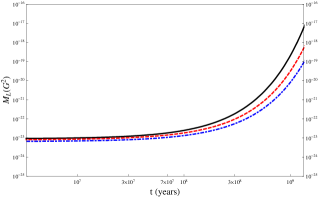
Figure 1: Values of $M_{L}(G^{2}$) as a function of t (years) and r. Solid black line has the reference values: $M_{L}(r,0)=10^{-11}(0.1pc/r)^{3}~{}G^{2}$, $L_{c}=200~{}kpc$, r = 3 kpc, and $V_{c}=10^{7}~{}cm/s$ in Eqs. (36)-(38). Dashed red line is for $r=4~{}kpc$, and the dotted blue line for $r=~{}5kpc$.

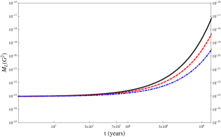
Figure 2: Values of $M_{L}(G^{2}$) as a function of t (years), varying $V_{c}$. Solid black line has the reference values in Fig. 1. Dashed red line is for $V_{c}=8\times 10^{6}~{}cm/s$. Dotted blue line is for $V_{c}=6\times 10^{6}~{}cm/s$.

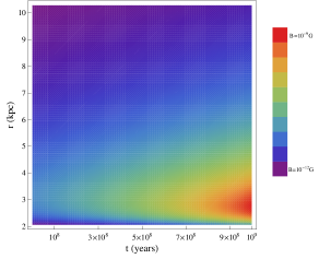
Figure 3: Values of B(G) as a function of t (years) and r(kpc) for reference values of Fig. 1.