Steady–state simulations using weighted ensemble path sampling

Divesh Bhatt, Bin W. Zhang, and Daniel M. Zuckerman

Department of Computational Biology, University of Pittsburgh

Abstract

We extend the weighted ensemble (WE) path sampling method to perform rigorous statistical sampling for systems at steady state. The straightforward steady–state implementation of WE is directly practical for simple landscapes, but not when significant metastable intermediates states are present. We therefore develop an enhanced WE scheme, building on existing ideas, which accelerates attainment of steady state in complex systems. We apply both WE approaches to several model systems confirming their correctness and efficiency by comparison with brute–force results. The enhanced version is significantly faster than the brute force and straightforward WE for systems with WE bins that accurately reflect the reaction coordinate(s). The new WE methods can also be applied to equilibrium sampling, since equilibrium is a steady state.

1 Introduction

Steady–state phenomena are ubiquitous in biological and chemical systems. In biological systems, this is rather unsurprising due to the approximate homeostasis observed at multiple scales (population level, cellular level, and molecular level). At a molecular level, homeostasis results in a protein being constantly removed (for “consumption” downstream) after formation, and new protein is formed at a constant rate. Enzymatic reactions^{1, 2} inside the cell occur at a steady state if the concentration of reactants remains constant and the product is continually removed (as is the case under normal homeostatic conditions). The movement of motor proteins^{1, 3} under saturating ATP conditions typical of the cell is also well described by steady state. Additionally, some in vitro experiments are run at steady state – for example, studies of enzymatic reactions described by Michaelis–Menten kinetics.^{3, 2}

From a theoretical perspective, the steady stare is not simply a “special case” but is fundamentally connected to other ensembles. First and most obviously, equilibrium is itself a steady state. But more interestingly, the trajectories exhibited in a steady state are identical to those which would occur in a single–molecule or first–passage scenario. This was formalized by Hill,⁴ who showed that the flux of probability from state A to B in a steady state is exactly equal to the inverse mean–first–passage time (MFPT) from A to B if the trajectories arriving at B are immediately fed back into A. (As we recently showed, equilibrium can also be exactly decomposed into two steady states⁵). In this manuscript, we present a path sampling procedure that establishes steady state efficiently and allows for the calculation of both steady state and first passage rates.

Computationally, various paths sampling procedures, such as Transition Path Sampling,^{6, 7, 8, 9} Transition Interface Sampling,^{10, 11, 12} Forward Flux Sampling,^{13, 14, 15, 16, 17} and Milestoning^{18, 19} have been developed to compute rate constants for systems with slow kinetics. However, to our knowledge these methods have not been applied to steady state. Recently, Dinner and coworkers^{20, 21} showed that the basic definition of steady state (net zero flux in any region of configurational space) can be used to establish steady state computationally. This procedure is an analog of umbrella sampling for systems not at equilibrium: trajectories in small divisions of configurational space are simulated independently and net zero flux is enforced by monitoring the crossings of trajectories to and from the neighboring regions. Later, vanden–Eijnden and Venturoli²² extended this procedure to allow the calculation of both the steady–state rate and the steady–state flux.

In this work, we extend the previously developed weighted ensemble (WE) path sampling procedure^{23, 24, 25} to perform rigorous statistical sampling of systems at steady state. WE is a particularly attractive path sampling procedure due to its simplicity. In contrast to Dinner and coworkers,^{20, 21} we do not enforce a strict net zero flux in a region. Rather, statistical net zero flux emerges naturally at steady state from WE combined with a simple feedback loop. In essence, net zero flux serves to determine whether the system has reached a steady state.

More importantly, we also develop a probability adjustment procedure to enhance the attainment of steady state using WE simulation. Such a procedure becomes particularly important in systems that show significant intermediates between the two end states, as expected for large biomolecules. Without such a probability adjustment, the steady state is achieved only slowly due to the waiting times required for the regions with the intermediates to reach a stationary value of the probability.

This manuscript is organized as follows. First we show how steady state can be obtained in rigorous statistical simulations using a feedback loop and introduce our method as applied to WE path sampling. Then, we describe in detail the enhanced probability adjustment procedure that leads to a more efficient establishment of steady state. We also describe the different model systems we use: one– and two–dimensional toy systems, and all–atom alanine dipeptide. Following that, we present results for these systems where we also compare the results with brute–force simulations where possible. This is followed by a discussion of the computational issues and possible applications and improvements. Finally, we present our conclusions.

2 Method

2.1 General points

For a system in steady state, the probability of visiting a part of the configuration space remains constant:

$$\frac{dP_{i}}{dt}=\sum_{j}f_{ji}-\sum_{j}f_{ij}=0$$ (1)

where $P_{i}$ is the probability of an arbitrary region $i$, and $f_{ji}$ is the flux of probability from region $j$ to region $i$. Together, the regions $i$ and the set $\{j\}$ completely cover the space but do not overlap. Eq 1 says that the net flux into a region equals the net flux out of the region. As such, equilibrium is a special steady state, where $f_{ij}=f_{ji}=0$ for all pairs of regions. A more general steady state can be obtained even with flows – i.e., with $f_{ij}\neq 0$.

A common steady state is obtained by a feedback loop from the final state to the starting state – if a system reaches the final state, it is fed back into the initial state. This type of steady state is prevalent in biological systems: the proteins formed in the nucleus are removed (for use in cellular processes), subsequently break down, and the amino acid residues are fed back for protein synthesis by the DNA. A more direct feedback loop is observed in case of enzyme catalysis – the enzyme is “fed back” to catalyze more reactants to products (assuming a constant reactant concentration – either under homeostatic conditions in organisms, or via an external reservoir in chemical systems).

These two simple ideas – that steady state is established via a feedback loop, and is obtained when net probability fluxes are zero – are used to develop methods to attain steady states, building on earlier work.²⁰

2.2 Steady state with brute force

Before proceeding to a detailed discussion of simulating a steady state via WE, we note that a steady state can be established using brute–force simulations via a simple feedback loop from the end state to the initial state. If a large number of (independent) brute–force trajectories are started from the initial state, then such a feedback loop eventually establishes a steady state – the distribution of trajectories at any part of the configurational space is independent of time.

For systems with large barriers between the two states, brute–force simulations are not very efficient to study transitions from one state to the other.

2.3 Brief review of generic Weighted Ensemble

Weighted ensemble path sampling is described in greater detail in the original paper by Huber and Kim,²³ and a more recent theoretical review.²⁶ Here we give a brief overview of “ordinary” WE path sampling before discussing our WE methods for steady state. Typically, “start” and “end” states are defined in advance. Further, the whole configuration space is divided into bins, and several trajectories typically are started from one bin with each assigned an equal probability. These trajectories are allowed to evolve for a certain time increment, $\tau$, using the natural system dynamics. After each $\tau$, the trajectories are checked to determine the occupied bins. Each time a bin is occupied, the trajectories entering the bin are split or combined to give a predetermined number of trajectories for that bin. Trajectory probabilities are accordingly allotted in a rigorous statistical manner. That is, no bias is introduced in the evolution of the system, and each part of the configuration space retains the correct probability (as required by the natural, unbiased system dynamics) at all times. As in a Fokker–Planck picture, the system evolution depends solely on the initial condition.²⁶

2.4 ‘Regular’ weighted ensemble attainment of steady state

Weighted ensemble path sampling is naturally adapted to simulating a steady state: any trajectory that enters the end state is fed back into the starting state. Naturally, this requires definitions of the starting and the target states. The starting state can be a finite region of the configuration space or a single configuration (for example, a fully extended protein conformation). The target state must be a finite region of the configuration space to enable a finite flux into the target state. In some cases, the target state may be known in advance – and we consider such systems in this work.

Since the dynamics are not perturbed at all in WE simulations, each point in the configuration space occurs with the correct probability for the condition simulated (whether at equilibrium, in steady state, or for an evolving distribution).²⁶ Correspondingly, because a feedback loop is part of the steady–state definition, it does not perturb the steady state system.

2.5 ‘Enhanced’ weighted ensemble attainment of steady state

In the presence of one or more significant (metastable) intermediates, a steady state can only be achieved after the intermediate state is substantially populated. In such cases, regular WE simulation is still quite inefficient due to the “relaxation” time required from the initial conditions (whereas the steady state solution is completely determined by the feedback condition). This relaxation time can be eliminated if the initial conditions are chosen to approximate the steady state probability distribution.

As a simple example, consider a system with 4 discrete states. State 1 is the starting state and state 4 is the target state. In case of Markovian dynamics, the rate of change of probability in any state is exactly described by the reformulation of eq 1:

$$\frac{dP_{i}}{dt}=\sum_{j}k_{ji}P_{j}-\sum_{j}k_{ij}P_{i}.$$ (2)

where $k_{ij}$ is the rate of transition from state $i$ to state $j$. For simplicity of the following discussion, we assume that all $k_{ij}$ are equal. At steady state, $P_{4}\equiv 0$, and the solution of eq 2 gives $\{P_{1},P_{2},P_{3},P_{4}\}=\{1/2,1/3,1/6,0\}$. A procedure that utilizes an initial condition close to $\{1/2,1/3,1/6,0\}$ effectively eliminates any relaxation time to steady state, whereas the initial conditions of $\{1,0,0,0\}$ may require a substantial relaxation time, depending on the magnitude of the rates.

Motivated by the above discussion and previous work,²⁰ we utilize eq 2 to estimate the steady state probabilities in regions (or bins) of the configurational space. The transition matrix elements, $k_{ij}$, are determined by running unbiased dynamics on trajectories in a bin $i$ for a time increment $\tau$ and estimating the conditional probability to transition to bin $j$. Because generic WE always uses unbiased dynamics, these transition matrix elements can, for example, be computed by setting up a short WE run from arbitrary initial conditions – we elaborate upon this shortly. From the obtained values of $k_{ij}$, estimates for $P_{i}$ are obtained via the use of eq 2. Specifically, if B denotes the target, and A denotes the initial bin, then eq 2 is used for all bins except A and B. For the target bin, $P_{\mathrm{B}}=0$, and the sum of all bin probabilities is 1 (i.e., $P_{\mathrm{A}}+\sum_{i\neq\mathrm{A}}P_{i}=1$). With $N$ bins, this system of $N-1$ linear algebraic equations with $N-1$ unknowns ($P_{\mathrm{B}}=0$) can be solved by standard methods such as Gauss Elimination.

The obtained values of probabilities in each bin thus obtained constitute a near steady–state initial condition. The system is then allowed to relax using regular weighted ensemble until steady values are obtained. To the extent that the estimates of bin probabilities are accurate, the relaxation time is minimized.

There are two important technical issues that determine the appropriateness of the calculated transition matrix of rates for use in eq 2 to determine $P_{i}$ values. One is related to the Markovian approximation inherent in eq 2: ideally, the rate $k_{ij}$ for transitions from bin $i$ to bin $j$ should be calculated only after the intra–bin relaxation time, $\tau_{i}$ (i.e., $\tau>\tau_{i}$). This issue of the applicability of the rate equation was also discussed by Buchete and Hummer.²⁷ Furthermore, several transitions from bin $i$ must be observed to obtain good statistics. Clearly, a longer wait time between recording transitions, as well as a studying larger number of transitions will give a more accurate estimate of the transition matrix elements at the cost of increasingly longer time to calculate the steady state distribution. However, we find that a reasonable estimate of the steady state distribution via the transition matrix in a short amount of time (compared to establishment of steady state via regular WE) can still be obtained. Some of the complications just discussed are artifacts of our (simple) implementation: we use a single WE $\tau$ interval for $k_{ij}$ estimate, but better “book keeping” will readily permit the use of multiple $\tau$.

The arbitrary initial conditions for computing rate matrix elements can be delta function at the starting state, or obtained via running dynamics at elevated temperatures to “fill” up the space initially. Further, after the initial conditions for rate matrix computation are obtained, short brute–force dynamics from these initial conditions may repeatedly be performed to obtain statistically meaningful rates. The only requirement for an appropriate estimate of the rate matrix elements is that dynamics be unbiased at the temperature of interest while computing the rates.

2.6 Equilibrium sampling

The procedure outlined for enhanced WE attainment can also be utilized for performing equilibrium sampling. Instead of setting the probability of the target bin to zero, we use the expression for $dP_{\mathrm{B}}/dt=0$ from eq 2 (as for every other bin). This system of $N$ linear algebraic equations with $N$ unknowns can, again, be solved using standard methods. An accurate estimate of bin populations gives the exact equilibrium distribution. In most problems, this requires a “relaxation” to equilibrium. However, a good estimate can dramatically reduce the relaxation time. We mention that the use of rates to estimate the equilibrium probability distribution was also explored by Buchete and Hummer²⁷ and by Pande and coworkers.²⁸

2.7 Analysis of WE efficiency versus brute force to obtain steady state

There is an intimate connection between steady–state and first–passage kinetics, which permits a fairly direct comparison between our WE simulations and traditional brute–force simulations. In particular, as described in the Introduction, Hill⁴ showed that the probability arriving per unit time (i.e., the flux) into the ‘end’ state in a steady state with immediate feedback in exactly equal to the ‘traditional’ rate or inverse mean-first-passage time. In the notation of eq 1, this can be written as

$$\sum_{i\neq\mathrm{B}}f_{i\mathrm{B}}(\mathrm{SS})=k_{\mathrm{AB}}=\frac{1}{\mathrm{MFPT\;A}\rightarrow\mathrm{B}},$$ (3)

where SS denotes that the fluxes $f_{i\mathrm{B}}$ occur in steady state. Our WE simulations yield all the steady state fluxes $f_{ij}$(SS), which enable quite precise estimates of the brute–force rate $k_{\mathrm{AB}}$.

There are several different measures for comparing the efficiency of enhanced WE path sampling to brute–force simulations. One measure is the comparative transient time that these methods require to first reach within a certain precision of the steady–state flux. Another measure is the comparative time that enhanced WE and brute–force simulations require to attain a certain level of precision after the transients have decayed. A final comparison is via the time either method takes to “find” a pathway between the initial and the final state.

We mainly focus on the first of these measures to compare the efficiency of enhanced WE to brute–force simulations: the comparative time required by these two methods to first reach within a certain precision of the steady–state flux. The reason for this choice is that although we will explicitly obtain both timescales (first approach to steady–state flux, as well as sampling after transients) for enhanced WE simulations, we only estimate one timescale – MFPT from eq 3 – of relevance for the brute–force simulations. As we discuss below further, MFPT most naturally gives the approach of brute–force simulations to steady–state flux.

To quantify this comparison, we first determine the steady–state flux and the standard deviation via block averaging²⁹ obtained from enhanced WE simulations after the transients. Next, we determine the total time required for the block averaged flux to first reach within a one standard deviation of the mean steady state flux. This total time includes the initial phase during rate computation. We thus obtain the total time, $\tau_{\mathrm{tot}}$ that each trajectory in enhanced WE simulations has been “active” for before steady state is attained. The number of trajectories multiplied by $\tau_{\mathrm{tot}}$ gives the total simulation time for enhanced WE simulation to first reach within one standard deviation of the mean steady–state flux.

The time required for brute–force simulations to first attain the same level of precision can be estimated from MFPT as follows. Assuming a Poissonian process for hopping between two states separated by a high barrier, the distribution of first passage time from the initial to the final state depends upon the number of intermediate basins leading to a distribution that is approximated by a gamma distribution³⁰ determined by the number of intermediate states. (A gamma distribution is a convolution of simple exponential distributions). For example, if there are $n$ intermediate basins along a pathway from the initial to the final state, and if the rates of transition among all consecutive bins are equal ($\equiv\kappa$), the MFPT is given by $n\kappa^{-1}$, and the variance in MFPT by $n\kappa^{-2}$. For $N$ brute–force trajectories, this leads to expressing one standard deviation from the mean by $\sqrt{k\theta^{2}/N}$. Equating the MFPT and the variance obtained from enhanced WE to the model gives an estimate of $N$: if $N$ brute–force simulations are performed for a total of MFPT, the flux into the final state will be within one standard deviation of the mean. And, $N\times$MFPT gives an estimate of the brute–force simulation time required to get within one standard error of the mean steady–state flux.

Returning to other methods for comparing the efficiencies of enhanced WE and brute–force simulations, we note that WE is significantly faster than brute–force simulations in determining transition paths for a variety of systems.^{25, 26}

3 Model systems and dynamics

3.1 One dimensional toy model

We start with the simplest model that allows us to establish some of the concepts discussed above regarding high barriers between states and significant intermediates. For this purpose, we study the one–dimensional potential energy function shown in Figure 1. The system has two three energy wells, and the barriers between the well minima are $6k_{\mathrm{B}}T$. As usual, $k_{\mathrm{B}}$ is Boltzmann constant and $T$ is temperature. The presence of the intermediate state and the high energy barrier makes the system challenging for brute–force and regular WE simulations. Full details of potential are given in the Appendix.

The target state (state B) is defined as $x>4.5$. The initial state (state A) is delimited by the two dashed lines on the left in Figure 1 ($0.98<x<1.17$). The probabilities of trajectories that are fed back into state A after entering the target state are distributed proportionate to the probabilities of the existing trajectories in state A. In this example for WE simulations, the abscissa is divided into 25 bins with the first bin for $x<0$, and the last bin for $x>4.5$ (the target state B). The other 23 bins are equal width in between these two bins.

We used the overdamped Langevin equation with the following discretized version:

$$x_{j+1}=x_{j}-\frac{\Delta t}{m\gamma}\left(\frac{dU}{dx}\right)_{x_{j}}+\Delta x^{\mathrm{rand}}$$ (4)

where $x_{j}$ is the one–dimensional coordinate, $\Delta t$ is the time step for integration, $m$ is the mass of the particle, $\gamma$ is the friction constant with units of s^-1. The term $\Delta x^{\mathrm{rand}}$ is the random displacement (modeling collisions) chosen from a Gaussian with zero mean and a variance of $2kT\Delta t/(m\gamma)$. We selected $2kT\Delta t/m\gamma=0.001$ m² and each increment, $\tau$, for WE simulation corresponds to 10 such integration steps.

3.2 Two dimensional toy model

One dimensional models are intrinsically limited as test systems, however: the binning and landscape dimensionalties are the same, and only one pathway between the initial and the target state is possible. For more realistic systems, this does not hold true. A two–dimensional system is the simplest system that allows us to relax these limitations and also allows for testing the methods for less than optimal reaction coordinates. Accordingly, we consider two–dimensional potential energy surfaces shown in Figures 2 and 3, each of which possesses two reaction channels separated by significant barriers. The potential energy surface of Figure 2 is less rugged than that of Figure 3. (In either figure, the two panels represent different binnings – discussed shortly – for the same potential energy surface). Individual wells and the barriers are modeled by two–dimensional Gaussians and are deeper for the more rugged potential energy surface of Figure 3.

In both the figures, the two end states are labeled, and any trajectory that enters state B is fed back to a single point at $x=-3.5$ and $y=-0.5$

We employ two different types of binnings for each surface for WE simulations, as shown in Figures 2 and 3. A two dimensional binning allows for only one potential energy well in a bin so that bins match the reaction coordinate. On the other hand, one dimensional binning is not optimal because well–separated potential energy wells are present in one bin. Depending upon the heights of the barriers between the wells, 1D binning could requires significant transverse relaxation time within a bin. As a consequence, the estimate of bin populations obtained via eq 2 may be less accurate – requiring a longer “relaxation” time to steady state.

For notational ease, we refer to a particular bin by its “index”. For example, the center of State A in both Figures 2 (a) and 3 (a) has an index (2,7) – implying that the bin which is in the second discretized region along the $x$ coordinate and the seventh discretized region along the $y$ coordinate contains the center of State A.

We used a two–dimensional overdamped Langevin equation with the $y$ coordinate governed by the analog of eq 4. The parameters of the Langevin equation are exactly the same as that for the one–dimensional system.

3.3 Alanine Dipeptide

We study all-atom “alanine dipeptide” (or alanine with acetaldehyde and n-methylamide capping groups). Although alanine dipeptide is a relatively small biomolecule, it has a complex energy landscape characterized by intermediates and multiple pathways. At the same time, the paths can be visualized readily in a small set of coordinates and thus alanine dipeptide has been a frequent target for path sampling.^{31, 32, 33, 34} The significant intermediates present in implicitly or explicitly solvated alanine dipeptide make it a good challenge for steady–state studies. Our results will bear out the challenges in this small molecule.

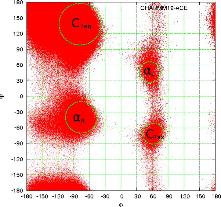
Figure 4: The $\Psi$–$\Phi$ plane for alanine dipeptide. Red dots were obtained from a long brute–force simulation. The initial state is contained in C_7eq and the target state is C_7ax as indicated by the circles. Also shown via circles are the right– and left–handed helical regions, $\mathrm{\alpha_{R}}$ and $\mathrm{\alpha_{L}}$, respectively. Grid lines represent the two–dimensional binning.

For alanine dipeptide in implicit solvent, the configurational space can effectively be condensed to a two–dimensional space given by the $\psi$ and $\phi$ torsional angles. In Figure 4, exploratory brute–force simulations show regions of this two–dimensional configurational space that are populated significantly with a high density of red dots. Also shown in the figure are dashed circles approximately representing states. The region labeled C_7eq contains the starting state (a delta function: $\Phi=-77.9$ and $\Psi=138.4$), and C_7ax is the target state (within a radius of 20 degrees about $\Phi=61.4$ and $\Psi=-71.4$). There are two significant intermediate states – labeled $\mathrm{\alpha_{R}}$ (right–handed helix) and $\mathrm{\alpha_{L}}$ (left–handed helix). The lines show the WE binning in the $\Phi$ and $\Psi$ directions. Note that circularity/periodicity of the $\Phi$ and $\Psi$ angles engenders a multiplicity of pathways between any two states.

An fully atomistic alanine dipeptide molecule using CHARMM 19 forcefield with implicit solvent ACE (analytic continuum electrostatics) model³⁵ is simulated via Langevin dynamics with integration step of 1 fs. The friction constant is set to 50 s^-1. The solvent used is the Analytic Continuum Electrostatics model with the dielectric constant in the region occupied by explicitly modeled atoms as 1 (IEPS parameter), the dielectric constant of space occupied by the solvent as 80 (SEPS parameter), the Gaussian width of density distributions describing volumes of atoms as 1.3 (ALPHA parameter), and the hydrophobic scaling factor, SIGMA, as 3.0. Further, atom–based switching is used.

WE simulations were run as described in Section 2, with the $30^{\circ}\times 30^{\circ}$ bins shown in Figure 4. After the probability adjustment in enhanced WE, the weighted ensemble trajectories are split and combined every 100 fs to keep 20 trajectories in each occupied bin. At these intervals, the trajectories are also analyzed to check if any reach the target state. However, 100 fs interval was determined to be too short for an accurate estimate of the bin populations using eq 2. Thus, for the transition matrix evaluation, the trajectories are checked for transitions every 1000 fs for 500 K, and every 10000 fs for 300 K. Our WE simulation run CHARMM via an in–house C program available to the public.

4 Results

4.1 One–dimensional system

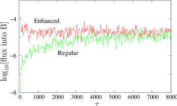
Figure 5: A comparison of fluxes (on log scale) into state B obtained via enhanced (black line) and regular (red line) WE implementation of steady–state procedure for the one–dimensional system of Figure 1. Flux into state B for the one–dimensional system. Due to the probability adjustment procedure, the enhanced version reaches steady state significantly faster. All results shown are window averaged over 100 time increments, $\tau$.

First, we show the correctness of the WE methods and the efficiency gain in the enhanced WE on the one–dimensional energy landscape of Figure 1. The system is challenging because of its high barriers and a deep intermediate state. At steady state, all bins must have time–independent probabilities, and the target state must have a constant probability flux. Figure 5 shows the flux into state B as a function of time obtained using both regular and enhanced steady state procedure of the weighted ensemble path sampling. The two methods agree well - reflecting the fact that the adjustment of initial conditions in the enhanced WE does not affect the steady state solution. Moreover, it shows that the probability adjustment procedure does not disturb the natural system dynamics.

Most importantly, Figure 5 shows that enhanced WE simulation does indeed achieve the steady–state flux value significantly quicker than regular WE. For such a simple system, as used in this example, it is not surprising that the probability adjustment procedure based described above gives a reasonably accurate estimate of the bin probabilities. However, more fundamentally, systems with significant intermediates are not optimally studied via standard WE – nor by, presumably, other methods which fail to “shortcut” intermediate dwell times.

4.2 Two–dimensional system

The two–dimensional systems of Figure 2 and 3 permit us to examine the performance of WE in meeting additional challenges: multiple intermediates, more than one reaction channel, and suboptimal bins.

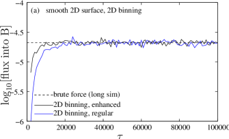
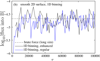
Figure 6: Comparison of WE methods and binning approaches for a smooth two–dimensional potential energy surface. Results from 2D binning are shown in panel (a) and from 1D WE binning are in panel (b). The flux reaches a steady value sooner for the enhanced version than for the regular version. All results agree with each other and also with the final result from long brute–force simulations. All results shown are window averaged using 100 $\tau$ windows.

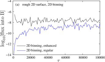
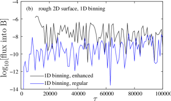
Figure 7: Comparison of WE methods and binning approaches for a rugged two–dimensional potential energy surface. Results from 2D binning are shown in panel (a) and from 1D WE binning are in panel (b). The flux reaches a steady value sooner for the enhanced version than for the regular version. All results agree with each other and also with the final result from long brute–force simulations. All results shown are window averaged using 100 $\tau$ windows.

Again, we first check the correctness of our WE methods for steady state simulation. We plot the fluxes into state B for the smooth and rough two–dimensional potential energy surfaces in Figures 6 and 7, respectively. Each figure show results obtained using both one– and two–dimensional binnings (see Figures 2 and 3). For the less rugged energy landscape, it is possible to obtain accurate brute force results for the mean first passage time, and the inverse of MFPT is the steady state flux into state B. Clearly, this agrees with the steady state flux values obtained using both the enhanced and the regular versions of WE (and with either binning procedure).

One very important observation from Figures 6 and 7 is that the it takes approximately the same amount of time to reach the steady state using enhanced WE simulation, irrespective of the ruggedness of the landscape. However, this is clearly not true for either regular WE or brute–force simulations where the rate decreases by more than three orders of magnitude for the rugged landscape. This again emphasizes the utility of the probability adjustment procedure.

One–dimensional binnings (for both the enhanced and regular WE simulations – red line and the magenta line, respectively) also lead to the correct steady–state flux values into state B. However, the data are noisier. Despite the noisier data, it is clear that the enhanced version reaches the correct steady state flux value faster even for the one–dimensional binning.

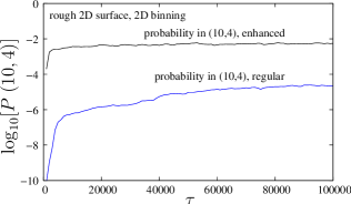
Figure 8: Comparison of WE methods for a single intermediate. Probabilities (log scale) in the bin with indices given by (10,4) are plotted versus time for regular and enhanced WE simulations. The enhanced version reaches a steady value fairly quickly, whereas the regular version does not. All results are window averaged using 100 $\tau$ windows.

Further insight into the discrepancy between regular and enhanced WE simulations for the more rugged landscape is obtained by examining an individual intermediate state. Figure 8 shows the population of a single bin at index (10,4) using both the enhanced (black line) and the regular (blue line) version. Clearly, the enhanced version reaches a plateau value fairly quickly. On the other hand, the population of this bin using regular WE does not reach a plateau value for 10⁵ $\tau$ increments, and is still two orders of magnitude lower than the plateau value of the enhanced version. Thus, Figure 8 clearly illustrates that regular WE attains steady state via regular WE very slowly if there are significant intermediate states.

Efficiency comparison with brute force

To further quantify the gain due to the enhancement procedure, we explicitly compare the efficiency of the enhanced WE approach with the brute–force simulations using the procedure discussed in Section 2.7. For both the potential energy surfaces of Figures 2 and 3, there are three or four intermediate states, depending upon the path. We use $n=3$ for the number of intermediate basins (using another similar number does not qualitatively affect the comparison below). Further, we compare only for the two–dimensional binnings.

For the smoother potential energy surface of Figure 2, the total simulation time required by enhanced WE to reach within one standard error of the steady–state flux is 2$\times 10^{7}\tau$. On the other hand, the estimate for brute–force simulations is 4$\times 10^{5}\tau$. Clearly, for this relatively smooth landscape, brute–force simulations are more efficient than enhanced (and regular) WE.

On the other hand, the converse is obtained for the rougher landscape of Figure 3. Whereas the enhanced WE requires a similar aggregate time to reach the desired deviation from the steady–state flux, the estimate for brute–force simulation balloons to 4$\times 10^{8}\tau$. Thus, with an increase in the roughness of the energy landscape, the enhanced WE progressively outperforms brute–force simulations. This is expected since the time required for brute–force simulations increase in proportion to the MFPT, whereas the enhanced WE requires only a few transition events for the probability adjustment to steady state because WE always finds the transition paths rapidly.

4.3 Alanine dipeptide

Again, for alanine dipeptide, we first demonstrate the correctness of the WE methods by comparing with independent brute–force estimates, and then describe the efficiency gain from the use of enhanced WE. In addition to $T=300$ K, an elevated value (500 K) is studied to permit quantitative comparison with brute–force simulations.

Figure 9 plots the flux into the target state at 500 K using both enhanced and regular versions of WE, along with an independent estimate of flux from brute–force simulations. Both versions give the correct steady state flux values, and these values are obtained in approximately the same number of $\tau$ increments at $T=500$ K.

A similar plot for $T=300$ K is given in Figure 10 (a). As expected, the flux into state B is lower at 300 K compared to 500 K. More importantly, the enhanced version of WE agrees with the brute–force results, however, the flux into state B obtained using the regular version has not reached the correct steady state value in 1400 time increments. Figure 10 (b) further emphasizes the difference between the enhanced and the regular version: the probability in a particular bin with index (4,5) which contains an intermediate state has clearly reached a plateau value in enhanced WE and not in regular WE.

Efficiency comparison with brute force

We compare the efficiency for enhanced WE against brute–force simulations via the method discussed in Section 2.7. Figures 9 and 10 give the steady–state flux and the variance. The gamma distribution model we use has one intermediate basin (i.e., $n=1$). We chose $n=1$ since Figure 4 suggests one intermediate basin along the path from the initial to the final state. However, using other small values of $n$ does not change the qualitative comparison.

We compute the total simulation time using both enhanced WE and brute–force simulations to first attain steady state. At 500 K, the initial phase for rate computation lasts for 10$\tau$ and each $\tau$ during this phase is 1000 fs. This leads to a total simulation time (including all the trajectories) to reach within one standard deviation of the mean steady–state flux using enhanced WE as 60 ns. For $k=1$, brute–force simulations is estimated to require approximately 70 ns. At 300 K, a similar analysis yields an enhanced WE time of 150 ns and a brute–force time of 5 $\mathrm{\mu}$s. Clearly, enhanced WE method is significantly more efficient as the temperature is decreased.

4.4 Equilibrium sampling

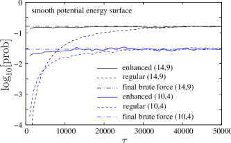
Figure 11: Equilibrium sampling via WE simulation for the smooth two–dimensional potential energy surface. The plot compares probabilities obtained in two different bins (indices (14,9) and (10,4) of Figure 2 (a)) for equilibrium simulations attempted using regular and enhanced WE simulations. Final results from a long brute–force simulation are also shown for reference. The bin probabilities in the enhanced version reach equilibrium values significantly quicker than the regular version.

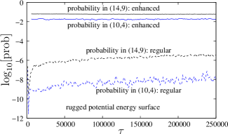
Figure 12: Equilibrium sampling via WE simulation for the rugged two–dimensional potential energy surface. The plot compares probabilities obtained in two different bins (indices (14,9) and (10,4) of Figure 3 (a)) for equilibrium simulations attempted using regular and enhanced WE simulations. The bin probabilities in the enhanced WE simulations reach equilibrium fairly rapidly, whereas the regular WE simulations do not reach equilibrium in the timescale of the simulation.

As mentioned above, the WE steady–state method can easily be adapted to equilibrium sampling, because equilibrium is a steady state. Figure 11 and 12 illustrate WE applied to equilibrium: they shows the populations of two different bins as a function of WE time obtained via enhanced and regular WE simulations for the 2D potential energy surfaces of Figures 2 and 3, respectively. For the smooth potential energy surface, enhanced WE simulation reaches equilibrium in a fairly small number of $\tau$ increments, whereas regular WE requires more time to equilibrate as shown in Figure 11. More dramatically, the regular version does not reach equilibrium in the simulation timescale for the rugged potential energy landscape as shown in Figure 12. On the other hand, even after accounting for an initial time before probability adjustment (equal to $2\times 10^{5}\tau$ for the rugged landscape and only 2000$\tau$ for the smoother one), the enhanced WE remains extremely efficient when compared to regular WE simulations.

Efficiency comparison to brute–force simulations

We now compare the efficiency of enhanced WE to brute–force simulations. From a knowledge of the MFPT for this system, we can also roughly estimate the time required for achieving equilibrium via brute force simulations. We expect equilibrium to be established via brute–force simulations when the brute–force trajectories have traversed the region between the initial and the final state several times. As in Section 4.2, we use the timescale provided by the MFPT and the number of “equivalent” brute–force trajectories ($n=10$, as in Section 4.2) to obtain a rough estimate of the time required for equilibration via brute–force simulations.

For the smoother potential energy surface, $n\times$MFPT equals $5\times 10^{5}\tau$, whereas it equals $4\times 10^{8}\tau$ for the rugged potential energy surface. Establishment of equilibrium via brute–force would require several times these values. On the other hand, enhanced WE simulations require of the order of $5\times 10^{7}\tau$ ($=1000\tau$ for establishment of equilibrium $\times 4500$ trajectories) for establishing equilibrium for the smooth potential energy surface, and approximately $5\times 10^{8}\tau$ for establishing equilibrium for the rugged energy landscape. Thus, the enhanced WE simulation becomes more efficient in establishing equilibrium as the potential energy surface becomes more rugged.

5 Discussion

5.1 Comparison with Markov models

The use of eq 1 is clearly reminiscent of Markov models of the configuration space,^{36, 37} and, for an exact Markovian decomposition, the probabilities obtained via eq 1 should be exact. However, the enhancement procedure we use is qualitatively different from these Markovian models in two crucial ways that we discuss below.

First, we use eq 1 only to estimate the steady–state probabilities in order to shorten the relaxation time to the exact steady state. Thus, the final rates that we obtain are exact and completely independent of a Markovian approximation. Second, the paths obtained via the procedure we presented above are continuous – i.e., we generate trajectories that include time spent within a state. In contrast, Markov models focus only on the hopping between Markovian states.

Despite our approach not relying on Markov models, the efficiency of our probability adjustment protocol for enhanced WE improves significantly by considerations relevant to the Markov models. To elaborate, we recall that the continuous–time trajectories mandate that the rates, $k_{ij}$, used in eq 1 be computed only after a certain relaxation time within a bin for the Markovian picture to emerge.²⁷ Accordingly, the estimates of steady–state probabilities using eq 1 improve if the rates between bins are computed after the relevant intrabin relaxation time.

5.2 Comparing enhanced and regular WE simulation

The main reason for the efficiency gain obtained via enhanced WE as compared to regular WE is that the enhanced WE inherently utilizes the timescale inherent in “fast” trajectories to perform the probability adjustment. In any stochastic process obeying the Fokker–Planck picture (and WE clearly does that²⁶), there is a distribution of transition times from the starting to the target state. Although the nature of this distribution depends upon the exact landscape, the “fast” transitions occur earlier than the mean transition time. The rates between all pairs of bins are computed fairly quickly after the fast trajectories reach the final state, and the probability adjustment procedure of enhanced WE is applied. On the other hand, regular WE must be applied for a time of the order of MFPT to approach steady state.

Due to the wait time for the probability adjustment procedure being of the order of the time it takes the fast trajectories to reach the target state, the efficiency gain for to enhanced WE as the energy landscape becomes more rugged becomes more pronounced (as is clear from a comparison of Figures 6 and 7). The time it takes for the fast trajectories to reach the target state is affected less than the MFPT as the ruggedness of the landscape increases.

5.3 Possible improvements

In this section, we discuss several possible ways to improve the efficiency of the enhanced WE further.

One main avenue for improvement is the construction of better bins between initial and target states. As discussed in Section 5.1, the relaxation time after probability adjustment is minimized if the adjustment procedure results in each bin displaying its steady–state probability. Such optimal bins may be constructed from initial paths or fast trajectories between the starting and the target state. Further, construction of smaller bins reduce the likelihood of significant transverse relaxation within a bin – resulting in a better estimate of steady–state bin probabilities using eq 1.

Even with somewhat suboptimal bins, it is possible to reduce the relaxation time to steady state after probability adjustment by appropriate choice of the number of trajectories in each bin. Currently, all the bins are constructed to have the same number of trajectories – this may not be most efficient for relaxation to steady state after adjustment of probabilities. Bins that are assigned a high population by the probability adjustment procedure but show a subsequent slow decrease in the bin population (due to small rates to other bins) are likely to show a faster relaxation upon an increase in the number of particles. Thus, if the number of particles in each bin is adjusted based on the rate calculation and the assigned probability, the relaxation to steady state may be significantly increased in the enhanced WE.

Another possible strategy for improvement is the use of multiple probability adjustment. As discussed in Section 2.5, only if $\tau$ is longer than intrabin relaxation time that an appropriate estimate of the interbin rates are obtained: the distribution of trajectories within a bin reaches the appropriate steady–state distribution only after the relaxation time. This relaxation time depends on the initial distribution of trajectories, and is minimized as that distribution approaches steady–state values. Accordingly, subsequent instances of rate computation start from trajectories in a bin that are increasingly closer to the steady–state distribution. In this manner, progressively smaller $\tau$ can be used for each probability adjustment segment – thus, improving probability estimates for a given simulation time.

Further improvement is possible if the WE script is fully integrated with the code for underlying dynamics. Currently, the overdamped Langevin dynamics code for the toy models is “hardwired” into the WE code, however, the WE script calls the Langevin dynamics in CHARMM for alanine dipeptide for each trajectory at the beginning of each $\tau$ increment. This results in a significant overhead associated with reinitialization of the underlying CHARMM code in each instance. Due to this, an increase in the magnitude of each $\tau$ does not scale linearly with the wallclock time for alanine dipeptide, whereas this is a linear scaling in the toy models. For example, an increase in $\tau$ from 100 fs to 1000 fs increases the wallclock time by a factor of two for alanine dipeptide for WE simulations.

6 Conclusions

We developed a steady–state path sampling procedure using the weighted ensemble (WE) path sampling method. This procedure does not depend on Markovian decomposition of the configuration space and generated continuous paths from the starting to the final state. The steady state is established via a fairly simple extension of the standard WE path sampling method – a feedback loop into the starting state. The ordinary rate (inverse mean–first–passage time) can also be calculated. A simple probability adjustment procedure, the enhanced WE method, leads to a significantly more efficient attainment of steady state. With an increase in the ruggedness of the energy landscape, the enhanced WE method becomes more efficient as compared to both regular WE and brute–force simulations.

With minor changes to the probability adjustment procedure, the enhanced WE method is applicable for systems at equilibrium, and the probability adjustment allows for a rapid equilibration. We also suggest several possible improvements using optimal bins and number of trajectories within a bin determined from initial paths, as well as by hardwiring the weighted ensemble method into the underlying dynamics code.

Appendix: Potential energies for toy systems

One–dimensional system

The one–dimensional potential is constructed from six half wells glued together from complementary pairs given by

$$U(x)=\frac{3h}{w^{2}}x^{2}\pm\frac{2h}{w^{3}}x^{3}$$ (5)

where $h$ is the depth of each half well and $w$ is the (half) width. The complementary pairs are given by the plus and the minus signs that are valid in the $-w<x<0$ and $0<x<w$ ranges, respectively. Such a potential leads to a smooth potential energy function. In this work, $h=6k_{\mathrm{B}}T$ and $w=1$ m, and the minima are at 1 m, 3 m, and 5 m. The steep repulsions at $x<0$ and $x>6$ are modeled by a $x^{12}$ potential, joined such that the potential energy function remains smooth.

Two–dimensional system

The two–dimensional potential energy function is constructed by the use of laying several energy wells on a flat surface. These energy wells are of the following form:

$$U(r)=-\left(\frac{2h}{w^{2}}r^{2}-\frac{h}{w^{4}}r^{4}\right)$$ (6)

where $h$ and $w$ are the depth and the half width of the wells, respectively. A negative value of $h$ indicates a minimum on the surface, whereas a positive value indicates a maximum. All wells width $w=0.5$ m.

Table 1 gives the values of $h$ used for generating the smooth potential energy surface of Figure 2 for different values of $x$ and $y$. Further, for $|x|>4.0$ or $|y|>4.0$, a repulsive potential of the form: $100(x-4.0)^{2}$$kT$ is used (this is for $x>4.0$, and similar, forms are used for other regions with absolute coordinate greater than 4.0).

The rugged potential energy surface of Figure 3 uses the same form, and has the same values of $w$ as above. The difference is in the values of $h$. For this rugged potential, all positive values of $h$ are replaced by 10 $k_{\mathrm{B}}T$, and all negative values of $h$ become $-5k_{\mathrm{B}}T$, except the one at (-3.5,-0.5) for which $h=-8k_{\mathrm{B}}T$.

Figure 1: Potential energy profile for the one–dimensional system. State B (target state) is defined by $x>4.5$, and state A (initial state) is defined as $0.98<x<1.17$.

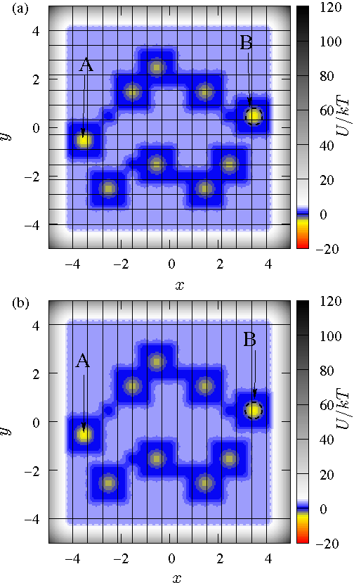
Figure 2: A relatively smooth two–dimensional landscape with two “channels” for transitions from A to B. Two different binning schemes used in WE simulations are shown: (a) two dimensional (b) one dimensional.

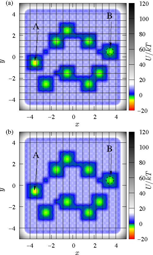
Figure 3: A relatively rugged two–dimensional landscape with two “channels” for transitions from A to B. Two different binning schemes used in WE simulations are shown: (a) two dimensional (b) one dimensional.

Figure 9: Rate estimation for alanine dipeptide at 500 K. The flux into the C_7ax is plotted based on the enhanced WE, regular WE, and final results from long brute–force simulations. All results converge to the same final value, and the enhanced WE is not more efficient than regular WE simulation at this elevated temperature. All results are window averaged using 50 $\tau$ windows.

Figure 10: Comparison of enhanced and regular WE methods for alanine dipeptide at 300 K. The steady state flux into the C_7ax state via the two WE methods and brute–force simulations is shown in panel (a), and the probability in the bin (4,5) in the $\alpha_{\mathrm{R}}$ intermediate state is shown in panel (b). Both panels (a) and (b) show that the regular WE simulation is unable to reach steady state, whereas steady state is established rapidly with the enhanced WE method. All results are window averaged using 50 $\tau$ windows.

Table 1: Well depths, $h$, in units of $k_{\mathrm{B}}T$ for the smooth potential energy surface. Negative values indicate minima on the surface, whereas positive values indicate maxima.

	-4	-3.5	-3	-2.5	-2	-1.5	-1	-0.5	0	0.5	1	1.5	2	2.5	3	3.5	4
-4	3	3	3	3	3	3	3	3	3	3	3	3	3	3	3	3	3
-3.5	3	3	3	3	3	3	3	3	3	3	3	3	3	3	3	3	3
-3	3	3	0	0	0	3	3	3	3	3	0	0	0	3	3	3	3
-2.5	3	3	0	-3	0	3	3	3	3	3	0	-3	0	3	3	3	3
-2	3	3	0	0	0	3	0	0	0	0	0	0	0	0	0	3	3
-1.5	3	3	3	3	3	0	0	-3	0	3	3	3	0	-3	0	3	3
-1	0	0	0	3	3	3	0	0	0	3	3	3	0	0	0	3	3
-0.5	0	-5	0	3	3	3	3	3	3	3	3	3	3	3	3	3	3
0	0	0	0	3	3	3	3	3	3	3	3	3	3	3	0	0	0
0.5	3	3	3	0	3	3	3	3	3	3	3	3	3	0	0	-5	0
1	3	3	3	3	0	0	0	3	3	3	0	0	0	3	0	0	0
1.5	3	3	3	3	0	-3	0	3	3	3	0	-3	0	3	3	3	3
2	3	3	3	3	0	0	0	0	0	0	0	0	0	3	3	3	3
2.5	3	3	3	3	3	3	0	-3	0	3	3	3	3	3	3	3	3
3	3	3	3	3	3	3	0	0	0	3	3	3	3	3	3	3	3
3.5	3	3	3	3	3	3	3	3	3	3	3	3	3	3	3	3	3
4	3	3	3	3	3	3	3	3	3	3	3	3	3	3	3	3	3

References

- 1 B. Alberts et al., Molecular Biology of the cell, Garland Science, New York, 2002.
- 2 A. Fersht, Structure and Mechanism in Protein Science, W. H. Freeman, New York, 2002.
- 3 R. Phillips, J. Kondev, and J. Theriot, Physical Biology of the Cell, Garland Science, New York, 2009.
- 4 T. L. Hill, Free Energy Transduction and Biochemical Cycle Kinetics, Dover Publications, New York, 1989.
- 5 D. Bhatt and D. Zuckerman, http://arxiv.org/abs/1002.2402 (2010).
- 6 L. R. Pratt, J. Chem. Phys. 85, 5045 (1986).
- 7 C. Dellago, P. G. Bolhuis, F. S. Csajka, and D. Chandler, J. Chem. Phys. 108, 1964 (1998).
- 8 C. Dellago, P. G. Bolhuis, and D. Chandler, J. Chem. Phys. 110, 6617 (1999).
- 9 P. G. Bolhuis, D. Chandler, C. Dellago, and P. L. Geissler, Annu. Rev. Phys. Chem 53, 291 (2002).
- 10 T. S. van Erp, D. Moroni, and P. G. Bolhuis, J. Chem. Phys. 118, 7762 (2003).
- 11 T. S. van Erp and P. G. Bolhuis, J. Comp. Phys. 205, 157 (2005).
- 12 T. S. van Erp, Comp. Phys. Commun. 179, 34 (2008).
- 13 R. J. Allen, P. B. Warren, and P. R. ten Wolde, Phys. Rev. Lett 94, 018104 (2005).
- 14 R. J. Allen, D. Frenkel, and P. R. ten Wolde, J. Chem. Phys. 124, 024102 (2006).
- 15 R. J. Allen, D. Frenkel, and P. R. ten Wolde, J. Chem. Phys. 124, 194111 (2006).
- 16 C. Valeriani, R. J. Allen, M. J. Morellia, D. Frenkel, and P. R. ten Wolde, J. Chem. Phys. 127, 114109 (2007).
- 17 E. E. Borrero and F. A. Escobedo, J. Chem. Phys. 127, 164101 (2007).
- 18 A. K. Faradjian and R. Elber, J. Chem. Phys. 120, 10880 (2004).
- 19 A. M. A. West, R. Elber, and D. Shalloway, J. Chem. Phys. 126, 145104 (2007).
- 20 A. Warmflash, P. Bhimalapuram, and A. R. Dinner, J. Chem. Phys. 127, 154112 (2007).
- 21 A. Dickson, A. Warmflash, and A. R. Dinner, J. Chem. Phys. 130, 074104 (2009).
- 22 W. vanden Eijnden and M. Venturoli, J. Chem. Phys. 131, 044120 (2009).
- 23 G. A. Huber and S. Kim, Biophys. J. 70, 97 (1996).
- 24 E. W. Fisher, A. Rojnuckarin, and S. Kim, J. Molec. Struct.–Themochem 529, 183 (2000).
- 25 B. W. Zhang, D. Jasnow, and D. M. Zuckerman, Proc. Natl. Acad. Sci. 104, 18043 (2007).
- 26 B. W. Zhang, D. Jasnow, and D. M. Zuckerman, J. Chem. Phys. 132, 054107 (2010).
- 27 N.-V. Buchete and G. Hummer, Phys. Rev. E 77, 030902 (2008).
- 28 X. Huang, G. R. Bowman, S. Bacallado, and V. S. Pande, Proc. Natl. Acad. Sci. 106, 19765 (2009).
- 29 H. Flyvbjerg and h. G. Petersen, J. Chem. Phys. 91, 461 (1989).
- 30 R. V. Hogg and A. T. Craig, Introduction to Mathematical Statistics, Macmillan, New York, 1978.
- 31 T. B. Woolf, Chem. Phys. Lett. 289, 433 (1998).
- 32 A. van der Vaart and M. Karplus, J. Chem. Phys. 126, 164106 (2007).
- 33 H. Jang and T. B. Woolf, J. Comput. Chem. 27, 1136 (2006).
- 34 W. Ren, E. vanden Eijnden, P. Maragakis, and E. Weinan, J. Chem. Phys. 123, 134109 (2005).
- 35 M. Schaefer and M. Karplus, J. Phys. Chem. 100, 1578 (1996).
- 36 D. J. Wales, J. Chem. Phys. 130, 204111 (2009).
- 37 J. D. Chodera, N. Singhal, W. C. Swope, V. S. Pande, and K. A. Dill, J. Chem. Phys. 126, 155101 (2007).