IRAS 16293: A “Magnetic” Tale of Two Cores

Abstract

We present polarization observations of the dust continuum emission from the young star forming region IRAS 16293. These observations of IRAS 16293, which is a binary system, were conducted by the Submillimeter Array (SMA) at an observing frequency of 341.5 GHz ($\lambda\sim 880\mu$m) and with high angular resolution ($\sim$2$\arcsec$–3$\arcsec$). We find that the large scale global direction of the field, which is perpendicular to the observed polarization, appears to be along the dust ridge where the emission peaks. On smaller scales we find that the field structure is significantly different for the two components of the binary. The first component, source A, shows a magnetic field structure which is “hourglass” shaped as predicted from theoretical models of low mass star formation in the presence of strong magnetic fields. However, the other component, source B, shows a relatively ordered magnetic field with no evidence of any deformation. We have possibly detected a third younger outflow from source A as seen in the SiO emission which is in addition to the two well known powerful bipolar outflows in this kinematically active region. There is an observed decrease in polarization towards the center and this “polarization hole” is similar to decreases seen in other young star forming regions. Our calculations show that in IRAS 16293 the magnetic energy is stronger than the turbulent energy but is approximately similar to the centrifugal energy. There is considerable misalignment between the outflow direction and the magnetic field axis and this is roughly in agreement with model predictions where the magnetic energy is comparable to the centrifugal energy. In conjunction with other observations of the kinematics as determined from the outflow energetics and chemical differentiation we find that our results provide additional evidence to show that the two protostars appear to be in different stages during their evolution.

1 Introduction

In the “classical picture” of star formation, magnetic fields are believed to strongly influence star formation activity in molecular clouds. They provide support to a cloud against gravitational collapse and thus explain the low efficiency of the star formation process (Mouschovias, 2001; Shu et al., 2007). The process of ambipolar diffusion, in which magnetic flux is redistributed in the cloud, leads to the formation of a core that can no longer be magnetically supported and gravitational collapse sets in. In addition, the process of magnetic braking can help to remove angular momentum and slow down the rotation of the cloud as it collapses (Basu & Mouschovias, 1994). In contrast, there have been a number of alternate theories which postulate that magnetic fields are relatively weak and supersonic magnetohydrodynamic turbulence is the dominant process (Mac Low & Klessen, 2004). Turbulence controls the evolutions of clouds, and cores form at the intersection of supersonic turbulent flows. Only a fraction of such cores become supercritical and collapse begins to occur on a gravitational free-fall timescale (Ballesteros-Paredes et al., 2007).

Studying the morphology of the magnetic field in the interstellar medium (ISM) requires difficult and sensitive observations of polarized radiation (Hildebrand & Kirby, 2004). Spinning dust grains in the ISM become partially aligned with the magnetic field, generally with their long axes perpendicular to the field (Davis & Greenstein, 1951). Nevertheless, the exact nature of the alignment process is a matter of debate (Lazarian, 2007), but it appears that the dominant mechanism may actually be alignment by radiative torques (Hoang & Lazarian, 2008, 2009). As a consequence of this alignment, the thermal dust emission is partially linearly polarized, with polarization direction perpendicular to the magnetic field. The magnitude of the field can be determined indirectly by using the dispersion of the position angles of the field under the assumption of energy equipartition between the kinetic and perturbed magnetic energies (Chandrasekhar & Fermi, 1953; Ostriker et al., 2001; Heitsch et al., 2001; Crutcher et al., 2004; Falceta-Gonçalves et al., 2008).

Observations of the large scale polarization distribution in molecular clouds from optical, infra-red, and submillimeter (submm) wavelengths usually show an ordered pattern (Dotson et al., 2000; Pereyra & Magalhães, 2004; Poidevin & Bastien, 2006; Matthews et al., 2009). The analysis of polarization data has showed that some dark clouds are magnetically dominated (Alves et al., 2008; Heyer et al., 2008) while other giant molecular clouds are close to equipartition with turbulence (Novak et al., 2009). However, observationally, the debate on whether turbulence or magnetic fields are dominant is still unresolved (Crutcher et al., 2009). Early and pioneering work with the BIMA millimeter (mm) array showed the dust (and molecular line) polarized emission can be traced at an angular resolution of few arcseconds, the scales where the core contraction process occurs (Rao et al., 1998; Girart et al., 1999; Lai et al., 2001, 2003; Cortes et al., 2005). Currently, the Submillimeter Array (SMA) is the only telescope that can detected the polarized emission at mm and submm wavelengths (Marrone et al., 2006; Girart et al., 2006, 2009; Tang et al., 2009a, b). In the object NGC 1333 IRAS 4A (IRAS 4A here after), the SMA observations have revealed that the magnetic field configuration is consistent with theoretical models for the formation of solar-type stars in which magnetic fields play a much stronger role than turbulence (Girart et al., 2006; Gonçalves et al., 2008).

The low-mass star forming region IRAS $16293-2422$ (IRAS 16293 here after), located in the $\rho$ Ophiuchi molecular cloud complex, has been the focus of numerous studies since the report of infall spectral signatures (Walker et al., 1986; Menten et al., 1987). Accurate observations using astrometric techniques show that the $\rho$ Ophiuchi molecular cloud is at a distance $\simeq 120$ pc (Knude & Hog, 1998; Loinard et al., 2008), while maser VLBI observations towards IRAS 16293 suggest a distance of $\simeq 178$ pc (Imai et al., 2007). For this paper we have assumed a distance of $d=150$ pc. IRAS 16293 is a Class 0 protostellar system with a bolometric luminosity of 32 L_☉, and is surrounded by a compact, $R_{\rm env}\simeq 3000$ AU, but relatively massive envelope, $\simeq 3.0$ M_☉, (Correia et al., 2004). Higher resolution radio interferometric observations have revealed a double core separated by 5$\arcsec$ (750 AU in the plane of the sky). The southern core is commonly referred to as source A and the northern one as source B. Both cores appear to have different physical and chemical properties (Wootten, 1989; Estalella et al., 1991; Bottinelli et al., 2004; Chandler et al., 2005; Takakuwa et al., 2007). Despite its low luminosity, IRAS 16293 has a rich chemistry, with hot-core like properties at scales of $\sim 100$ AU (Blake et al., 1994; Ceccarelli et al., 2000; Schöier et al., 2002; Cazaux et al., 2003; Kuan et al., 2004; Bisschop et al., 2008). There is a strong quadrupolar outflow associated with source A (Walker et al., 1988; Mizuno et al., 1990; Stark et al., 2004; Yeh et al., 2008). The larger bipolar outflow is in the east-west direction (E-W outflow), with a position angle (PA) of $110\arcdeg$. The other outflow is in the northeast-southwest direction (NE-SW outflow), with a PA of $60\arcdeg$ and shows copious SiO emission (Hirano et al., 2001). High resolution submm observations (Chandler et al., 2005) have revealed multiplicity in source A and which of these sources powering these two outflows is a matter of debate (Loinard et al., 2007). Previous measurements of the magnetic field geometry in this object by observing polarized dust emission have yielded contradictory results (Flett & Murray, 1991; Tamura et al., 1993; Akeson & Carlstrom, 1997), possibly because they were sensitivity limited. Thus, it is apparent that more sensitive and higher resolution observations of the magnetic field structure are needed.

In § 2 we briefly describe the observations and the data reduction procedure. § 3 presents the results, § 4 the analysis, and § 5 discusses the possible scenarios for the observed magnetic field morphology in context with the information from observations already known from the literature.

2 Observations and Data Analysis

The observations were conducted in April 2006 (see details in Table 1) with the SMA, which is located near the summit of Mauna Kea in Hawaii (Ho et al., 2004). As can be seen from the Caltech Submillimeter Observatory (CSO) tau meter atmospheric opacities in Table 1, the observing conditions on the first day were significantly better than those on the second day. Nevertheless, the atmospheric conditions were stable on both days resulting in minimal fluctuations in the antenna gains. The coordinates of the pointing center was at RA=$16^{h}32^{m}22\fs 9$ and Dec.=$-24\arcdeg 28\arcmin 36\farcs 00$. The observing frequency was chosen to be located in the 345 GHz atmospheric window, which at the Mauna Kea site provides both optimal sensitivity and angular resolution. The SMA receivers operate in a double sideband mode with the two sidebands separated by $\sim$10 GHz and the selected local oscillator frequency placed the lower and upper sideband central frequencies at 336.5 GHz and 346.5 GHz respectively. The SMA correlator has a bandwidth of $\sim$2 GHz which comprises of 24 partially overlapping spectral windows. All the spectral windows had 128 channels, which provided a velocity resolution of 0.7 km s^-1. In addition to the continuum, the tuning frequency and the correlator were chosen to allow for simultaneous observation of the emission from the CO 3–2, SiO 8–7, and H¹³CO⁺ 4–3 spectral lines.

Conducting polarimetric observations with interferometer arrays at mm and submm wavelengths is challenging and requires the use of some special techniques. A brief description of these techniques is provided in Marrone et al. (2006) and a more detailed discussion of the methodology (both hardware and software aspects) is available in Marrone (2006) and Marrone & Rao (2008). The data were reduced using the MIRIAD software package (Wright & Sault, 1993). The instrumental gains were calibrated by interspersing observations of IRAS 16293 (the target source) with observations of the quasars J$1517-243$ and J$1622-297$ which were used as gain calibrators. The instrumental spectral bandpass was calibrated from observations of the quasar 3C 273 and the absolute flux scale was determined from observations of Callisto. The single greatest factor that can corrupt the data is the intrinsic instrumental polarization which is commonly referred to as the “leakage”. Therefore, the data were needed to be carefully calibrated to remove the effects due to this leakage. The primary task in MIRIAD which was used to solve for the leakage is GPCAL. For our observations we used 3C 273, whose intensity and polarization are strongly variable. In addition to the leakage, the task GPCAL also simultaneously solves for the polarization of the calibrator as well. At the epoch of our observation, we determined the intensity to be $\sim$8.7 Jy and the linear polarization to be $1.0\pm 0.1$% at a position angle of $-34\arcdeg$. The leakages are different in each of the two sidebands as they differ in frequency by $\sim$10 GHz. In the upper sideband, which is closer to the design frequency of the SMA polarimetry system, the measured leakages were approximately 1%, while the lower sideband leakages were between 2 and 3%. These leakages were measured to an accuracy of 0.2% or better.

The data from the source of interest, IRAS 16293, were then corrected for the leakages. The continuum emission in each of the two sidebands is contaminated by the emission from various spectral lines. The strongest spectral line emission that we detect is the one from the CO 3–2 transition located at a rest frequency of 345.796 GHz. In addition, there is spectral line emission from various molecules such as SiO (8–7 transition) and H¹³CO⁺ (4–3 transition), as well as SO₂ and CH₃OH. There was also emission from other molecular transitions, but these were significantly weaker. The CO and SiO spectral lines are good tracers of the outflow activity in the earliest stages of star formation, whereas the H¹³CO⁺ is a good tracer of the dense circumstellar gas. To create a pseudo-continuum channel for each sideband the contribution from the spectral lines was removed and the data were then averaged over all the spectral channels. These spectral line free and polarization calibrated data were used to produce maps of the I, Q, and U Stokes parameters. These maps were then independently deconvolved using the CLEAN algorithm. Since the continuum emission (Stokes I) from this source is quite strong, the source visibilities could be self-calibrated. The gain solutions from the self-calibration were applied to all the Stokes visibilities (continuum and line emission). The Q and U maps were combined to produce maps of the debiased linear polarization intensity (Leahy & Fernini, 1989), the fractional polarization, and the position angle. Continuum maps were made in each sideband separately for each of the observing dates and these were identical within the limits of the noise. Combined maps were then obtained using with the two sidebands and the two observing dates. Stokes I, Q and U maps of CO 3–2, SiO 8–7, and H¹³CO⁺ 4–3 were also obtained. For the spectral lines, we present only the Stokes I line emission, since no significant polarized line emission was detected. Table 2 lists the basic parameters of the resulting maps, including the frequency of the spectral lines or continuum, the channel resolution (for line observations), the resulting synthesized beam, and the root mean square ($rms$) noise of the maps.

3 Results

3.1 Continuum Emission

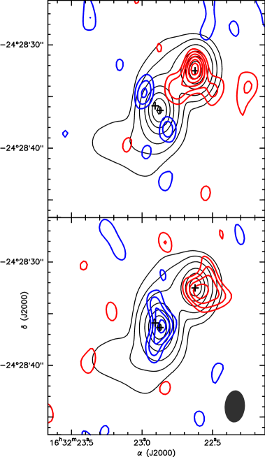
Figure 1: Top panel: Color contour map of the Stokes U dust emission overlaid on the black contour map of the total dust emission (Stokes I). Stokes U blue (negative) and red (positive) contours are $-5$, $-4$, $-3$, $-2$, 2, 3, 4, 5, 6, and 7 times the $rms$ noise of the map, 4 mJy beam^-1. Stokes I contours are 2, 7, 17, 37, 57, 77, and 97% of the peak intensity (4.1 Jy beam^-1). Crosses mark the position of Aa, Ab, and B sources (Loinard et al., 2007). The synthesized beam is shown in the bottom right. Bottom panel: Same as previous panels, but with Stokes Q in blue (negative) and red (positive) contours.

The Stokes I map of the total continuum flux density is shown in Figure 1. The continuum emission, which arises from the warm dust, is quite strong and is resolved into the two well known components, sources A & B (Wootten, 1989). Subarcsecond resolution observations at $\lambda\sim 1$ mm show that source A itself is comprised of two components, Aa and Ab, separated by 0.6$\arcsec$ (Chandler et al., 2005) with Aa located southwest of Ab. In addition, subarcsecond VLA observations show that the centimeter (cm) wavelength emission from Aa can be further split into two additional components (Loinard et al., 2007). The peak of the Stokes I continuum is $\sim 4.1$ and $\sim 3.9$ Jy beam^-1 for source A and B respectively, and the integrated flux from both sources is approximately 11.5 Jy. The absolute flux scale at the SMA is only determined to an accuracy of 5% and thus all the flux densities calculated by us are uncertain by this factor. Single dish observations with the JCMT at 850 $\mu$m ($14\farcs 6$ beam) measure a flux of $23.6\pm 1.3$ Jy within a radius of $20\arcsec$ of the two sources (Correia et al., 2004). The SMA measurements appear to detect about half of the total flux. This is due to the fact that the SMA antennas have a primary beam size (diameter) of 34$\arcsec$ at the chosen observing frequency and the sensitivity to extended structure degrades as the distance from the pointing center increases. This missing undetected flux must therefore arise from emission on size scales larger than $\sim 15\arcsec$ which is about six times the synthesized beam size.

A Gaussian fit to source B shows that is barely resolved (see Table 3), with a radius less than 100 AU. This is consistent with previous higher angular resolution observations which indicate that the dust emission comes from a optically thick disk with an outer radius of 26 AU (Rodríguez et al., 2005; Loinard et al., 2007). The measured flux of source B is in agreement with the value measured at at frequency of 305 GHz by Chandler et al. (2005) with higher angular resolution, after taking into account its spectral index. The Gaussian fit to source A shows that this source is more extended, and is resolved with a deconvolved scale of $330\times 180$ AU, elongated in the north-south direction (see Table 3). The flux measured is $\sim 1$ Jy higher than that expected from Chandler et al. (2005), probably because they filter some emission in their higher angular resolution maps. In addition to the contribution from sources A and B, there is some contribution from more extended dust, mostly from the southeastern part of source A and also north of source A (east of source B). The total flux measured with the two Gaussian fits of is $\simeq 10.6$ Jy (Table 3), whereas the total flux measured with the SMA is 11.5 Jy.

3.2 Dust Polarization

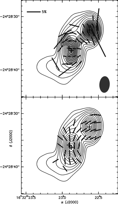
Figure 2: Top panel: Contour map of the total (Stokes I) dust emission overlaid on the grayscale image of the polarized dust intensity. The gray bars represent the polarization vectors. The 5% vector length is shown in the top left panel for comparison. Their length is proportional to the polarization fraction. Contours are 2, 4, 7, 11, 18, 28, 38, 48, 58, 68, 78, 88, and 98 percent of the peak intensity (4.1 Jy beam^-1). Black crosses mark the position of Aa, Ab, and B sources (Loinard et al., 2007). The synthesized beam is shown in the bottom right. Bottom panel: Contour map of the total dust emission as in the top panel. The bars represent the magnetic field vectors.

The linearly polarized component of the emission can be obtained from maps of Stokes Q and U. Typically, this is quite small and is only a few percent of the Stokes I emission. The maps for Stokes Q and U are plotted in in the top and bottom panels of Figure 1. The peak (absolute) values of Stokes Q and U are $\sim$ 7 times the noise level of $\sim$ 4 mJy beam^-1. Note that in contrast to Stokes I which is a positive quantity, Q and U can be negative. We then obtained the maps of the (debiased) linearly polarized flux density ($P$), the polarization position angle ($\theta$), and the fractional polarization ($p$) which is expressed as a percentage. The maps of the errors in $P$, $p$, and $\theta$ are obtained as well. The map of the polarized intensity, fractional polarization, and position angle overlaid on a map of the total intensity is shown in the top panel of Figure 2. The fractional polarization and position angle are only computed at points where the debiased polarized flux density is greater than 8 mJy beam^-1 ($\sim 2\sigma$). Table 4 contains a listing of the polarizations measured at various locations on the map. The errors in fractional polarization and position angle depend inversely on the Stokes I flux density and the polarized flux density respectively. Consequently, the errors in the fractional polarizations are smaller in regions where the continuum flux density is higher, while the position angle errors are smaller where the polarized flux density is larger.

From the map of the polarized emission (top panel of Figure 2) we can see that the polarization structures and morphologies are considerably different for the two sources A and B. The position angles of the linear polarization around source A appear to be approximately in a “centrosymmetric” pattern. Such a pattern can also be produced when the polarization is caused due to scattering (Silber et al., 2000). The scattering cross-section of the dust grains is quite significant in the optical and near-IR bands. However, it is inversely proportional to $\lambda^{4}$ and thus the scattered polarized radiation decreases rapidly as the wavelength increases. Therefore, the contribution from scattering is likely to be negligible at the much longer submm observations. The polarization that is observed by us with the SMA must therefore arise largely from the continuum dust emission.

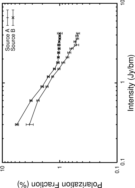
Figure 3: The fractional polarization as a function of total intensity for each of the two sources A and B. The decrease in fractional polarization at large continuum Stokes I (also called a “polarization hole”) has also been seen at other polarization observations as well (Schleuning, 1998). For both sources the errorbars are also plotted and the fractional polarization errors are quite small compared to the value.

The polarization fraction for the emission from source B is higher than that of source A, as seen in Figure 3. Furthermore, this plot shows that the decrease in fractional polarization at larger values of the total intensity is greater for source A. This decrease in fractional polarization towards the center of the cores where the peak emission is higher indicates that there may be a “polarization hole” effect. This decrease or depolarization is also seen in other sources as well (Schleuning, 1998; Matthews et al., 2001; Lai et al., 2002). This effect could be due to at least three possible factors. Firstly, the higher density and temperature towards the center of the sources can lead to a misalignment due to the effects of a higher collisional rate and hence lower the degree of polarization. Secondly, the grain properties towards the center could be different from the grain properties in the outer envelope with the grains in the center being less able to align with the field than the grains in the envelope. The difference in the decreases in sources A and B could possibly be due to differences in the grain growth and properties in the two sources. One other possibility, which our observations seem to hint at, is that this decrease is due to the significant disparity in the morphology of the magnetic field. This central depolarization was also suggested by Matthews et al. (2001) from their observations of the OMC-3 filaments in Orion A. Towards the center of source A, the magnetic field directions change significantly over small scales leading to spatial variability in the position angles of the polarized emission. The resolution of our observations is not sufficient to resolve the small scale structure. This results in lower polarization at the center due to the averaging of small scale structure.

The polarized emission from this source has been the target of a number of different observations conducted both with single dish telescopes and interferometer arrays at a range of wavelengths (Table 5). As mentioned earlier in the introduction, most of the early measurements were inconsistent with each other, which was perhaps due to limited sensitivity. A more recent polarization map from the JCMT using the Submillimeter Common Use Bolometer Array (SCUBA) polarimeter shows that at the peak of the dust continuum emission, no polarization is detected (Matthews et al., 2009). We can compare our observations by convolving our images by the beam equal to the resolution of the JCMT. Since almost all of the area over which the polarized dust emission detected by the SMA is within the JCMT beam, this is approximately equal to the integrated polarization over our map. When this is done we obtain extremely low polarizations around  0.2% (Table 5), and is in good agreement with the SCUBA measurements.

Under the assumption that the grains are not spherical and are rotating about their short axis which is aligned with the magnetic field, the field structure can be obtained by rotating the position angle of the observed polarization by $90\arcdeg$ (bottom panel of Figure 2). There is considerable spatial structure in the deduced magnetic field directions, with a large scale twisted magnetic field in a direction coinciding with a curve joining sources A and B. In addition, source A shows that the lines are deformed with an “hourglass” like structure. This is the second such sensitive detection of this type of “hourglass” structure towards a region of low mass star formation. The first was the young stellar object IRAS 4A reported by Girart et al. (2006). In contrast, source B shows very little variation in magnetic field structure.

3.3 Molecular Lines

3.3.1 H¹³CO⁺  4–3

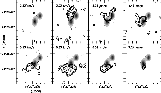
Figure 4: Contour channel maps of the H¹³CO⁺ 4–3 line emission overlaid on the dust emission which is shown in the gray scale. The contour levels are $-3$, 3, 4, 5, 7 and 9 times the $rms$ noise level, 0.42 Jy beam^-1. The $v_{\rm LSR}$ velocity of each channel is shown in the top left corner of the panels.

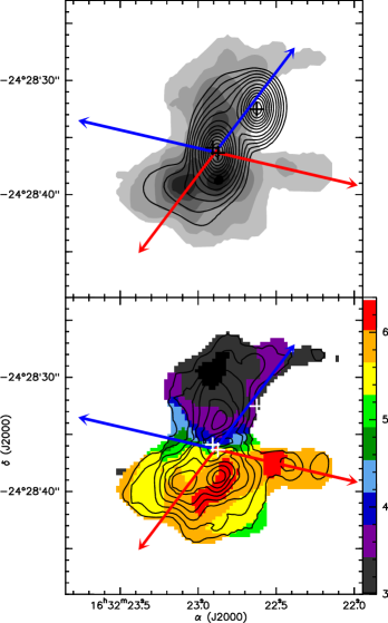
Figure 5: Top panel: Contour maps of the dust emission overlaid with the integrated intensity (zeroth moment) gray scale image of the H¹³CO⁺ 4–3 line emission. Contours levels are the same as those in Fig. 2. Crosses mark the position of Aa, Ab, and B. Blue and red arrows show the directions of the E-W CO outflow and the NW-SE SiO outflow. Bottom panel: Contour maps of the integrated intensity (zeroth moment) overlaid with the intensity weighted velocity (first moment) color image of the H¹³CO⁺ 4–3 line emission. Contour levels go from 5 to 95% the maximum value (8.7 Jy km s^-1) with steps of 15%. The units of the vertical bar is in km s^-1. Crosses mark the position of Aa, Ab, and B.

Figure 4 shows the channel maps of the H¹³CO⁺ 4–3 emission while Figure 5 shows the integrated emission and the velocity field. Both figures show that the H¹³CO⁺ emission arises roughly extended in the north-south direction over approximately $17\arcsec\times 10\arcsec$ ($2500\times 1500$ AU) and centered on source A. The strongest emission is offset by a few arcseconds to the north and south of source A. Indeed, the H¹³CO⁺ integrated emission presents a relative minimum at the position of source A. Source B appears to be devoid of the H¹³CO⁺ emission. As shown in Figures 4 and 5, there are clear signs of a velocity gradient along the major axis of the H¹³CO⁺ structure (north-south direction) of about $\simeq 0.31$ km s^-1 arcsec^-1, which translates to a physical scale of 430 km s^-1 pc^-1, or an angular velocity, $4.5\times 10^{-12}$ s^-1. This is almost one order of magnitude higher that the value found by Narayanan et al. (1998) from single-dish observations of the IRAS 16293 core. It is possible that this discrepancy may be due to the different scales that are being probed. The Narayanan et al. (1998) scale-sizes are $\sim$39$\arcsec$ which is more than twice the maximum structures being mapped by us. The north-south velocity gradient is also observed in the H₂CO $4_{1,3}$–$3_{1,2}$ line, although this line has a slightly different morphology: its emission arises from the two sources, A and B, and it is extended south of source A (Chandler et al., 2005).

3.3.2 SiO  8–7

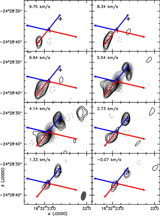
Figure 6: Channel contour maps of the SiO 8-7 line emission. For two of the channels, the dust continuum image in gray scale is overlaid. Contours are $-3$, 3, 4, 5, 7, 9, 11, 13 and 15 times the $rms$ noise level, 0.35 Jy beam^-1. Crosses mark the position of Aa, Ab and B. The directions of the outflow is shown as red and blue arrows. The SE-NW arrows have a position angle of $145\arcdeg$ and are centered on source Ab, and matches well with most of the SiO emission. The NE-SW arrows have a position angle of $105\arcdeg$ and are centered on source Aa.

Figure 6 shows the channel maps of the SiO 8–7 emission, which extends in velocity over 10 km s^-1 and is split into three main condensations. The most prominent one is observed just southeast of source A (SE condensation), and is detected in all the displayed channels, although it is brighter at the redshifted velocities. A Gaussian fit to the emission from this condensation in the $v_{\rm LSR}=6.94$ km s^-1 velocity channel gives a position angle of $145\arcdeg$, which is similar to the overall orientation of this condensation with respect to source A (see Figure 6). The second condensation appears to arise northwest of source A (and southeast of source B) at systemic and blueshifted velocities (NW–1 condensation). At the $v_{\rm LSR}$ of 5.5 km s^-1 the emission appears to break up into two condensations (also partially observed at the 4.14 km s^-1 velocity channel). The peak intensity of the brightest channels appears to be located in the same axis as the one formed between SE condensation and source A. Indeed, the line that connects the SE and NW condensation passes closer to Ab than Aa. The third condensation is located about 6$\arcsec$ northwest of source B (NW–2 condensation).

3.3.3 CO  3–2

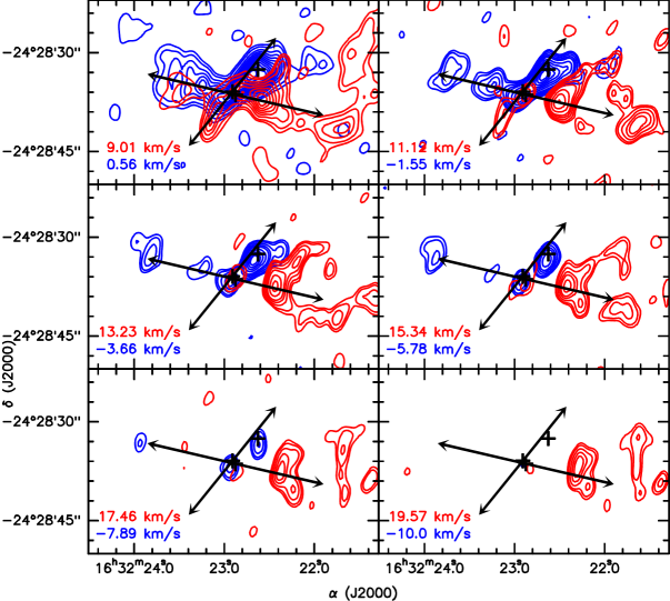
Figure 7: Channel maps of the CO 3-2 for the blueshifted (blue contours) and redshifted (red contours) emission. For the top-left panel the contours are 5, 10, 20, 30, $\dots$ 120 times the $rms$ noise level, 0.25 Jy beam^-1. For the other panels, the contours are 4, 6, 10, 15, 20, 30, 40, 50, 60, 70 and 80 times the $rms$ noise level. The $v_{\rm LSR}$ velocity of each channel is indicated in the top left part of each panel.

The high angular resolution maps of the CO emission (for the 2–1 and 3–2 lines) from SMA observations have been already reported in the literature (Yeh et al., 2008). The emission is quite extended in the east-west direction (E-W outflow). In the visibility domain of our CO 3–2 data set, this shows up as a steep increase of the CO flux for visibilities with a radius, $r_{u,v}$, shorter than 20 k$\lambda$. Figure 7 shows the channel maps of the CO 3–2 obtained by excluding the visibilities with $r_{u,v}<20$ k$\lambda$. The most prominent emission comes from the E-W outflow. The blueshifted eastern lobe is more collimated than the redshifted western lobe, which has an open shell structure. The position of peak intensity of the brightest clumps (both eastern and western) appear to be well aligned, crossing source A, with a PA$\simeq 105\arcdeg$. The SiO outflow is also traced by the CO 3–2 emission. The SiO SE condensation is detected in the lowest redshifted velocity channels ($v_{LSR}=9.0$ and 11.1 km s^-1). There is also blueshifted CO emission apparently associated with the SiO NW 1 condensation, although the emission appears to be slightly displaced to the west, with the emission even being more bent to the west of source B.

4 Analysis

4.1 Distribution of Polarization Position Angles

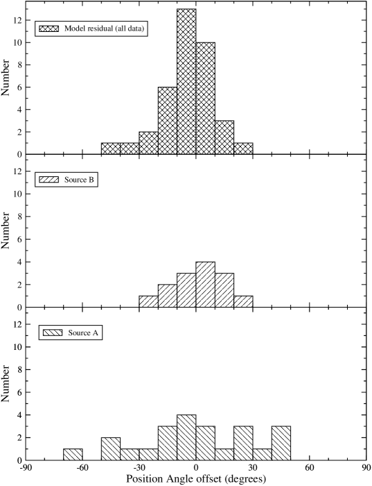
Figure 8: From bottom to top: Position angle (PA) distribution of the polarization vectors around source A with respect to the average value, $<$PA$>=95.0\arcdeg$. PA distribution of the polarization vectors around source B with respect to the average value, $<$PA$>=24.0\arcdeg$. PA distribution of the residual from the parabolic fitting done to the source A data and applied to all the data (i.e. including source B), which is shown in Figure 9.

The average values of the polarization PA around source A and B are $95\arcdeg$ and $24\arcdeg$ respectively. The distribution of the residual values of the polarization PA after subtraction of the average values around source A and B are shown in the bottom panel and the middle panel of Figure 8 respectively. This distribution shows that source B has a more uniform pattern than source A, which is likely due to the deformed morphology in the east-west direction (see Figure 2). In spite of the magnetic field structure, the analysis of the dispersion of the position angle as a function of displacement through the “structure function” can provide an indirect measurement of the turbulent to magnetic energy ratio (Hildebrand et al., 2009). Since the range of scales where the polarization is detected is small, we prefer to fit the magnetic field morphology around source A in a similar way as was done in IRAS 4A (Girart et al., 2006). As a first approximation of the field geometry we fit the magnetic field vectors around source A only, excluding those around source B, with a set of parabolas. The results obtained with this method are in fair agreement with a more detailed analysis using specific theoretical magnetic field geometries (Gonçalves et al., 2008). The parabolic functions used are of the type:

$$(y-y_{0})=g_{i}+g_{i}\,C(x-x_{0})^{2}$$ (1)

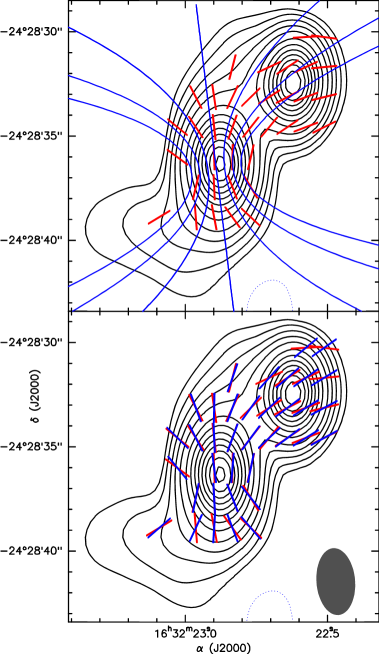
Figure 9: Top panel: Overlap of the 0.88 mm dust emission and the B-vectors (same as Figure 2) with the best solution for the parabolic family of functions (blue solid lines). Bottom panel: Same as top panel, but the best family of functions are shown as B-vectors (in blue) at the same position as the measured values.

where $y_{0}$ and $x_{0}$ is the center of symmetry of the magnetic field configuration. The quantity $g_{i}$ is a parameter which depends on the curve that is selected and $g_{i}C$ represents the quadratic term. Note that the main magnetic field direction is along the $x$ axis, and that for the observed magnetic field morphology, the $y$ axis is going to be close to the right ascension axis. We used the $\chi^{2}$ method with $y_{0}$, $x_{0}$, $C$ and the position angle of the main direction of the magnetic field, $\theta_{\rm B}$ as free parameters. The best fit solution obtained is with $x_{0}=-0\farcs 10$, $y_{0}=-0\farcs 62$, $C=0.25$ and $\theta_{\rm B}=7.0\arcdeg$. Figure 9 shows the best solution for five sets of parabolas (top panel), and the values of the modeled magnetic vectors at the position of the observed magnetic field vectors (bottom panel). It is remarkable that this solution not only fits the magnetic field vectors around source A, but those around source B as well even though these were not used in the fitting! The distribution of the residuals, including the magnetic field vectors from source B, is shown in the top panel of Figure 8. The standard deviation of the residuals is $\delta\theta_{obs}=13.9\arcdeg\pm 0.6\arcdeg$. The uncertainty of the polarization position angle is $\sigma_{\theta}=9.8\arcdeg\pm 3.8\arcdeg$, so the intrinsic dispersion is $\delta\theta_{\rm int}=9.8\arcdeg\pm 3.9\arcdeg$.

4.2 Physical Parameters: Mass, Density and Column Density

We can infer the total mass from the intensity of the dust emission using the following relation (Hildebrand 1983)

$$M=\frac{Fd^{2}}{\kappa B(T)}$$ (2)

where $F$ is the flux, $d$ is the distance to the source, $\kappa$ is the dust opacity, and $B(T)$ is the Planck function. By fitting models to the single dish data obtained in the far infrared and submm regime, Correia et al. (2004) estimate the dust opacity law coefficient to be $\beta\simeq 1.8$. From their results, we estimate the optical depth at 880 $\mu$m to be less than 0.18 at size scales greater than 150 AU (which is 95% of their fitted cloud size of 3000 AU). Thus, the emission is fairly optically thin over most of the cloud. This, however, is not the case towards the center of source B (Loinard et al., 2008). The dust temperature at the observed scales, is taken to be T$\sim 50$ K (Correia et al., 2004).

The integrated flux from sources A and B are given in Table 3. The calculated masses of sources A and B are 0.33 M_⊙ and 0.22 M_⊙ respectively and these values are similar to ones derived by Chandler et al. (2005). However, for source B, this mass is a factor of 2 lower than the value found by Rodríguez et al. (2005), and could possibly be due to the fact that the dust emission comes mainly from an optically thick disk. In order to determine the column density and the number density, we also need the total area used to estimate the flux density. From this area, we can define an equivalent radius of $R=\sqrt{{\mathrm{A}rea}/\pi}$. Following the same approach taken in the case of IRAS 4A (Girart et al., 2006), we select the area of emission to be the entire region over which we can detect the continuum flux density (Stokes I). The equivalent radii, as calculated from the areas, are 4$\arcsec$ and 3$\arcsec$ for sources A and B respectively. The column and volume densities source A and source B are given in Table 3 and is of the order 10${}^{23}~{}\mathrm{cm}^{-2}$ and 10${}^{7}~{}\mathrm{cm}^{-3}$ respectively. The combined total mass of this system according to our measurements is 0.55 M_⊙, with a column density of 6.4$\times 10^{23}~{}\mathrm{cm}^{-2}$ and a volume density of 4.7$\times 10^{7}~{}\mathrm{cm}^{-3}$. As discussed earlier, the total mass calculated by us is lower than the values determined from single dish measurements which are more sensitive to the emission on much larger scales. The mass of the envelope can be approximately determined if we assume that it contributes most of the missing flux of approximately 12 Jy. Using a value of 20 K for the envelope temperature, we obtain an envelope dust mass of approximately 1.9 M_☉. This calculated mass is comparable to those derived from other observations of this source at a number of different wavelengths. These observations show that the envelope dust mass is in the range of 2–3 M_☉ (Walker et al., 1990; Mezger et al., 1992; Andre & Montmerle, 1994; Correia et al., 2004), which is approximately 80% of the total mass of the system. This ratio is not very different from that seen in other Class 0 sources such as IRAS 4A where its value is almost 90% (Jørgensen et al., 2007). The larger amount of envelope mass in IRAS 4A indicates that it is likely to be not as evolved as IRAS 16293.

From the observed H¹³CO⁺ velocity gradient, we can derive the dynamical mass needed for equilibrium between the gravitational and centrifugal forces: $M_{\rm dyn}=v_{\rm rot}^{2}\,R\,/G$, where $v_{\rm rot}$ is the rotation velocity and $R$ is the radius of the flattened structure. For the measured values, $R=5\farcs 2$ (780 AU) and $v_{\rm rot}=3.31/{\rm sin}^{2}i$ km s^-1 ($i$ is the inclination angle of the rotation axis with respect to the line of sight), the dynamical mass is $M_{\rm dyn}=$ 0.084 sin${}^{-2}i$ M_☉. Assuming that the rotation axis and the outflow axis are parallel (as they appear to be in projection), then the inclination angle derived from the outflow is $i\sim 50$–$60\arcdeg$ (Yeh et al., 2008), thereby $M_{\rm dyn}\simeq$ 0.11–0.14 M_☉. Therefore, the circumstellar mass around source A plus the mass already accreted onto the protostar is larger than the dynamical mass, so this flattened structure is not stable, and likely is undergoing collapse, and has been inferred from spectral signatures of infall (Chandler et al., 2005; Remijan & Hollis, 2006; Takakuwa et al., 2007).

4.3 Physical Parameters: Magnetic Field Properties

The magnetic field strength can be estimated indirectly using two different methods: from the modified Chandrasekhar-Fermi (C-F) equation (Chandrasekhar & Fermi, 1953; Heitsch et al., 2001); and from the curvature of the deformed, “hourglass”-like, field lines around source A.

4.3.1 Modified Chandrasekhar-Fermi Method

The modified C-F equation is: $B=Q\,(\delta v/\delta\theta)\,\sqrt{\rho}$, where $\delta v$ is the velocity dispersion along the line of sight, $\delta\theta$ is the intrinsic dispersion in the polarization position angles, $\rho$ is the volume density, and $Q$ is a dimensionless parameter that depends on the relative strengths of the magnetic field and the turbulence. We adopt a value of $Q=0.5$, which is appropriate for turbulent magnetized clouds with relatively strong fields, $\delta\theta\lesssim 25\arcdeg$ (Ostriker et al., 2001). We use the values derived in the previous section for the volume density and the intrinsic dispersion $\delta\theta$. The velocity dispersion is obtained from the H¹³CO⁺ 4–3 spectral line emission as this spectral line approximately traces the same spatial scale as the polarization that is detected by us. From the intensity weighted velocity dispersion (second moment) map, the line of sight velocity dispersion is $\delta v\simeq 0.35$ km s^-1 (i.e., a FWHM of 0.82 km s^-1) in the regions where the emission is strong and is not affected by the strong velocity gradient seen in the north-south direction around source A. Then, using the modified C-F expression given in Lai et al. (2002), we find that the component of the magnetic field strength on the plane of the sky is $\simeq 4.5$ mG.

4.3.2 Magnetic Field from Curvature of Field Lines

The gravitational collapse of the cloud (neutral and ion particles) pulls the field lines into the canonical “hourglass” shape, producing a magnetic tension force resisting the collapse. This force, which is proportional to ${\bf(B\cdot\Delta)B}$, can be approximately expressed as $B^{2}/R$, where $R$ is the radius of curvature. If the gravitational force is known, it is possible to estimate the magnetic field strength from the observed curvature of the field lines using the following equation as derived from the expressions given by Schleuning (1998).

$$\left[\frac{B}{\rm 1\,mG}\right]^{2}=\left[\frac{R}{\rm 0.5\,pc}\right]\left[\frac{D}{\rm 0.1\,pc}\right]^{-2}\left[\frac{M}{\rm 100\,M_{\sun}}\right]\left[\frac{n{\rm(H_{2})}}{\rm 10^{5}\,cm^{-3}}\right]$$ (3)

where $D$ is the distance of a field line from the protostar. The radius of curvature of the magnetic field lines can be estimated from the family of fitted parabolic functions. For a parabola, $y=a\,x^{2}+b$, the radius of curvature at the origin of the abscissa, is $R=1/(2\,a)$. We selected the distance from the protostar to be 2$\arcsec$ as this is approximately equal to our resolution along that direction. Furthermore, at larger distances along the center of source A, no polarization vectors are significantly detected. At this distance of 2$\arcsec$ (300 AU), the radius of curvature of the field line around source A is $\simeq 0\farcs 77$ (116 AU). The volume density measured previously is $n{\rm(H_{2})}\simeq 4.9\times 10^{7}$ cm^-3 and the circumstellar mass for source A $\sim 0.33$ M_☉. With these numbers, the magnetic field strength required for the observed curvature is about 3.5 mG, which is in reasonable agreement with the value estimated from the C-F method.

Henceforth, we will estimate the relevant physical quantities using a field strength of $\sim$4.5 mG. Using the estimated average column density, we can calculate the mass-to-magnetic flux ratio (Mouschovias & Spitzer, 1976) to be approximately equal to the critical value. This mass-to-magnetic flux ratio does not take into account the mass that is already accreted onto the protostars. From the modeling of the polarization pattern in IRAS 4A (Gonçalves et al., 2008), the accreted mass in that source was similar to the mass as calculated from the dust. Therefore, our data suggests that the cores are approximately supercritical, which is in agreement with the fact that this is an active star forming site. The intrinsic dispersion of the polarization angles yields a turbulent to magnetic energy ratio of $0.32\pm 0.27$, which suggests that the magnetic energy dominates over the turbulent energy. Finally, we can also estimate the relationship between the angular momentum and the magnetic fields, which are also thought to play an important role in the dynamics of the collapse Machida et al. (2005). If the ratio between the angular velocity and the magnetic flux, $\omega/B$, is larger than a critical value which can be expressed as, $(\omega/B)_{\rm crit}=3.21\times 10^{-8}\,c_{\rm s}^{-1}$ yr^-1 $\mu$G^-1, then the angular momentum controls the collapse ($c_{\rm s}$ is the sound speed in km s^-1). If it is smaller, then the magnetic field dominates over the centrifugal forces. The measured magnetic field strength and the velocity gradient found in the H¹³CO⁺yields a ratio of $\omega/B=2.8$–$4.8\times 10^{-8}$. This is slightly smaller than the critical value which is approximately $5.9\times 10^{-8}$ (for $c_{S}=0.54$ km s^-1). While the magnetic field appears to dominate energetically over the turbulence, it is comparable in magnitude to the centrifugal energy.

5 Discussion

5.1 Molecular Outflows, Kinematics, and the Evolutionary Stages of the IRAS 16293 Sources

The IRAS 16293 region shows significant outflow activity with multiple outflows where the largest outflow is approximately in an east-west direction. Our high-resolution CO 3–2 observations of this outflow are in agreement with previous observations (Yeh et al., 2008), that is, it is centered in source A, with an orientation of PA$\simeq 105\arcdeg$ and its morphology in the red lobe suggests that this outflow is not very collimated (our maps were done excluding the short baselines thus probing extended structure). The Spitzer near-IR images from the vibrationally excited H₂ also trace shock structures within this outflow but at considerable distance from this object (Padgett et al., 2008).

Our observations of the high-angular resolution CO 3–2 do not show any obvious traces of the extended NW-SE outflow, which was also not seen by Yeh et al. (2008). Therefore, it is possible that this is either a fossil outflow or that its powering source is presently in a very quiescent phase (with no strong accretion taking place). A third outflow has also been found in this region, as traced by the SiO 8–7 emission, centered in source A and with an orientation of PA$\simeq 145\arcdeg$. This outflow is quite compact (less than $5\arcsec$ or 750 AU long) and very bright in the SiO line compared with its CO emission. The SiO 8–7 emission in the outflow is expected to arise from dense ($\sim 10^{7}$ cm^-3) and hot (400 K) molecular gas (Hirano et al., 2006). All of this indicates that the SiO may trace a very young outflow, much younger than the two previously reported outflows. The powering source appears to certainly be within source A. The geometry of the outflow marginally suggests that source Ab may the powering source of this young outflow. Higher angular resolution observations are needed to attest the origin of this outflow. The structure of the NW blueshifted lobe at systemic velocities, which is split into two condensations with source B roughly in between, suggests that this outflow may be partially interacting with source B.

The emission from this new SiO outflow can also be seen in the highest velocity channels of the combined SMA and JCMT maps of Takakuwa et al. (2007). They mention that the emission that they detect at high HCN 4–3 velocities is in agreement with the CO maps. The CO emission is quite complex because of contributions from both the EW and the new SE-NW outflow. The HCN 4–3 emission at ambient velocities is possibly contaminated by this NW-SE outflow. Furthermore, the HCN 4–3 emission is also affected by the deep self-absorption and the high optical depths. Thus, it may not be a good tracer to try study the kinematics of the circumstellar/binary environment. In contrast, the emission from the SiO spectral line detected by us is much less contaminated and therefore, is a better tracer of this new outflow.

Source B does not appear to show any active outflow and the only hint of any outflow activity may be the presence of a free-free component at very small scales ($\sim 15$ AU) derived indirectly from the spectral index map at cm wavelengths (Loinard et al., 2007). This has been interpreted to imply that source B has not yet started the phase of significant mass loss (Chandler et al., 2005). Most of the emission comes from a very compact, optically thick disk (Rodríguez et al., 2005), with a significantly smaller amount of material in the envelope around it when compared with other Class 0 sources (see § 5.2). This suggests that most of the mass has already been accreted onto the disk and protostar. This raises the possibility that source B may not be a true Class 0 protostar. The somewhat higher chemical richness of source A with respect to source B, may be due to the higher outflow activity of source A (Chandler et al., 2005). The lack of active accretion onto the disk from the circumstellar environment may be the cause of the non-existent outflow activity. It is possible that source B is (or was) the exciting source of the extended NW-SE outflow. Thus, source B may be a transition object between Class 0 and Class I, or possibly even a Class I object (see Lada, 1987; Wilking et al., 1989; Andre et al., 1993, for definitions and descriptions of the various classes of protostars). In this scenario, the uniform pattern of the magnetic field could be tracing the residual circumstellar envelope of source B. The narrower line widths associated with source B as compared to A have been interpreted as B being younger (Wootten, 1989). If most of the material in source B comes from a massive disk in the plane of the sky (Rodríguez et al., 2005; Chandler et al., 2005; Loinard et al., 2007), then kinematical motion in the disk will not broad the line width.

Source A shows the more typical features of a Class 0 protostar, with active and energetic molecular outflows surrounding a contracting core (as inferred from the “hourglass” morphology). This suggests that it is in an active accretion phase. The H¹³CO⁺4–3 line traces dense molecular gas (its critical density is $\simeq 10^{7}$ cm^-1) and somewhat flattened structure in the north-south direction around source A. This flattened envelope is rotating with its axis in the east-west direction, which is in projection nearly parallel to the more active and larger E-W. Interestingly, this rotational signature was first found by Mundy et al. (1990), who studied the kinematics in this region using the C¹⁸O line. Their C¹⁸O emission peaks roughly at source A and is extended with a PA=150$\arcdeg$, and with a size that is not too different from the value determined from our H¹³CO⁺ maps. Furthermore, they obtain the C¹⁸O velocity gradient to be 2.4 km s^-1, whereas the value calculated from our H¹³CO⁺observations is $\sim$3.0 km s^-1. This agreement suggests that both the C¹⁸O and H¹³CO⁺spectral line emission seem to trace the same kinematical signatures of rotation!

It is clear that the sources A and B are in different evolutionary stages and are likely to have different ages as well. Using submillimeter observations of the source VLA 1623, which is also located in the Ophiuchus cloud, Andre et al. (1993) find, based on calculations of the infall rate, that VLA 1623 is a very young Class 0 source about 6000 years old. In contrast, recent surveys of star formation activity find that the Class 0 sources in Ophiuchus are at least three times older, with an estimated age of approximately 0.023 Myr (Evans et al., 2009). Even after accounting for this discrepancy, these Class 0 protostars in Ophiuchus are extremely young when compared to similar sources in Perseus which are 0.32 Myr old. Evans et al. (2009) suggest that either the Class 0 sources evolve rapidly into the Class I stage in Ophiuchus or that the transition from Class 0 to Class I is not continuous.

It is striking that the projected magnetic field configuration in the plane of sky is parallel to the elongation of the flattened structure and, thus, perpendicular to the rotation axis and the main outflow axis. One explanation for the lack of correlation between the outflow directions and the magnetic field could be due to the fact that the magnetic fields that we detect are mostly in the envelope while the disk, from which the outflow originates, could be decoupled from the envelope and maybe precessing (Chandler et al., 2005). A similar (but smaller) misalignment between the magnetic field direction and the outflow direction was also observed in IRAS 4A as well. Furthermore, single-dish observations of VLA 1623 also find that the magnetic field is perpendicular to the outflow axis at scales of few thousand AU (Holland et al., 1996). Most theoretical models that follow the collapse of magnetized and rotating cores assume that the magnetic field and the rotation axis are aligned (Banerjee & Pudritz, 2006; Galli et al., 2006), which, obviously, is not the case in IRAS 16293. Some recent simulations have dealt with the situation of an oblique magnetic field with respect to the rotation axis (Matsumoto & Tomisaka, 2004; Machida et al., 2006). According to the simulations of (Matsumoto & Tomisaka, 2004), the angular momentum component perpendicular to the magnetic field axis is removed more rapidly than the parallel one, so the net effect is that the rotation axis becomes aligned with the magnetic field axis. This, however, does not appear to be the situation in our measurements. Matsumoto et al. (2006) have used the results from Matsumoto & Tomisaka (2004) simulations in order to predict the polarization pattern of an initially oblique magnetic field (by $45\arcdeg$) in two scenarios, a strong magnetic field and a weak one. As stated before, magnetic braking at the scales relevant for the launch of the outflow (few tens of AU), induces an alignment of magnetic field and the rotation axis. Therefore, the outflow, which is already parallel to the field lines, maybe independent of the original field strength as well. On the other hand, the situation at larger scales ($\sim 1000$ AU) is quite different. In the case where the magnetic energy density is strong compared to the centrifugal energy, the angular momentum is already aligned at these scales, thereby one should expect that the polarization observations shows the alignment of the B vectors with the outflow. If the centrifugal energy density is comparable to the magnetic energy density, the situation is significantly different, and the polarization observations can show a projected magnetic field direction considerably misaligned with respect to the outflow. The extreme case occurs for a specific configuration (inclination angle with respect to the plane of sky direction), where the two axes can be almost perpendicular. It is noticeable that in this case, the polarization maps show a hint of an “hourglass” perpendicular to the outflow.

5.2 Comparison of the Magnetic Field Structures in IRAS 16293 with IRAS 4A

The magnetic field around source A shows the typical “hourglass” morphology that is expected from theoretical calculations. As discussed earlier, this is the second low mass star forming region where an “hourglass” configuration has been observed, the other one being IRAS 4A (Girart et al., 2006). It is interesting to show that while there are some similarities, some significant disparities also exist as well:

• Both sources appear to be part of multiple star systems, with two dusty main components that have a similar separation: 400 AU and 750 AU for IRAS 4A and IRAS 16293 respectively (Wootten, 1989; Looney et al., 2000). The total bolometric luminosity, the total mass of the dense envelope, and the envelope radius surrounding the protostars are also not too different. IRAS 16293 is only slightly more luminous but is less massive than IRAS 4A (Sandell et al., 1991; Correia et al., 2004) and powerful outflows originate from both objects.

• Another similarity is the contribution of the magnetic energy to the dynamics of the system. Since both sources appear to be contracting (Di Francesco et al., 2001; Chandler et al., 2005), their cores must be approximately supercritical. However the magnetic energy dominates over the turbulent energy in both of the sources.

• The biggest difference is that in IRAS 4A the “hourglass” morphology is detected in the massive circumbinary envelope, whereas in IRAS 16293, the “hourglass” is detected in the more compact circumstellar envelope around source A. In addition, towards IRAS 16293 most of the emission arises from the two circumstellar envelopes and from the circumstellar disks (particularly in source B), with only a small contribution from the circumbinary envelope, while in IRAS 4A the circumbinary contribution is significant. In order to quantitatively confirm this, we measured the average visibility amplitude in the 10–20 k$\lambda$ and 60–75 k$\lambda$ ranges for IRAS 16293, and in the 20–40 k$\lambda$ and 120–150 k$\lambda$ ranges for IRAS 4A (this source is about two times farther than IRAS 16293, so in order to trace the same physical scale the visibility range has to be twice as large). The amplitude ratio between the shortest and longest baselines are $2.1\pm 0.2$ and $1.4\pm 0.1$ for sources A and B, whereas it is significantly larger for IRAS 4A1 and IRAS 4A2, $4.1\pm 0.3$ and $3.2\pm 0.2$, respectively.

• The total integrated fractional polarization from source A ($\simeq 0.5$%) is much lower than that obtained for IRAS 4A ($\simeq 3.3$%). One reason for this could be differences in grain properties that lead to low alignment efficiencies. Nevertheless, we cannot discard the possibility that the more compact emission detected in IRAS 16293 may also be responsible for this lower fractional polarization (beam smearing if there is complex unresolved magnetic structure).

• A remarkable discrepancy is the difference in the orientations of the magnetic field axis and the outflow axis. For IRAS 4A both axes are not aligned, however the difference, $\sim 40\arcdeg$ is much less than that in IRAS 16293 where the main active outflow is nearly perpendicular to the main direction of the field (see § 5.1).

These differences suggest that IRAS 16293 is probably in a more evolved evolutionary stage and has more mass at smaller scales than IRAS 4A. The fraction of the total mass that is in the circumbinary envelope is larger in IRAS 4A. A significant amount of the mass has already fallen onto the circumstellar envelopes and the circumstellar disks of the two main protostellar components of the binary in IRAS 16293. The magnetic field configuration also supports this scenario. It is also worth noting that the single-dish dust polarization maps in IRAS 4A (Attard et al., 2009) trace a uniform magnetic field which is in agreement with the higher angular resolution SMA maps of Girart et al. (2006), whereas this is certainly not the case in IRAS 16293 (Matthews et al., 2009). Tentatively, this could be explained with IRAS 16293 being a more evolved region, where the outflow activity has put significant turbulent energy at the scales traced by the single-dish maps.

5.3 The Magnetic Field Morphologies of IRAS 16293 on Various Sizescales

IRAS 16293 is located close to the geometrical center of the L1689-northwest(NW) filament, which also contains the IRAS 16293-2422E core (which is approximately 2$\arcmin$ to the east). This filament extends about $10\arcmin$ (0.4 pc) in the NW-SE direction (Nutter et al., 2006). This is the direction that the overall dust emission appears to have from the SMA maps and is also more apparent in the BIMA maps of the 2.7 mm dust emission at scales of $20\arcsec$ (Looney et al., 2000). This large scale filament, which could conceivably be contained in a single magnetic flux tube, appears to break up into at least two components towards IRAS 16293, sources A and B. Theoretical calculations by Mouschovias (1991) shows that the process of ambipolar diffusion can initiate single stage fragmentation along the length of a flux tube. The fragmentation, in the case of such a flux tube, is more likely to occur along its length which is parallel to the magnetic field, and is in agreement with our observations. Typically not more than three fragments are formed with each having a mass $\sim 1M_{\odot}$. The fragmentation in magnetically subcritical clouds occurs when the hydromagnetic waves decay over length scales smaller than the Alfvén length scale and this can occur when the densities are in the range of $10^{3}$–$10^{6}$ cm^-3.

The SMA dust emission polarization observations conducted by us only sample the magnetic field on a relatively small scale (angular size $<15\arcsec$). Comparable measurements with other instruments (see § 3.2) were also similarly restricted in the sizescales probed. The magnetic field structure on much larger scales were traced from observations of polarization due to dust absorption at optical wavelengths (Vrba et al., 1976). They found that near the Ophiuchus cloud, the directions of polarization of the background starlight were approximately uniform. If so this must point to a strong and ordered magnetic field. Near-IR polarization observations, that probe deeper extinctions also show a direction that is similar to the optical polarization data (Wilking et al., 1979; Sato et al., 1988). However, the nearest polarization vectors seen in absorption are at least $\gtrsim 1\arcdeg$ away from IRAS 16293, which is roughly 3 pc projected in the plane of the sky and therefore the small and the large scale field structures cannot be easily connected.

The ordered magnetic field structure observed by us indicates that the fields appear to be strong and are not significantly affected by turbulence on these small scales. However, this may not be the case on intermediate scales. The SCUBA polarimetry observations of the IRAS 16293 region (Matthews et al., 2009) containing sources A and B as well as source E show that the polarization position angles are considerably less ordered. This suggests that turbulence could possibly dominate on intermediate scales within the molecular cloud while magnetic fields regulate star formation activity on smaller scales where collapse signatures are seen in the mapped magnetic field topology. However, the sample of polarization vectors detected is small, and most of the detections have a low signal to noise (and consequently have greater position angle errors). Further higher sensitivity submm single-dish observations are needed in order to confirm if the dispersion observed is real.

There have been some measurements of the strength of the line of sight component of the magnetic field (using the Zeeman effect in HI) in the $\rho$ Ophiuchus cloud by Goodman & Heiles (1994). While they were able to measure the field strength significantly at a number of positions in this region, none of the detections are located in L1689. However, it is not clear whether this implies a low magnetic field strength in the low density gas component of the cloud, or a combination of projection (field close to the plane of the sky) and beam smearing (significant structure within the beam gets averaged out) effects.

6 Conclusions and Summary

The installation of a polarimetry system on the SMA has enabled us to map the magnetic field structure in the ISM, especially in young star forming regions. Using this system, we have obtained high angular resolution and high sensitivity maps of the magnetic field structure in IRAS 16293 through observations of the polarized dust continuum. These observations significantly improve on the earlier measurements which detected extremely low fractional polarization. Our detections indicate that those early attempts were limited in their sensitivity and angular resolution. At the same time, the net polarization over the entire region mapped by us is quite small ($\sim$ 0.2%) and this is indeed in agreement with past measurements. It is also apparent that the polarization fraction appears to decrease towards the center where the intensity of the source increases. However, it seems to taper off at sufficiently large values of the intensity especially in source B. This is possibly due to the effects of limited resolution towards the center where the peak of the emission occurs. Further higher resolution observations will be needed to determine if this relationship continues even at shorter distances from the center.

The two sources A and B have significantly different magnetic field morphologies. In source A, our maps show that the magnetic field has the pinched “hourglass” shape that is expected from theoretical calculations. In contrast, the field lines in source B, appear to be quite uniform. Using the Chandrasekhar-Fermi method to obtain the field strength and the continuum dust emission to calculate the mass, we calculate the mass-to-flux ratio to be $\sim 1$. This implies that this object is in (or close to) the supercritical stage and the magnetic field is no longer able to prevent the collapse. In addition, the ordered field structures indicate that the magnetic energy likely exceeds the turbulent energy, but is comparable to the centrifugal energy. However, there are other reported measurements, that are not as sensitive, which appear to show that turbulence increases on more intermediate sizescales within the cloud. Nevertheless, the largest scales, which are probed in absorption polarimetry, once again show fairly ordered magnetic field structures.

The evolutionary stages and the ages of the two sources are likely to be different and the SMA observations of the magnetic field structure also appear to confirm this view. The physical and chemical properties also differ in the two sources. In source B, most of the mass at scales of a few hundred AU has already been accreted onto a compact, optically thick disk, while source A still has a significant fraction of its mass in it’s circumstellar envelope. Furthermore, the nature of the outflow activity is quite different in the two sources: source A shows significant activity and drives at least two powerful outflows and possibly a third compact outflow which we have detected in SiO emission, while source B shows no ongoing activity except for a possible fossil or remnant outflow. Furthermore, source A appears to have a richer chemical environment than source B. It is possible that source B may not be a true Class 0 protostar and could possibly be a transitional object between Class 0 and Class I. There appears to be a strong misalignment between the outflow direction in source A and the magnetic field axis. This is in approximate agreement with theoretical model predictions when the magnetic energy is not significantly greater than the centrifugal energy.

This is the second such low-mass star forming region in which it has been shown that magnetic fields appear to dominate over turbulence. However, the magnetic field morphology has been mapped in only a small number of such star forming regions. Improvements in telescope sensitivity to the polarized flux density will allow us to significantly expand this sample. With the increase in the number of objects studied, it will be possible to get a clearer and statistically significant picture and thereby address the all important question: Which process plays a dominant role in the star forming process — turbulence or magnetic fields?

Table 1: Details of the SMA observations

Date	6th April, 2006	9th April, 2009
Opacity	0.04	0.1
Array Configuration	Compact	Compact
Local Oscillator Frequency (GHz)	341.5	341.5
Bandwidth per sideband (GHz)	$\sim$2.0	$\sim$2.0
Spectral Channels per sideband	3072	3072
Velocity resolution (km s-1)	0.7	0.7

Table 2: Continuum and spectral line parameters

		Synthesized Beam		Spectral	$rms$
	$\nu$	HPBW	PA	Resolution	Noise
Observation	(GHz)	(arcsec)	(deg)	(km s-1)	(mJy beam-1)
Continuum	341.5	$3.10\times 1.95$	$-3.7$	—	4
CO 3–2	345.7960	$3.06\times 1.59$	$-13.0$	2.11	250
SiO 8–7	347.3307	$3.08\times 1.63$	$-13.6$	1.40	340
H13CO+ 4–3	346.9985	$3.16\times 1.84$	$-7.9$	0.70	420

Table 3: Properties of sources A and B

	Source A	Source B
R. A. (J2000)	$16^{h}32^{m}22\fs 877$	$16^{h}32^{m}22\fs 621$
Dec. (J2000)	$-24\arcdeg 28\arcmin 36\farcs 34$	$-24\arcdeg 28\arcmin 32\farcs 44$
Deconvolved Size	$2\farcs 29(2)\times 1\farcs 28(2)$	$0\farcs 95(3)\times 0\farcs 59(6)$
Deconvolved P.A.	$4\arcdeg\pm 1\arcdeg$	$85\arcdeg\pm 5\arcdeg$
Peak Intensity (Jy beam${}^{-1})$	$4.10\pm 0.01$	$3.89\pm 0.01$
Flux Density (Jy)	$6.14\pm 0.04$	$4.43\pm 0.03$
Flux Density (Jy)	$6.85\pm 0.05$	$4.62\pm 0.04$
Equivalent Radius	$4\arcsec$	$3\arcsec$
Fractional Pol. (%)	0.5$\pm$0.1	1.0$\pm$0.1
Pol. P.A.($\arcdeg$)	104$\pm$6	26$\pm$3
Mass (M⊙)	0.33	0.22
Volume Density (cm-3)	$4.9\times 10^{7}$	$7.9\times 10^{7}$
Column Density (cm-2)	$5.9\times 10^{23}$	$7.1\times 10^{23}$

Table 4: Table of polarizations in IRAS 16293

RA	Dec	I (Jy beam-1)	P (mJy beam-1)	p (%)	$\theta$ ($\arcdeg$)
1.000	-4.500	0.342	10	3.0$\pm$1.3	-51.1$\pm$12.5
0.000	-3.000	1.218	12	1.0$\pm$0.4	-75.0$\pm$11.0
-1.000	-3.000	0.894	14	1.6$\pm$0.5	-49.1$\pm$9.2
0.000	-1.500	3.103	16	0.5$\pm$0.1	-86.6$\pm$7.9
-1.000	-1.500	2.402	18	0.8$\pm$0.2	-63.0$\pm$7.2
0.000	0.000	3.879	17	0.4$\pm$0.1	-88.2$\pm$7.8
-1.000	0.000	3.102	19	0.6$\pm$0.1	86.4$\pm$6.8
-2.000	0.000	0.981	10	1.1$\pm$0.5	68.2$\pm$12.6
2.000	1.500	0.192	8	4.2$\pm$2.4	-40.6$\pm$16.0
1.000	1.500	1.014	18	1.8$\pm$0.4	-54.4$\pm$7.1
0.000	1.500	2.180	16	0.7$\pm$0.2	-84.0$\pm$8.0
-1.000	1.500	1.893	15	0.8$\pm$0.2	60.6$\pm$8.8
-2.000	1.500	0.941	19	2.1$\pm$0.5	48.4$\pm$6.7
-3.000	1.500	1.069	15	1.4$\pm$0.4	45.3$\pm$8.9
-4.000	1.500	1.206	15	1.2$\pm$0.4	23.3$\pm$8.8
-5.000	1.500	0.413	18	4.4$\pm$1.1	23.4$\pm$7.2
1.000	3.000	0.357	10	2.7$\pm$1.3	-58.2$\pm$13.5
0.000	3.000	0.742	9	1.2$\pm$0.6	-84.4$\pm$14.4
-1.000	3.000	0.864	8	0.9$\pm$0.5	56.0$\pm$16.5
-2.000	3.000	1.089	14	1.3$\pm$0.4	35.9$\pm$9.4
-3.000	3.000	2.577	29	1.1$\pm$0.2	30.5$\pm$4.5
-4.000	3.000	3.459	36	1.0$\pm$0.1	24.0$\pm$3.6
-5.000	3.000	1.306	25	1.9$\pm$0.3	14.1$\pm$5.3
-3.000	4.500	2.089	19	0.9$\pm$0.2	31.5$\pm$7.0
-4.000	4.500	3.053	28	0.9$\pm$0.1	30.9$\pm$4.6
-5.000	4.500	1.259	17	1.4$\pm$0.4	9.3$\pm$7.5
-5.000	6.000	0.369	11	2.9$\pm$1.2	-20.1$\pm$12.3

Table 5: Comparison of polarizations at different wavelengths

Wavelength(mm)	Beamsize ($\arcsec$)	p (%)	$\theta$ ($\arcdeg$)	Reference
2.84	5.3$\times$3.1	0.7$\pm$0.5	30$\pm$7	Akeson et al. (1997)
1.1	19	2.2$\pm$0.4	135$\pm$5	Tamura et al. (1995)
0.88	3.2$\times$1.9	0.17$\pm$0.01	53$\pm$3	This work
0.8	11	1.4$\pm$0.5	62$\pm$11	Flett & Murray (1991)

References

- Akeson & Carlstrom (1997) Akeson, R. L., & Carlstrom, J. E. 1997, ApJ, 491, 254
- Alves et al. (2008) Alves, F. O., Franco, G. A. P., & Girart, J. M. 2008, A&A, 486, L13
- Andre et al. (1993) Andre, P., Ward-Thompson, D., & Barsony, M. 1993, ApJ, 406, 122
- Andre & Montmerle (1994) Andre, P., & Montmerle, T. 1994, ApJ, 420, 837
- Attard et al. (2009) Attard, M., Houde, M., Novak, G., Li, H.-b., Vaillancourt, J. E., Dowell, C. D., Davidson, J., & Shinnaga, H. 2009, arXiv:0907.1301
- Ballesteros-Paredes et al. (2007) Ballesteros-Paredes, J., Klessen, R. S., Mac Low, M.-M., & Vazquez-Semadeni, E. 2007, Protostars and Planets V, 63
- Banerjee & Pudritz (2006) Banerjee, R., & Pudritz, R. E. 2006, ApJ, 641, 949
- Basu & Mouschovias (1994) Basu, S., & Mouschovias, T. C. 1994, ApJ, 432, 720
- Bisschop et al. (2008) Bisschop, S. E., Jørgensen, J. K., Bourke, T. L., Bottinelli, S., & van Dishoeck, E. F. 2008, A&A, 488, 959
- Blake et al. (1994) Blake, G. A., van Dishoek, E. F., Jansen, D. J., Groesbeck, T. D., & Mundy, L. G. 1994, ApJ, 428, 680
- Bottinelli et al. (2004) Bottinelli, S., et al. 2004, ApJ, 617, L69
- Cazaux et al. (2003) Cazaux, S., Tielens, A. G. G. M., Ceccarelli, C., Castets, A., Wakelam, V., Caux, E., Parise, B., & Teyssier, D. 2003, ApJ, 593, L51
- Ceccarelli et al. (2000) Ceccarelli, C., Loinard, L., Castets, A., Tielens, A. G. G. M., & Caux, E. 2000, A&A, 357, L9
- Chandler et al. (2005) Chandler, C. J., Brogan, C. L., Shirley, Y. L., & Loinard, L. 2005, ApJ, 632, 371
- Chandrasekhar & Fermi (1953) Chandrasekhar, S., & Fermi, E. 1953, ApJ, 118, 113
- Correia et al. (2004) Correia, J. C., Griffin, M., & Saraceno, P. 2004, A&A, 418, 607
- Cortes et al. (2005) Cortes, P. C., Crutcher, R. M., & Watson, W. D. 2005, ApJ, 628, 780
- Crutcher et al. (2004) Crutcher, R. M., Nutter, D. J., Ward-Thompson, D., & Kirk, J. M. 2004, ApJ, 600, 279
- Crutcher et al. (2009) Crutcher, R. M., Hakobian, N., & Troland, T. H. 2009, ApJ, 692, 844
- Davis & Greenstein (1951) Davis, L. J., & Greenstein, J. L. 1951, ApJ, 114, 206
- Di Francesco et al. (2001) Di Francesco, J., Myers, P. C., Wilner, D. J.. Ohashi, N., & Mardones, D. 2001, ApJ, 562, 770
- Dotson et al. (2000) Dotson, J. L., Davidson, J., Dowell, C. D., Schleuning, D. A., & Hildebrand, R. H. 2000, ApJS, 128, 335
- Estalella et al. (1991) Estalella, R., Anglada, G., Rodriguez, L. F., & Garay, G. 1991, ApJ, 371, 626
- Evans et al. (2009) Evans, N. J., et al. 2009, ApJS, 181, 321
- Falceta-Gonçalves et al. (2008) Falceta-Gonçalves, D., Lazarian, A., & Kowal, G. 2008, ApJ, 679, 537
- Flett & Murray (1991) Flett, A. M., & Murray, A. G. 1991, MNRAS, 249, 4P
- Galli et al. (2006) Galli, D., Lizano, S., Shu, F. H., & Allen, A. 2006, ApJ, 647, 374
- Girart et al. (2009) Girart, J. M., Beltrán, M. T., Zhang, Q., Rao, R., & Estalella, R. 2009, Science, 324, 1408
- Girart et al. (1999) Girart, J. M., Crutcher, R. M., & Rao, R. 1999, ApJ, 525, L109
- Girart et al. (2006) Girart, J. M., Rao, R., & Marrone, D. P. 2006, Science, 313, 812
- Gonçalves et al. (2008) Gonçalves, J., Galli, D., & Girart, J. M. 2008, A&A, 490, L39
- Goodman & Heiles (1994) Goodman, A. A., & Heiles, C. 1994, ApJ, 424, 208
- Heitsch et al. (2001) Heitsch, F., Zweibel, E. G., Mac Low, M.-M., Li, P., & Norman, M. L. 2001, ApJ, 561, 800
- Heyer et al. (2008) Heyer, M., Gong, H., Ostriker, E., & Brunt, C. 2008, ApJ, 680, 420
- Hildebrand & Kirby (2004) Hildebrand, R., & Kirby, L. 2004, Astrophysics of Dust, 309, 515
- Hildebrand et al. (2009) Hildebrand, R. H., Kirby, L., Dotson, J. L., Houde, M., & Vaillancourt, J. E. 2009, ApJ, 696, 567
- Hirano et al. (2001) Hirano, N., Mikami, H., Umemoto, T., Yamamoto, S., & Taniguchi, Y. 2001, ApJ, 547, 899
- Hirano et al. (2006) Hirano, N., Liu, S.-Y., Shang, H., Ho, P. T. P., Huang, H.-C., Kuan, Y.-J., McCaughrean, M. J., & Zhang, Q. 2006, ApJ, 636, L141
- Ho et al. (2004) Ho, P. T. P., Moran, J. M., & Lo, K. Y. 2004, ApJ, 616, L1
- Hoang & Lazarian (2008) Hoang, T., & Lazarian, A. 2008, MNRAS, 388, 117
- Hoang & Lazarian (2009) Hoang, T., & Lazarian, A. 2009, ApJ, 697, 1316
- Holland et al. (1996) Holland, W. S., Greaves, J. S., Ward-Thompson, D., & Andre, P. 1996, A&A, 309, 267
- Imai et al. (2007) Imai, H., et al. 2007, PASJ, 59, 1107
- Jørgensen et al. (2007) Jørgensen, J. K., et al. 2007, ApJ, 659, 479
- Knude & Hog (1998) Knude, J., & Hog, E. 1998, A&A, 338, 897
- Kuan et al. (2004) Kuan, Y.-J., et al. 2004, ApJ, 616, L27
- Lada (1987) Lada, C. J. 1987, Star Forming Regions, 115, 1
- Lai et al. (2001) Lai, S.-P., Crutcher, R. M., Girart, J. M., & Rao, R. 2001, ApJ, 561, 864
- Lai et al. (2002) Lai, S.-P., Crutcher, R. M., Girart, J. M., & Rao, R. 2002, ApJ, 566, 925
- Lai et al. (2003) Lai, S.-P., Girart, J. M., & Crutcher, R. M. 2003, ApJ, 598, 392
- Lazarian (2007) Lazarian, A. 2007, Journal of Quantitative Spectroscopy and Radiative Transfer, 106, 225
- Leahy & Fernini (1989) Leahy, P., & Fernini, I. 1989, VLA Scientific Memorandum No. 161, Correction Schemes for Polarized Intensity
- Loinard et al. (2007) Loinard, L., Chandler, C. J., Rodríguez, L. F., D’Alessio, P., Brogan, C. L., Wilner, D. J., & Ho, P. T. P. 2007, ApJ, 670, 1353
- Loinard et al. (2008) Loinard, L., Torres, R. M., Mioduszewski, A. J., & Rodríguez, L. F. 2008, ApJ, 675, L29
- Looney et al. (2000) Looney, L. W., Mundy, L. G., & Welch, W. J. 2000., ApJ, 529, 477
- Mac Low & Klessen (2004) Mac Low, M.-M., & Klessen, R. S. 2004, Rev. of Modern Physics, 76, 125
- Machida et al. (2005) Machida, M. N., Matsumoto, T., Tomisaka, K., & Hanawa, T. 2005, MNRAS, 362, 369
- Machida et al. (2006) Machida, M. N., Matsumoto, T., Tomoyuki, H., Hanawa, T., & Tomisaka, K. 2006, ApJ, 645, 1227
- Marrone (2006) Marrone, D. P. 2006, Ph.D. Thesis
- Marrone et al. (2006) Marrone, D. P., Moran, J. M., Zhao, J.-H., & Rao, R. 2006, ApJ, 640, 308
- Marrone & Rao (2008) Marrone, D. P., & Rao, R. 2008, Proc. SPIE, 7020
- Matsumoto & Tomisaka (2004) Matsumoto, T., & Tomisaka, K. 2004, ApJ, 616, 266
- Matsumoto et al. (2006) Matsumoto, T., Nakazato, T., & Tomisaka, K. 2006, ApJ, 637, L105
- Matthews et al. (2001) Matthews, B. C., Wilson, C. D., & Fiege, J. D. 2001, ApJ, 562, 400
- Matthews et al. (2009) Matthews, B. C., McPhee, C. A., Fissel, L. M., & Curran, R. L. 2009, ApJS, 182, 143
- Mezger et al. (1992) Mezger, P. G., Sievers, A., Zylka, R., Haslam, C. G. T., Kreysa, E., & Lemke, R. 1992, A&A, 265, 743
- Menten et al. (1987) Menten, K. M., Serabyn, E., Guesten, R., & Wilson, T. L. 1987, A&A, 177, L57
- Mizuno et al. (1990) Mizuno, A., Fukui, Y., Iwata, T., Nozawa, S., & Takano, T. 1990, ApJ, 356, 184
- Mouschovias & Spitzer (1976) Mouschovias, T., Spitzer Jr., L. 1976, ApJ, 210, 326
- Mouschovias (1991) Mouschovias, T. C. 1991, ApJ, 373, 169
- Mouschovias (2001) Mouschovias, T. 2001, Magnetic Fields Across the Hertzsprung-Russell Diagram, 248, 515
- Mundy et al. (1990) Mundy, L. G., Wootten, H. A., & Wilking, B. A. 1990, ApJ, 352, 159
- Narayanan et al. (1998) Narayanan, G., Walker, C. K., & Buckley, H. D. 1998, ApJ, 496, 292
- Novak et al. (2009) Novak, G., Dotson, J. L., & Li, H. 2009, ApJ, 695, 1362
- Nutter et al. (2006) Nutter, D., Ward-Thompson, D., & André, P. 2006, MNRAS, 368, 1833
- Ostriker et al. (2001) Ostriker, E. C., Stone, J. M., & Gammie, C. F. 2001, ApJ, 546, 980
- Padgett et al. (2008) Padgett, D. L., et al. 2008, ApJ, 672, 1013
- Pereyra & Magalhães (2004) Pereyra, A., & Magalhães, A. M. 2004, ApJ, 603, 584
- Poidevin & Bastien (2006) Poidevin, F., & Bastien, P. 2006, ApJ, 650, 945
- Rao et al. (1998) Rao, R., Crutcher, R. M., Plambeck, R. L., & Wright, M. C. H. W. 1998, ApJ, 502, L98
- Remijan & Hollis (2006) Remijan, A. J., & Hollis, J. M. 2006, ApJ, 640, 842
- Rodríguez et al. (2005) Rodríguez, L. F., Loinard, L., D’Alessio, P., Wilner, D. J., & Ho, P. T. P. 2005, ApJ, 621, L133
- Sandell et al. (1991) Sandell, G., Aspin, C., Duncan, W. D., Russell, A. P. G., & Robson, E. I. 1991, ApJ, 376, L17
- Sato et al. (1988) Sato, S., Tamura, M., Nagata, T., Kaifu, N., Hough, J., McLean, I. S., Garden, R. P., & Gatley, I. 1988, MNRAS, 230, 321
- Sault et al. (1996) Sault, R. J., Hamaker, J. P., & Bregman, J. D. 1996, A&AS, 117, 149
- Schleuning (1998) Schleuning, D. A. 1998, ApJ, 493, 811
- Schöier et al. (2002) Schöier, F. L., Jørgensen, J. K., van Dishoeck, E. F., & Blake, G. A. 2002, A&A, 390, 1001
- Shu et al. (2007) Shu, F. H., Galli, D., Lizano, S., Cai, M. J. 2007, IAU Symposium, 243, 249
- Silber et al. (2000) Silber, J., Gledhill, T., Duchêne, G., & Ménard, F. 2000, ApJ, 536, L89
- Stark et al. (2004) Stark, R., et al. 2004, ApJ, 608, 341
- Tamura et al. (1993) Tamura, M., Hayashi, S. S., Yamashita, T., Duncan, W. D., & Hough, J. H. 1993, ApJ, 404, L21
- Tang et al. (2009a) Tang, Y.-W., Ho, P. T. P., Girart, J. M., Rao, R., Koch, P., & Lai, S.-P. 2009a, ApJ, 695, 1399
- Tang et al. (2009b) Tang, Y.-W., Ho, P. T. P., Koch, P. M., Girart, J. M., Lai, S.-P., & Rao, R. 2009b, ApJ, 700, 251
- Takakuwa et al. (2007) Takakuwa, S., et al. 2007, ApJ, 662, 431
- Vrba et al. (1976) Vrba, F. J., Strom, S. E., & Strom, K. M. 1976, AJ, 81, 958
- Walker et al. (1986) Walker, C. K., Lada, C. J., Young, E. T., Maloney, P. R., & Wilking, B. A. 1986, ApJ, 309, L47
- Walker et al. (1988) Walker, C. K., Lada, C. J., Young, E. T., & Margulis, M. 1988, ApJ, 332, 335
- Walker et al. (1990) Walker, C. K., Carlstrom, J. E., Bieging, J. H., Lada, C. J., & Young, E. T. 1990, ApJ, 364, 173
- Wilking et al. (1979) Wilking, B. A., Lebofsky, M. J., Kemp, J. C., & Rieke, G. H. 1979, AJ, 84, 199
- Wilking et al. (1989) Wilking, B. A., Lada, C. J., & Young, E. T. 1989, ApJ, 340, 823
- Wright & Sault (1993) Wright, M. C. H., & Sault, R. J. 1993, ApJ, 402, 546
- Wootten (1989) Wootten, A. 1989, ApJ, 337, 858
- Yeh et al. (2008) Yeh, S. C. C., Hirano, N., Bourke, T. L., Ho, P. T. P., Lee, C.-F., Ohashi, N., & Takakuwa, S. 2008, ApJ, 675, 454