Upper Limits on the Number of Small Bodies in Sedna-Like Orbits by the TAOS Project

Abstract

We present the results of a search for occultation events by objects at distances between 100 and 1000 AU in lightcurves from the Taiwanese-American Occultation Survey (TAOS). We searched for consecutive, shallow flux reductions in the stellar lightcurves obtained by our survey between 7 February 2005 and 31 December 2006 with a total of $\sim 4.5\times 10^{9}$ three-telescope simultaneous photometric measurements. No events were detected, allowing us to set upper limits on the number density as a function of size and distance of objects in Sedna-like orbits, using simple models.

1 Introduction

During and just after the epoch of planet formation, a significant number of planetesimals were left that had not accreted into planets. Some of the planetesimals near the giant planets were ejected to orbits with large semi-major axes, and many more were hurled hyperbolically into interstellar space. Those objects which formed beyond proto-Neptune would probably remain near the ecliptic plane and became part of the Kuiper Belt (Oort 1950; Kuiper 1974; Fernandez 1980; Duncan et al. 1987).

Up to the present, more than 1000 Kuiper Belt Objects (KBOs) have been discovered. The estimated total mass of the Kuiper Belt from observations to date is $\sim 0.1~{}$M_⊕, which is a few orders of magnitude less than the mass predicted for the minimum mass solar nebula (Weidenschilling 1977). Theoretical simulations show that in order to assemble 1000-km size objects between 30 and 50 AU, initially there must have been much more mass in this region (Kenyon & Bromley 2004; Stern 2005) than the current observations suggest. Many surveys indicate a Kuiper Belt “cliff” beyond 50 AU (Chiang & Brown 1999; Allen et al. 2001; Bernstein et al. 2004). Given that more than 99% of the original disk mass appears to have been depleted, some sort of dynamical perturbations must have removed objects from this region.

Furthermore, the origin of $2003~{}$VB₁₂ (Sedna, with orbital parameters of $a$=531 AU, $q$=76 AU, $i=12^{\circ}$) is puzzling (Brown et al. 2004a). Searches for thermal radiation from Sedna with the IRAM 30 m telescope and Spitzer have put an upper limit on its diameter of $1600$ km (Brown et al. 2004b). The mass of Sedna, from the upper limit on the size and mean density of KBOs, is estimated to be $\leq 10^{-3}~{}$M_⊕. Given its large size and highly eccentric orbit, in situ formation seems unlikely. Sedna is unique because its perihelion at 76 AU is far outside the reach of dynamical perturbation by Neptune, and the aphelion of $\sim$1000 AU is also too small for Sedna to be affected sufficiently by giant molecular clouds or galactic tides in the solar neighborhood. Meanwhile, recent observations (Barucci et al. 2005; Emery et al. 2007) have shown that Sedna is likely to have methane, water and nitrogen ices. The similarity of the spectroscopic features between Sedna and Triton (Barucci et al. 2005) suggests its formation near the giant planet region.

Several theories have been proposed to explain the existence of Sedna in its present orbit. For instance, a close stellar encounter (Fernández & Brunini 2000; Ida et al. 2000; Kenyon & Bromley 2004; Morbidelli & Levison 2004) could have depleted the Kuiper Belt and excited outer Solar System objects, such as Sedna, to their present orbits. Other possibilities have also been suggested, including rogue mars-sized bodies, or multiple stellar encounters in the Sun’s birth cluster (Brown et al. 2004a; Morbidelli & Levison 2004; Gladman & Chan 2006; Brasser et al. 2007).

Note that all of these theories also predict that many more objects would be found in Sedna-like orbits, i.e. orbits with perihelia large enough to be unaffected by Neptune and aphelia small enough to be unaffected by galactic tidal forces or giant molecular clouds. Furthermore, the fact that Sedna was discovered very close to perihelion, where it spends a very small fraction of its orbital period, led Brown et al. (2004a) to infer that there may be as much as many as 500 objects in similar orbits with the same size as Sedna or larger. However, recent search attempts (Larsen et al. 2007; Brown 2008; Schwamb et al. 2009) did not find any new member of this population. In their recent survey, Schwamb et al. (2009) modeled objects with the same semi-major axis and eccentricity as Sedna. A best fit of 40 objects brighter than or equal to Sedna in that region is consistent with their results of detecting one object with a perihelion past 70 AU.

Most objects in Sedna-like orbits would have escaped from direct detection due to their enormous distances from the Earth. Direct detection of this kind of object is limited to relatively close objects and by large telescopes, so the majority of the population is still well beyond the detection limit for most ground-based telescopes. Bailey (1976) suggested that the existence of the “invisible” objects in this region might be inferred by stellar occultation, and the utility of using robotic telescopes to search for occultations by outer Solar System objects has been demonstrated (Axelrod et al. 1992; Cook et al. 1995).

The Taiwanese-American Occultation Survey (TAOS) aims to investigate the size distribution of small ($\sim$1 km) KBOs (Lehner et al. 2009; Zhang et al. 2008). Four 50 cm robotic telescopes have been installed at Lulin mountain in central Taiwan. Each telescope is a fast F/2 system with a 3 deg² field of view, equipped with a 2k$\times$2k CCD camera that can perform 5 Hz photometric sampling on a few hundred stars simultaneously. Multiple telescopes are used to reduce the false positive event rate. The TAOS system has been in routine operation with three telescopes since February 2005, and four-telescope observations began in August 2008.

TAOS was designed to search for KBOs near 50 AU, for which a typical occultation by a KBO of a few km across would manifest itself as a flux reduction in only one or two consecutive time series measurements. With a null detection, a stringent constraint has been set on the number and size distribution of KBOs by Zhang et al. (2008). However, the same data set can be used to detect objects in the distant Solar System all the way to $\sim$1000 AU; i.e., the survey is also sensitive to objects in Sedna-like orbits. For objects at 100 – 1000 AU, the Fresnel scale and the projected size of the background star are larger than for objects in the Kuiper Belt, resulting in occultation events with longer durations (Nihei et al. 2007). Thus a distant occultation event would have flux reductions spanning several lightcurve points and requires a different analysis pipeline on the TAOS data from that reported in Zhang et al. (2008). Here we present our analysis of the TAOS data to search for objects on Sedna-like orbits. An estimate of the number of such objects detected would help constrain the population of bodies beyond 50 AU, thereby confronting theoretical models of the early Solar System, and address the puzzle of mass deficit in the region.

Figure 1: Diffraction profiles for 10 km diameter object occulting a 0.01 mas background star (projected stellar diameter $\sim 7$ km at 1000 AU) at 200 AU and 1000 AU. Solid lines are the diffraction profiles, solid circles represent 0.2 sec (5 Hz) sampling light curve points, dotted lines indicate the duration of the 0.2 sec integration. The sampling starts at random time offset. The velocity of the object was calculated at an opposition angle of $30^{\circ}$.

2 Detection Algorithm

Stellar occultations by Solar System objects fall into the domain of Fresnel diffraction (Born & Wolf 1980; Roques et al. 1987) if the object diameter $D\lesssim F$, the Fresnel scale, which is given by

$$F=\sqrt{\lambda\Delta/2},$$

where $\lambda$ is the observing wavelength and $\Delta$ is the distance from the object to the observer. For the TAOS system, where $\lambda\sim 600$ nm, this corresponds to objects with $D\lesssim 2$ km at 100 AU or $D\lesssim 7$ km at 1000 AU. A high cadence system like TAOS will translate diffraction profile into several time-sampled lightcurve points every second as the shadow of a stellar occultation sweeps across a telescope.

1 shows examples of diffraction profile for a 10 km diameter object occulting a 0.01 milli-arcsecond (mas) background star (V=11 A0V star) at 200 and 1000 AU, with a zero impact parameter (defined as the line-of-sight distance between the centers of object and background star). Note that we integrated every 0.2 sec with a random starting time to simulate the 5 Hz sampling of the TAOS observations. In order to find possible events in the TAOS lightcurves, our task is to detect such shallow flux reductions in consecutive lightcurve points.

To detect occultation events by objects in Sedna-like orbits, we have applied an algorithm to identify consecutive, relatively shallow flux drops. The key is to recognize systematic, weak flux reduction with an unknown duration. For each point in the lightcurve, we defined two windows consisting of a set of consecutive photometric measurements centered on that point. First, a window (background window) of a certain size is selected, in which the median value serves as the local nominal flux level. Then, at the center of the background window, a smaller window (signal window) is chosen that is relevant to the size and distance of the objects we want to search for (see 2). The sum of deviations of all data values from the local nominal value within the signal window then is a measure of systematic brightening or dimming in the lightcurves. A large cumulative deviation occurring simultaneously in multiple telescopes suggests the possibility of an occultation event within the signal window. The concept is similar to the equivalent width (EW) in spectroscopy for the strength of a spectral line relative to local continua and is similar to what Roques et al. (2006) used in their work. We define the EW index as

$$W_{i}\equiv\sum_{j=i-m}^{i+m}\left(\frac{f_{j}}{\left\langle f\right\rangle}-1\right),$$ (1)

where $\langle f\rangle$ is the median value from all the measurements within the background window, and $f_{j}$ is the flux of the $j^{\mathrm{th}}$ lightcurve point within the signal window $\{i-m,i+m\}$ centered at $i$. The EW algorithm works because flux reductions of consecutive lightcurve points, albeit weak, accumulate to result in a small EW index. To search for events, these windows were centered at each point in the lightcurve set, except the beginning and end of a lightcurve set where we cannot define a complete background window, and the corresponding $W_{i}$ value was calculated.

The size of the signal window is determined by the occultation event width and the relative velocity between the observer and the object. The relative velocity is estimated as

$$v_{\mathrm{rel}}(\phi,\Delta)=v_{\oplus}\left(\cos\phi-\sqrt{\frac{1}{\Delta_{\mathrm{AU}}}\left(1-\frac{1}{\Delta_{\mathrm{AU}}^{2}}\sin^{2}\phi\right)}\right),$$ (2)

where $v_{\oplus}=29.8$ km/sec is the orbital speed of the Earth, $\Delta_{\mathrm{AU}}$ is the distance from the object to the observer in units of AU, and $\phi$ is the opposition angle defined as angle from opposition to the line of sight to the background star. Nihei et al. (2007) gave an approximation of the occultation event width as

$$H=\left[(2\sqrt{3}F(\lambda,\Delta))^{\frac{3}{2}}+(D)^{\frac{3}{2}}\right]^{\frac{2}{3}}+\Delta\,\theta_{*}$$ (3)

where $D$ is the diameter of the object, and $\theta_{*}$ is the angular size of the occulted star. The size of the signal window is given by $u=sH/v_{\mathrm{rel}}$, in which $s=5$ Hz is the TAOS sampling rate. As an example, $u=5$ for a 0.05 mas star and 3 km diameter object at 300 AU and $\phi=30^{\circ}$. We have confirmed empirically that the choice of the width of the background window is not critical, as long as it is sufficiently larger than the signal window but not so large as to average over any slowly varying trends. A typical value is about four times the size of the signal window.

Figure 2: In this simulated lightcurve, the local background level is estimated in the background window. After subtracting the nominal level, the summed value within the signal window, i.e. the EW index, is used to search for a possible occultation event.

A noticeable negative EW index indicates a significant local cumulative flux drop over the signal window, possibly due to an occultation event. However, with single telescope data, one cannot rule out the possibility that this signal has been caused by some random or other unknown processes. The advantage of a multiple-telescope system, like TAOS, is the ability to discriminate against such false positive events.

Figure 3: The weak flux drop for consecutive lightcurve points (inset, left panel) is not readily discernible in the single simulated lightcurve (we plot only 3000 out of 27000 lightcurve points from one telescope for clarity), however, it stands out clearly as a very strong signal after processing simulated multi-telescope data with the EW algorithm, as shown in the right panel.

We identify simultaneous low EW indices by ranking the EW indices in each telescope from the lowest to highest, that is, in a single lightcurve, the lowest EW measurement in the time series would have a rank $r=1$, and the largest EW index would have rank $r=N_{\mathrm{P}}$, where $N_{\mathrm{P}}$ is the total number of EW indices from each telescope. We then calculate the parameter

$${\eta_{i}=-\ln\prod_{k=1}^{N_{\mathrm{T}}}\left(\frac{r_{ik}}{N_{\mathrm{P}}}\right)},$$ (4)

where $r_{ik}$ is the rank of $W_{i}$ from telescope $k$, and $N_{\mathrm{T}}$ is the total number of telescopes. If the EW indices are low on each telescope at a single time point, the rank product should also be very low, giving rise to a large value of $\eta$. This is illustrated in 3. The left panel shows a small section of a long simulated lightcurve (27,000 lightcurve points for a typical TAOS observing run) with an occultation by a 10 km diameter object at 1000 AU with $\phi=30^{\circ}$. An occultation was implanted at $t=200$ seconds, and is not obvious at all in any of the single lightcurves. However, after processing with the EW algorithm on the three lightcurves, the event stands out clearly (3, right), demonstrating the power of multi-telescope data and our analysis pipeline.

Figure 4: Thin line: distribution of $\eta$ from a data run with no occultation events. Thick line: values of $\eta$ where one synthetic event was added to each lightcurve set and the test was repeated 22139 times to get the distribution. The synthetic events are from 5 km diameter object at 300 AU.

The values $r_{ik}$ are uniformly distributed and discrete over $\{1,N_{\mathrm{P}}\}$. If we make the approximation that the values are continuous, it can be shown (see Rice 2007, for example) that if there is no correlation between the data from different telescopes, and if the variance of the EW index in a filtered lightcurve remains constant throughout the duration of a data run, the distribution of $\eta$ follows the $\Gamma$-distribution of the form

$$p(\eta)=\frac{\eta^{{N_{\mathrm{T}}-1}}}{\Gamma(N_{\mathrm{T}})}\,e^{-\eta}.$$ (5)

This is illustrated in 4, which shows a histogram of $\eta$ for a single data run, along with a histogram of $\eta$ where one synthetic event was added to each lightcurve set and the test was repeated 22139 times to get the distribution. While many of the synthetic events are marginal and have low values of $\eta$, there is clearly a significant population of events at large values of $\eta$. To set a cut on the parameter $\eta$, we note that $\eta$ depends strongly on the value of $N_{\mathrm{P}}$, the length of the lightcurve set. Since, as discussed in §3, this value can vary significantly due to data runs which are shortened by bad weather, we can derive a parameter which would be valid for all data runs by integrating the tail of the distribution to calculate

$$F(\eta) = \int\limits_{\eta}^{\infty}d\eta^{\prime}\frac{\eta^{\prime{N_{\mathrm{T}}-1}}}{\Gamma(N_{\mathrm{T}})}\,e^{-\eta^{\prime}}$$ (6)

$$= \frac{\gamma(N_{\mathrm{T}},\eta)}{\Gamma(N_{\mathrm{T}})}.$$

In this paper we use $F(\eta)$ to select possible events. $F(\eta)$ is well-suited to this application, as illustrated in 4 which shows the histogram for a data run in which there are no evident events, and also a histogram of $F(\eta)$ for the same data run, but with artificial events inserted into the same data.

We can choose a threshold value of $F$ that will give a few (if any) candidate events yet still ensure a sufficiently high event detection efficiency. We thus set a threshold of $F\leq 10^{-8}$, which was chosen empirically after analysis of a subset of data. The validity of this approach is demonstrated in §4, where we show that our detection algorithm gives a significant detection efficiency in the absence of any actual detected events.

With further analysis we will be able, in principle, to use this approach to put a rigorous upper bound on the expected false positive rate. We do not do this in this paper, and the absence of detected events, as shown below, legitimizes our decision. We determine our detection efficiency (see Section 4) by direct simulation, and thus translate our absence of detections into a formal upper limit on the populations of objects with orbits similar to Sedna’s.

3 Processing The TAOS Data

A customized pipeline using aperture photometry was developed to process the TAOS image data. This process is described in detail in Zhang et al. (2009), but a short summary is given below.

At the beginning of every data run, a series of stare-mode images is collected. These images are used to find the position of target stars using SExtractor (Bertin & Arnouts 1996). Then these stars are cross-matched with USNO-B1 star catalog (Monet et al. 2003) and the position of all stars in the image with TAOS instrumental magnitude $M_{\mathrm{TAOS}}<13.5$ are extracted. An aperture mask is then created for each star identified in the stare mode image. The aperture size for each target star is optimized by the signal-to-noise ration (SNR) of the lightcurves from first 1000 photometric measurements, and the aperture size that gives the highest SNR is chosen and used.

The first step in analysis of the time series zipper mode images is the subtraction of the sky background and the streaks from the brighter stars (see Lehner et al. 2009, for a description of zipper mode imaging and the origin of the streaks in the images). This was done by subtracting the median value of each column which effectively removed the background and streaks simultaneously. 5 shows a subsection of a raw zipper mode images and the same image after the background and streak subtraction.

The next step in the photometry process is to apply the aperture mask and add the photon counts. The position of the masks was adjusted at each timestamp to correct for any offset due to tracking errors. The offset is calculated by calculating the centroids of 20 bright stars collected at each epoch in the data run.

During the photometry pipeline process, various flags were assigned to reflect known effects that would cause faulty photometric measurements, for example, for stars that are near or at the CCD image boundary or with incorrect exposure times due to system timing errors. These errors were all recorded and the corresponding lightcurve points were flagged and removed.

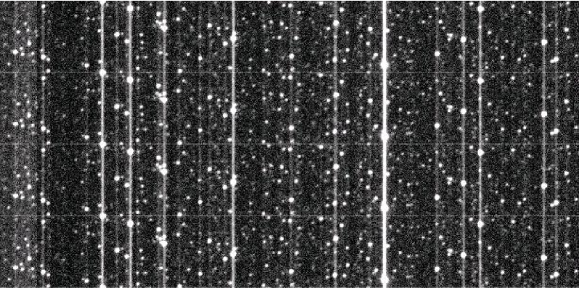
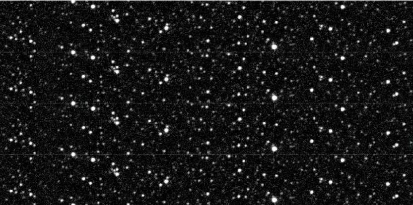
Figure 5: The Background and streak removal was done by subtracting the median value of each column which effectively removed the background and streaks left behind by bright stars.

Figure 6: The histogram of SNR from all lightcurves with more than 10,000 data points.

A complete TAOS data set from 2005 February 7 to 2006 December 31, which amounts to $\sim 4.5\times 10^{9}$ three-telescope measurements was used to search for possible events by objects in Sedna-like orbits. Only measurements from observing runs with more than 10,000 measurements were included in the analysis, because short duration runs could not provide long enough baseline to derive significant statistics. (The duration of a normal data run is 90 minutes, however, occasional interruptions by system failures or bad weather would prevent the system from taking data with the normal duration.) Removing these data runs leaves a total of 199 data runs which amounts to $1.7\times 10^{5}$ star-hours. A plot of the number of star-hours versus SNR for this data set is shown in 6. Furthermore, an additional 26 data runs were found to have significant correlations among the lightcurves for each star (Zhang et al. 2008). Removing these runs leaves us with 173 data runs, corresponding to a total of $1.7\times 10^{5}$ star hours.

Meanwhile, some of the earlier observing runs suffered from guiding problems in the beginning of each run. They all happened near the first 20 seconds when the guider tried to adjust the tracking for the first time. The common feature for this problem is a large displacement in both RA and Dec coordinates of every star. Hence, the first minute of data runs with these large positional offsets were removed.

After all bad lightcurve points were removed, the EW filter was applied to the remaining lightcurves. Any rank triplets beyond our threshold of $F\leq 10^{-8}$ are flagged as candidate events. Most of the candidate events identified by the EW filter turned out to be time coherent. 7 shows two such cases of the number of candidate events within a short period of time (ten seconds). For example, a run with possible high altitude clouds or cirrus would cause overwhelming flux reductions for most stars at the same time. Data runs exhibiting such effects are removed from further analysis. A total of 31 data runs were removed by this cut. On the other hand, during a run with low-lying moving clouds, coherent events would happen only sporadically, when the clouds cover some of the stars in the target field. Data that show such time dependent patterns, which are well characterized and understood, would not be analyzed further for event detection.

As a final selection criterion, we required all candidate events to have at least three consecutive flux measurements below the nominal background level $\langle f\rangle$ used to calculate $W_{i}$. In the end, no candidate occultation events from objects in Sedna-like orbits were found in the first two years of the TAOS data.

Figure 7: Histograms of the number of candidate events vs. time, with ten second binning. A run with possible high altitude clouds or cirrus (left) would cause frequent flux reduction to many stars within a short period of time. Many time coherent events could be observed throughout the entire run. On the other hand, in a run with moving clouds (right), only sporadic coherent events happened at the time when the clouds moved into the our target field.

4 Efficiency Calculation and Event Rate

For a given lightcurve set $l$, the differential occultation event rate $R_{l}$ as a function of diameter $D$ and distance $\Delta$ is

$$\frac{d^{2}R_{l}(D,\Delta)}{dD\,d\Delta}=\frac{d^{2}n(D,\Delta)}{dD\,d\Delta}\frac{v_{\mathrm{rel}}(\phi_{l},\Delta)H_{l}(D,\Delta)}{\Delta^{2}},$$ (7)

where $n(D,\Delta)$ is the number density of objects with diameter $D$ at distance $\Delta$, $v_{\mathrm{rel}}(\phi_{l},\Delta)$ is the relative velocity between occulting object and observer during the data run (see Equation 2), and $H_{l}(D,\Delta)$ is the event width, which is assumed to be the diameter of the first Airy ring of the diffraction profile as discussed in §2. (The subscript on $\phi_{l}$ indicates that the relative velocity depends on the angle between the target star and opposition during the data run, and the subscript on $H_{l}$ indicates that the event cross section depends on the angular size of the target star.)

With the event rate, we can now calculate the number of events expected to be seen for a given star during a given data run, as

$$\frac{d^{2}N_{\mathrm{exp}_{l}}(D,\Delta)}{dD\,d\Delta}=\frac{d^{2}R_{l}(D,\Delta)}{dD\,d\Delta}\,E_{l}\,\varepsilon_{l}(D,\Delta),$$ (8)

where $E_{l}$ is the duration of the data run, and $\varepsilon_{l}(D,\Delta)$ is the efficiency for which occultations by objects of diameter $D$ at distance $\Delta$ are detected in the lightcurve set during the data run.

The efficiency $\varepsilon_{l}(D,\Delta)$ was estimated by a simulation, in which we implanted occultation events in the actual light curves, and processed with the same EW filter. If we added $N_{\mathrm{add}_{l}}(D,\Delta)$ events with diameter $D$ and distance $\Delta$ to a lightcurve set and recover $N_{\mathrm{rec}_{l}}(D,\Delta)$ of them, the detection efficiency is simply $\varepsilon_{l}(D,\Delta)=N_{\mathrm{rec}_{l}}(D,\Delta)/N_{\mathrm{add}_{l}}(D,\Delta)$. Even though the impact parameter and epoch at which an occultation takes place affect if a particular event can be detected, by choosing these parameters randomly over their true distributions, we automatically average the efficiency over these parameters, and they can be ignored. We thus chose the impact parameters uniformly in the interval $[-H_{l}/2,H_{l}/2]$, and the event epoch uniformly in the interval $[t_{0},t_{0}+E_{l}]$, where $t_{0}$ is the start time of the data run.

With $\varepsilon_{l}(D,\Delta)$ known, the total number of events expected to be seen in the entire data set can be estimated from Equation 8. That is,

$$\frac{d^{2}N_{\mathrm{exp}}(D,\Delta)}{dD\,d\Delta}=\sum_{l}\frac{d^{2}R_{l}(D,\Delta)}{dD\,d\Delta}\,E_{l}\,\varepsilon_{l}(D,\Delta),$$ (9)

where the sum is taken over all lightcurve sets in the TAOS data set.

Given the extremely large number of lightcurve sets, we found we could calculate a statistically significant value of the detection efficiency by adding only one simulated event to each lightcurve set. If we add events with diameter $D$ to a fraction $w_{D}$ of all lightcurve sets, and events at distance $\Delta$ to a fraction $w_{\Delta}$ of all lightcurve sets, we can write

$$N_{\mathrm{add}_{l}}(D,\Delta)=w_{D}w_{\Delta}.$$

We thus choose a set of diameters $D$ and a set of corresponding values of $w_{D}$ such that $\sum_{D}w_{D}=1$, and a second set of distances $\Delta$ and corresponding values of $w_{\Delta}$ such that $\sum_{\Delta}w_{\Delta}=1$.

Now there would be only one event in a given lightcurve set, so, taking into account of the weighting factors of $w_{D}$ and $w_{\Delta}$, we have the total number of expected events, expressed in the fully expanded form,

$$\frac{d^{2}N_{\mathrm{exp}}(D,\Delta)}{dD\,d\Delta}=\frac{d^{2}n(D,\Delta)}{dD\,d\Delta}\frac{1}{w_{D}w_{\Delta}}\sum_{l}^{\mathrm{rec}}\frac{v_{\mathrm{rel}}(\phi_{l},\Delta)H_{l}(D,\Delta)E_{l}}{\Delta^{2}},$$ (10)

where the sum is now over all lightcurve sets where an event of diameter $D$ and distance $\Delta$ is recovered. This expression can be simplified as (Zhang et al. 2008),

$$\frac{d^{2}N_{\mathrm{exp}}(D,\Delta)}{dD\,d\Delta}=\frac{d^{2}n(D,\Delta)}{dD\,d\Delta}\,\Omega_{\mathrm{e}}(D,\Delta),$$ (11)

where

$$\Omega_{\mathrm{e}}(D,\Delta)=\frac{1}{w_{D}w_{\Delta}}\sum_{l}^{\mathrm{rec}}\frac{v_{\mathrm{rel}}(\phi_{l},\Delta)H_{l}(D,\Delta)E_{l}}{\Delta^{2}}$$ (12)

is the effective solid angle of the survey.

Equation 11 shows that the number of expected events $N_{\mathrm{exp}}$ in our survey depends on two factors, a model dependent factor $n$ and a survey dependent factor $\Omega_{\mathrm{e}}$. This indicates that the number of events detected in the survey and the value of $\Omega_{\mathrm{e}}$ determined by the efficiency calculation can thus be used to place constraints on $n(D,\Delta)$.

As in Zhang et al. (2008), we used the event simulator described in Nihei et al. (2007) in our efficiency calculation. The distances, diameters, and weighting factors used are shown in Table 1. The weights were chosen to give preference to smaller objects where the detection efficiency is expected to be low in order to improve the statistical accuracy of $\Omega_{\mathrm{e}}$. After implanting simulated events, the exact same selection criteria described above were applied to find which events are recovered. Several example lightcurve sets where simulated events are recovered are shown in 8, and the resulting values of $\Omega_{\mathrm{e}}$ are shown in 9.

Table 1: Distances, diameters, and weighting factors used in efficiency test. The weighting factors are normalized so that $\sum_{D}w_{D}=1$ and $\sum_{\Delta}w_{\Delta}=1$.

$D$ (km)	$w_{D}$	$\Delta$ (AU)	$w_{\Delta}$
0.5	100/785	100	0.2
0.7	100/785	200	0.2
1.0	100/785	300	0.2
1.3	100/785	500	0.2
2.0	100/785	1000	0.2
3.0	100/785
5.0	100/785
10.0	50/785
20.0	30/785
30.0	5/785

Table 2: Distribution of synthetic events in efficiency test

$D$ (km)	100 AU	200 AU	300 AU	500 AU	1000 AU
0.5	0/6409	0/6325	0/6496	0/6361	0/6378
0.7	0/6393	0/6339	0/6392	0/6420	0/6411
1.0	0/6339	0/6363	0/6466	0/6365	0/6453
1.3	0/6260	0/6391	0/6291	0/6357	0/6281
2.0	21/6403	3/6432	0/6382	0/6285	0/6458
3.0	68/6408	23/6366	5/6375	1/6427	0/6296
5.0	207/6302	96/6402	57/6357	21/6398	2/6318
10.0	291/3116	203/3227	172/3285	86/3246	29/3221
20.0	327/1897	291/1927	257/1936	193/2010	96/1855
30.0	78/295	66/311	69/366	51/331	26/310

The ratio of recovered to implanted events for each value of $D$ and $\Delta$ is shown in Table 2. Note that the algorithm did not recover any events with $D<2$ km. Also note that the efficiency for detecting 30 km objects at 100 AU is only about 30%, indicating that a large fraction of the low SNR lightcurve sets used in the analysis are not useful for detecting occultation events at these distances. While including these stars in the analysis lowers the detection efficiency, they have no effect on the resulting values of $\Omega_{\mathrm{e}}$. However, in future analysis runs we will likely set stricter cuts on SNR values to use our computing resources more efficiently.

Figure 8: During the efficiency test, synthetic events were added into TAOS lightcurves. Examples of lightcurves with the synthetic events in three TAOS lightcurves are shown in the upper part of each panel and the corresponding $\eta$ values in the lower part of each panel. Some constants were added to second and third lightcurves to separate them for clarity. The dotted-lines are the $\eta$ value for $F\leq 10^{-8}$. (a) 2 km, 200 AU, $\phi=68.8^{\circ}$ (b) 3 km, 500 AU, $\phi=45.9^{\circ}$, (c) 5 km, 1000 AU, $\phi=34.4^{\circ}$ (d) 10 km, 1000 AU, $\phi=34.4^{\circ}$.

Figure 9: Effective solid angle versus size for different distances from the TAOS efficiency calculation.

Given $\Omega_{\mathrm{e}}$ and the fact that no events were found by the survey, we can set constraints on $n(D,\Delta)$. Because there are no published models of the size and distance distributions of objects in this region, we place constraints on $n(D,\Delta)$ at each value of $\Delta$ listed in Table 1. For the size distribution, we assume a simple power law model of the form

$$\frac{d\,n_{\Delta}(D)}{d\,D}=n_{0}(q-1)\left(\frac{D}{1~{}\mathrm{km}}\right)^{-q},$$ (13)

where $q$ is the slope of the power law, and $n_{0}$ is the number density of objects with $D\geq 1$ km at distance $\Delta$. The expected number of events at distance $\Delta$ is thus

$$N_{\rm exp}(\Delta)=n_{0}\,(q-1)\int^{D_{\mathrm{max}}}_{D_{\mathrm{min}}}\left(\frac{D}{1~{}\mathrm{km}}\right)^{-q}\Omega_{\mathrm{e}}(D,\Delta)\,dD,$$ (14)

where $D_{\mathrm{min}}$, for each distance, is the detection limit of size below which the efficiency goes to zero. We picked $D_{\mathrm{max}}=30$ km because we expected the number density of larger objects to be so small as to provide a negligible contribution to the event rate.

Figure 10: A plot of the the product of the power law size distribution $(D/\rm 1~{}km)^{-q}$ and $\Omega_{\mathrm{e}}(D,\Delta)$ versus diameter $D$ at 100 AU, for several values of $q$. Note that $D^{-q}$ decreases with $D$, and $\Omega_{\mathrm{e}}$ increases with $D$. The product of these two terms is an indicator of the sensitivity of the TAOS system.

The sensitivity of the TAOS system to the size distribution is shown in 10. For $q=3$ the the survey has the maximum sensitivity for objects with $D=3$ km at $\Delta=100$ AU, and the diameter of maximum sensitivity decreases as $q$ is increased. Note that the sensitivity drops off for larger objects, justifying our choice of $D_{\mathrm{max}}=30$ km.

Figure 11: The upper limits of number density with objects larger than 1 km for various q and $\Delta$. Any model with $n_{0}$ above the relevant line is ruled out at the 95% c.l.

We are now ready to bring in observational results to set constraints on the Sedna-like population, including the number density and size distribution. The null detection in the TAOS data means that any model which predicts $N_{\mathrm{exp}}>3$ can be ruled out at the 95% confidence level (c.l.). Resulting upper limits on $n_{0}$ as a function of $q$ are shown in 11. Most of our target fields have ecliptic latitudes $|b|<10^{\circ}$, with more than 93% of the data collected in fields with $|b|<3^{\circ}$, so the upper limits we derived on $n_{0}$ are valid along the ecliptic, assuming that the size distribution is independent of ecliptic longitude.

Figure 12: Upper limit on $n_{\mathrm{s}}$ as a function of $q$ at 100 AU. The diagonal line is the 95% upper limit set by the TAOS survey at 100 AU. The right axis shows the corresponding upper limit on the total expected number of objects larger than Sedna $(N_{\mathrm{s}})$ in the whole sky,assuming an isotropic distribution. Given that one Sedna actually exists, we can also set a lower limit on the surface density. If our assumption of a power-law model is correct, we can exclude size distributions where $N_{\mathrm{s}}<0.05$ (dotted line) at the 95% c.l., which corresponds to a value of $n_{\mathrm{s}}<1.2\times 10^{-6}$ deg^-2.

We know very little about the size distribution of objects in Sedna-like orbits; Sedna is the only object that has been found. Given the assumed power-law size distribution, we calculated the upper limits on the density $n_{\mathrm{s}}$ of objects larger than Sedna by integrating Equation 13,

$$n_{\mathrm{s}}=n_{0}\left(\frac{D_{\mathrm{s}}}{1~{}\mathrm{km}}\right)^{1-q},$$ (15)

where $D_{\mathrm{s}}=1600$ km is the diameter of Sedna. This upper limit on $n_{\mathrm{s}}$ vs. $q$ at 100 AU is shown in 12. Because one Sedna has been found near 100 AU, we can exclude any model that predicts fewer than 0.05 objects with $D\geq D_{\mathrm{s}}$ at the 95% c.l. That is, with the power-law size distribution, any size distribution which yields $n_{\mathrm{s}}<1.21\times 10^{-6}$ deg^-2 is excluded. An interesting consequence is that slopes $q>5.4$ are also excluded. A larger slope means either too few large-sized objects (D=1600 km) to be consistent with the existence of Sedna, or too many small-sized objects ($>$ 1 km) to comply with the null detection by TAOS.

Roques et al. (2006) reported the possible detection of two occultation events consistent with sub-km objects near 200 AU. The resulting 95% c.l. upper and lower limits on $n_{0}$ vs. $q$ are plotted in 13, along with the 95% c.l. upper limit set by TAOS survey at 200 AU. Again, if the assumption of a power law size distribution is valid, the interpretation of these two events as true occultations is consistent with the TAOS upper limit at the 95% c.l. only if $q>7.6$. Note that this result is valid for any population of objects (e.g. Sedna-like objects, the Scattered Disk or Inner Oort Cloud) in this region.

Figure 13: The 95% upper and lower limits on number density were calculated based on two $\sim 600$ m objects found by Roques et al. (2006) and $q$ from 3.0 to 8.0, along with the 95% upper limit set by TAOS survey at 200 AU.

5 Conclusion

We have analyzed the first two years (2005 February to 2006 December) of TAOS data to search for objects in Sedna-like orbits. With the null detection of objects in this region, we are able to set upper limits upon the number density of objects at different distances. Given that one Sedna has been found, we have also placed lower limits on the number density of objects at 100 AU. We also show that the candidate events reported in Roques et al. (2006) are inconsistent with the TAOS data at the 95% c.l. if the size distribution at $\Delta=200$ AU has slope $q<7.6$. We plan to modify the detection algorithm to facilitate an exact calculation of the statistical significance of candidate events, and we will subsequently complete the analysis of the second TAOS data set (January 2007 to December 2008) and report its results in a future paper. We will also expand the analysis to include limits on the populations of Scattered Disk and Inner Oort Cloud objects.

References

- Allen et al. (2001) Allen, R. L., Bernstein, G. M., & Malhotra, R. 2001, in BAAS, Vol. 33, 1404
- Axelrod et al. (1992) Axelrod, T. S., Alcock, C., Cook, K. H., & Park, H.-S. 1992, in ASP Conf. Ser., Vol. 34, Robotic Telescopes in the 1990s, ed. A. V. Filippenko, 171–181
- Bailey (1976) Bailey, M. E. 1976, Nature, 259, 290
- Barucci et al. (2005) Barucci, M. A. et al. 2005, A&A, 439, L1
- Bernstein et al. (2004) Bernstein, G. M. et al. 2004, AJ, 128, 1364
- Bertin & Arnouts (1996) Bertin, E. and Arnouts, S. 1996, A&AS, 117, 393-404
- Born & Wolf (1980) Born, M. & Wolf, E. 1980, Principles of optics (Oxford: Pergamon Press, 1980, 6th corrected ed.)
- Brasser et al. (2007) Brasser, R., Duncan, M. J., & Levison, H. F. 2007, Icarus, 191, 413
- Brown (2008) Brown, M. E. 2008, The Largest Kuiper Belt Objects (The Solar System Beyond Neptune), 335–344
- Brown et al. (2004a) Brown, M. E., Trujillo, C., & Rabinowitz, D. 2004a, ApJ, 617, 645
- Brown et al. (2004b) Brown, M. E. et al. 2004b, in BAAS, Vol. 36, 1068
- Chiang & Brown (1999) Chiang, E. I. & Brown, M. E. 1999, AJ, 118, 1411
- Cook et al. (1995) Cook, K., Alcock, C., Axelrod, T., & Lissauer, J. 1995, in BAAS, Vol. 27, 1124
- Duncan et al. (1987) Duncan, M., Quinn, T., & Tremaine, S. 1987, AJ, 94, 1330
- Emery et al. (2007) Emery, J. P. et al. 2007, A&A, 466, 395
- Fernandez (1980) Fernandez, J. A. 1980, Icarus, 42, 406
- Fernández & Brunini (2000) Fernández, J. A. & Brunini, A. 2000, Icarus, 145, 580
- Gladman & Chan (2006) Gladman, B. & Chan, C. 2006, ApJ, 643, L135
- Ida et al. (2000) Ida, S., Larwood, J., & Burkert, A. 2000, ApJ, 528, 351
- Kenyon & Bromley (2004) Kenyon, S. J. & Bromley, B. C. 2004, Nature, 432, 598
- Kuiper (1974) Kuiper, G. P. 1974, Celestial Mechanics, 9, 321
- Larsen et al. (2007) Larsen, J. A. et al. 2007, AJ, 133, 1247
- Lehner et al. (2009) Lehner, M. J. et al. 2009, PASP, 121, 138
- Monet et al. (2003) Monet, D. G. et al. 2003, AJ, 125, 984
- Morbidelli & Levison (2004) Morbidelli, A. & Levison, H. F. 2004, AJ, 128, 2564
- Nihei et al. (2007) Nihei, T. C. et al. 2007, AJ, 134, 1596
- Oort (1950) Oort, J. H. 1950, Bull. Astron. Inst. Netherlands, 11, 91
- Rice (2007) Rice, J. A. 2007, Mathematical Statistics and Data Analysis, 3rd edn. (Thomson Brooks/Cole)
- Roques et al. (1987) Roques, F., Moncuquet, M., & Sicardy, B. 1987, AJ, 93, 1549
- Roques et al. (2006) Roques, F. et al. 2006, AJ, 132, 819
- Schwamb et al. (2009) Schwamb, M. E., Brown, M. E., & L., R. D. 2009, ApJ, 694, L45
- Stern (2005) Stern, S. A. 2005, AJ, 129, 526
- Weidenschilling (1977) Weidenschilling, S. J. 1977, Ap&SS, 51, 153
- Zhang et al. (2008) Zhang, Z.-W. et al. 2008, ApJ, 685, L157
- Zhang et al. (2009) Zhang, Z.-W. et al. 2009, accepted by PASP