Effects of Spatially Nonuniform Gain on Lasing Modes in Weakly Scattering Random Systems

Abstract

A study on the effects of optical gain nonuniformly distributed in one-dimensional random systems is presented. It is demonstrated numerically that even without gain saturation and mode competition, the spatial nonuniformity of gain can cause dramatic and complicated changes to lasing modes. Lasing modes are decomposed in terms of the quasi modes of the passive system to monitor the changes. As the gain distribution changes gradually from uniform to nonuniform, the amount of mode mixing increases. Furthermore, we investigate new lasing modes created by nonuniform gain distributions. We find that new lasing modes may disappear together with existing lasing modes, thereby causing fluctuations in the local density of lasing states.

I Introduction

Lasing modes in random media behave quite differently depending on the scattering characteristics of the media Cao (2003). In the strongly scattering regime, lasing modes have a nearly one-to-one correspondence with the localized modes of the passive system Vanneste and Sebbah (2001); Jiang and Soukoulis (2002). Due to small mode volume, different localized modes may be selected for lasing through local pumping of the random medium Cao et al. (2000); Vanneste and Sebbah (2001). The nature of lasing modes in weakly scattering open random systems (e.g., Frolov et al. (1999); Ling et al. (2001); Mujumdar et al. (2004)) is still under discussion Wiersma (2008). In systems which are diffusive on average, prelocalized modes may serve as lasing modes Apalkov et al. (2002). In general, however, the quasi modes of weakly scattering systems are very leaky. Hence, they exhibit a large amount of spatial and spectral overlap. For inhomogeneous dielectric systems with uniform gain distributions, even linear contributions from gain induced polarization bring about a coupling between quasi modes of the passive system Deych (2005). Thus, lasing modes may be modified versions of the corresponding quasi modes. However, Vanneste et al. found that when considering uniformly distributed gain, the first lasing mode appears to correspond to a single quasi mode Vanneste et al. (2007). The study was done near the threshold pumping rate and nonlinear effects did not modify the modes significantly. Far above threshold, it was found that lasing modes consist of a collection of constant flux states Türeci et al. (2008). Mode mixing in this regime is largely determined by nonlinear effects from gain saturation.

Remaining near threshold, pumping a local spatial region, and including absorption outside the pumped region found lasing modes to differ significantly from the quasi modes of the passive system Yamilov et al. (2005). This change is attributed to a reduction of the effective system size. More surprisingly, recent experiments Polson and Vardeny (2005); Wu et al. (2006) and numerical studies Wu et al. (2007) showed the spatial characteristics of lasing modes change significantly by local pumping even without absorption in the unpumped region. It is unclear how the lasing modes are changed in this case by local pumping. In this paper, we carry out a detailed study of random lasing modes in a weakly scattering system with a nonuniform spatial distribution of linear gain. Mode competition depends strongly on the gain material properties, e.g., homogeneous vs. inhomogeneous broadening of the gain spectrum. Ignoring gain saturation (usually responsible for mode competition) and absorption, we find that spatial nonuniformity of linear gain alone can cause mode mixing. We decompose lasing modes in terms of quasi modes and find them to be a superposition of quasi modes close in frequency. The more the gain distribution deviates from being uniform, more quasi modes contribute to a lasing mode.

Furthermore, still considering linear gain and no absorption outside the gain region, we find that some modes stop lasing no matter how high the gain is. We investigate how the lasing modes disappear and further investigate the properties of new lasing modes Andreasen and Cao (In press) that appear. The new lasing modes typically exist for specific distributions of gain and disappear as the distribution is further altered. They appear at various frequencies for several different gain distributions.

In Section II, we describe the numerical methods used to study the lasing modes of a one-dimensional (1D) random dielectric structure. The model of gain and a scheme for decomposing the lasing modes in terms of quasi modes is presented. A method to separate traveling wave and standing wave components from the total electric field is introduced. The results of our simulations are presented and discussed in Section III. Our conclusions concerning the effects of nonuniform gain on lasing modes are given in Section IV.

II Numerical Method

The 1D random system considered here is composed of $N$ layers. Dielectric layers with index of refraction $n>1$ alternate with air gaps ($n=1$) resulting in a spatially modulated index of refraction $n(x)$. The system is randomized by specifying different thicknesses for each of the layers as $d_{1,2}=\left<d_{1,2}\right>(1+\eta\zeta)$ where $\left<d_{1}\right>$ and $\left<d_{2}\right>$ are the average thicknesses of the layers, $0<\eta<1$ represents the degree of randomness, and $\zeta$ is a random number in (-1,1).

A numerical method based on the transfer matrix is used to calculate both the quasi modes and the lasing modes in a random structure. Electric fields on the left (right) side of the structure $p_{0}$ ($q_{N}$) and $q_{0}$ ($p_{N}$) travel toward and away from the structure, respectively. Propagation through the structure is calculated via the $2\times 2$ matrix $M$

$$\left(\begin{array}[]{c}p_{N}\\ q_{N}\\ \end{array}\right)=M\left(\begin{array}[]{c}p_{0}\\ q_{0}\\ \end{array}\right).$$ (1)

The boundary conditions for outgoing fields only are $p_{0}=q_{N}=0$, requiring $M_{22}=0$.

For structures without gain, wavevectors must be complex in order to satisfy the boundary conditions. The field inside the structure is represented by $p(x)\exp[in(x)\tilde{k}x]+q(x)\exp[-in(x)\tilde{k}x]$, where $\tilde{k}=k+ik_{i}$ is the complex wavevector and $x$ is the spatial coordinate. For outgoing-only boundary conditions ($M_{22}=0$), $k_{i}<0$. The resulting field distributions associated with the solutions for these boundary conditions are the quasi modes of the passive system.

Linear gain is simulated by appending an imaginary part to the dielectric function $\epsilon(x)=\epsilon_{r}(x)+i\epsilon_{i}(x)$, where $\epsilon_{r}(x)=n^{2}(x)$. This approximation is only valid at or below threshold Jiang et al. (1999). In Appendix A, the complex index of refraction is calculated as $\tilde{n}(x)=\sqrt{\epsilon(x)}=n_{r}(x)+in_{i}$, where $n_{i}<0$. We consider $n_{i}$ to be constant everywhere within the random system. This yields a gain length $l_{g}=1/k_{i}=1/n_{i}k$ ($k=2\pi/\lambda$ is the vacuum wavenumber of a lasing mode) which is the same in the dielectric layers and the air gaps. Note that this gain length is not to be confused with the length of the spatial gain region, which is described below. The real part of the index of refraction is modified by the imaginary part as $n_{r}(x)=\sqrt{n^{2}(x)+n_{i}^{2}}$. A real wavevector $k=2\pi/\lambda$ describes the lasing frequency. The field inside the structure is now represented by $p(x)\exp[i\tilde{n}(x)kx]+q(x)\exp[-i\tilde{n}(x)kx]$. The frequencies and thresholds are located by determining which values of $k$ and $n_{i}$, respectively, satisfy $M_{22}=0$.

Nonuniform gain is introduced through an envelope function $f_{E}(x)$ multiplying $n_{i}$. The envelope considered here is the step function $f_{E}(x)=H(-x+l_{G})$, where $x=0$ is the left edge of the random structure and $x=l_{G}$ is the location of the right edge of the gain region. $l_{G}$ may be chosen as any value between 0 and $L$.

The solutions of the system are given by the points at which the complex transfer matrix element $M_{22}=0$. Where $\operatorname{Re}[M_{22}]=0$ or $\operatorname{Im}[M_{22}]=0$, “zero lines” are formed in the plane of either complex $\tilde{k}$ (passive case) or ($k$, $n_{i}$) (active case). The crossing of a real and imaginary zero line results in $M_{22}=0$ at that location, thus revealing a solution. We visualize these zero lines by plotting $\log_{10}\left|\operatorname{Re}M_{22}\right|$ and $\log_{10}\left|\operatorname{Im}M_{22}\right|$ to enhance the regions near $M_{22}=0$ and using various image processing techniques to enhance the contrast.

The solutions are pinpointed more precisely by using the Secant method. Locations of minima of $|M_{22}|^{2}$ and a random value located closely to these minima locations are used as the first two inputs to the Secant method. Once a solution converges or $|M_{22}|<10^{-12}$, a solution is considered found. This method has proved extremely adept at finding genuine solutions when suitable initial guesses are provided.

Verification of these solutions is provided by the phase of $M_{22}$, calculated as $\theta=\operatorname{atan2}(\operatorname{Im}M_{22},\operatorname{Re}M_{22})$. Locations of vanishing $M_{22}$ give rise to phase singularities since both the real and imaginary parts of $M_{22}$ vanish. The phase change around a path surrounding a singularity in units of $2\pi$ is referred to as topological charge Halperin (1981); Zhang et al. (2007). In the cases studied here, the charge is $+1$ for phase increasing in the clockwise direction and $-1$ for phase increasing in the counterclockwise direction.

Once a solution is found, the complex spatial field distribution may be calculated. Quasi modes $\psi(x)$ are calculated in the passive case and lasing modes $\Psi(x)$ are calculated in the active case. In order to determine whether or not mode mixing occurs (and if so, to what degree) in the case of nonuniform gain, the lasing modes are decomposed in terms of the quasi modes of the passive system. It was found Leung et al. (1997a, b) that any spatial function defined inside an open system of length $L$ [we consider the lasing modes $\Psi(x)$ here] can be expressed as

$$\Psi(x)=\sum_{m}a_{m}\psi_{m}(x),$$ (2)

where $\psi_{m}(x)$ are a set of quasi modes characterized by the complex wavevectors $\tilde{k}_{m}$. The coefficients $a_{m}$ are calculated by

$$a_{m}= i\int_{0}^{L}\left[\Psi(x)\hat{\psi}_{m}(x)+\hat{\Psi}(x)\psi_{m}(x)\right]dx$$

$$+i\left[\Psi(0)\psi_{m}(0)+\Psi(L)\psi_{m}(L)\right],$$ (3)

where

$$\hat{\psi}_{m}(x)=-i\tilde{k}_{m}n^{2}(x)\psi_{m}(x)$$ (4a)

$$\hat{\Psi}(x)=-ik\left[n_{r}(x)+in_{i}f_{E}(x)\right]^{2}\Psi(x).$$ (4b)

The normalization condition is

$$1= i\int_{0}^{L}2\psi(x)\hat{\psi}(x)dx+i\left[\psi^{2}(0)+\psi^{2}(L)\right]$$

$$= i\int_{0}^{L}2\Psi(x)\hat{\Psi}(x)dx+i\left[\Psi^{2}(0)+\Psi^{2}(L)\right].$$ (5)

An advantage of this decomposition method is that a calculation over an infinite system has been reduced to a calculation over a finite system. Error checking is done by using the coefficients found in Eq. (3) to reconstruct the lasing mode intensity distribution with Eq. (2) yielding $R(x)\equiv\sum_{m}a_{m}\psi_{m}(x)$. We define a reconstruction error $E_{R}$ to monitor the accuracy of the decomposition:

$$E_{R}=\frac{\int|\Psi(x)-R(x)|^{2}dx}{\int|\Psi(x)|^{2}dx}.$$ (6)

In general, the field distribution of a mode in a leaky system consists of a traveling wave component and a standing wave component. In Appendix B we introduce a method to separate the two. This method applies to quasi modes as well as lasing modes; we shall consider lasing modes here. At every spatial location $x$, the right-going complex field $\Psi^{(R)}(x)$ and left-going complex field $\Psi^{(L)}(x)$ are compared. The field with the smaller amplitude is used for the standing wave and the remainder for the traveling wave. If $|\Psi^{(R)}(x)|<|\Psi^{(L)}(x)|$ then the standing wave component $\Psi^{(S)}(x)$ and traveling wave component $\Psi^{(T)}(x)$ are

$$\Psi^{(S)}(x)=\Psi^{(R)}(x)+[\Psi^{(R)}(x)]^{*}$$ (7a)

$$\Psi^{(T)}(x)=\Psi^{(L)}(x)-[\Psi^{(R)}(x)]^{*}.$$ (7b)

Further physical insight on lasing mode formation and disappearance, as well as new lasing mode appearance is provided by a mapping of an “effective potential” dictated by the random structure. Local regions of the random medium reflect light at certain frequencies but are transparent to others Kuhl et al. (2008). The response of a structure to a field with frequency $\omega=ck$ can be calculated via a wavelet transformation of the real part of the dielectric function $\epsilon_{r}(x)=n^{2}(x)$ Bliokh et al. (2004). The relationship between the local spatial frequency $q_{res}$ and the optical wavevector $k$ is approximately $q_{res}=2k$ in weakly scattering structures. The Morlet wavelet $\chi$ is expressed as

$$\chi\left(\frac{x^{\prime}-x}{s}\right)=\frac{\pi^{-1/4}}{\sqrt{s}}e^{i\omega_{0}(x^{\prime}-x)/s}e^{-(x^{\prime}-x)^{2}/2s^{2}},$$ (8)

with nondimensional frequency $\omega_{0}$ and Gaussian envelope width $s$ Torrence and Compo (1998). With $\omega_{0}$ fixed, stretching the wavelet through $s$ changes the effective frequency. Wavelets with varying widths are translated along the spatial axis to obtain the transformation

$$W(x,q_{res})=\int\epsilon_{r}(x^{\prime})\chi^{*}\left(\frac{x^{\prime}-x}{s}\right)dx^{\prime}.$$ (9)

where

$$q_{res}=\frac{\omega_{0}+\sqrt{2+\omega_{0}^{2}}}{2s}.$$ (10)

The wavelet power spectrum $|W(x,q_{res})|^{2}$ is interpreted as an effective potential. Regions of high power indicate potential barriers and regions of low power indicate potential wells for light frequency $\omega=q_{res}c/2$.

III Results

A random system of $N=161$ layers is examined in the following as an example of a random 1D weakly scattering system. The indices of refraction of the dielectric layers are $n_{1}=1.05$ and the air gaps $n_{2}=1$. The average thicknesses are $\left<d_{1}\right>=100$ nm and $\left<d_{2}\right>=200$ nm giving a total average length of $\left<L\right>=$ 24100 nm. The grid origin is set at $x=0$ and the length of the random structure $L$ is normalized to $\left<L\right>$. The degree of randomness is set to $\eta=0.9$ and the index of refraction outside the random media is $n_{0}=1$. The localization length $\xi$ is calculated from the dependence of transmission $T$ of an ensemble of random systems of different lengths as $\xi^{-1}=-d\left<\ln T\right>/dL$. The above parameters ensure that the localization length is nearly constant at 200 $\mu$m $\leq\xi\leq 240$ $\mu$m over the wavelength range 500 nm $\leq\lambda\leq$ 750 nm. With $\xi\gg L$, the system is in the ballistic regime.

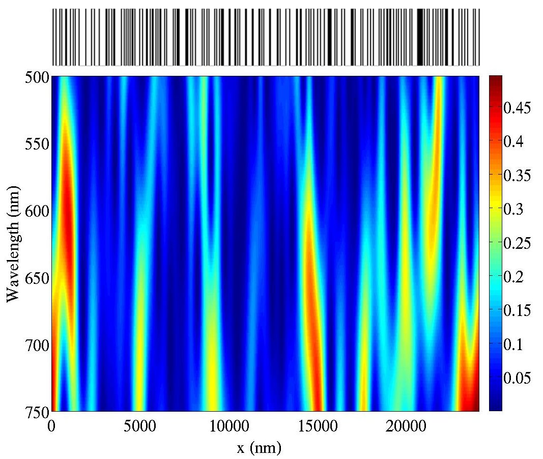
Figure 1: (Color online) Effective potential (wavelet power spectrum) $|W(x)|^{2}$ of the dielectric function $\epsilon_{r}(x)$ as a function of position $x$ and wavelength $\lambda$. Regions of high power indicate potential barriers and regions of low power indicate potential wells where intensities are typically trapped. The black lines on the top represent the spatial distribution of dielectric constant $\epsilon_{r}(x)=n^{2}(x)$.

Figure 1 shows the effective potential of the structure within the wavelength range of interest via a wavelet transformation. We use a nondimensional frequency of $\omega_{0}=6$ Farge (1992) and a spatial sampling step of $\Delta x=2$ nm. The power spectrum $|W(x)|^{2}$ reveals the landscape of the effective potential dictated by the locations and thicknesses of the dielectric layers.

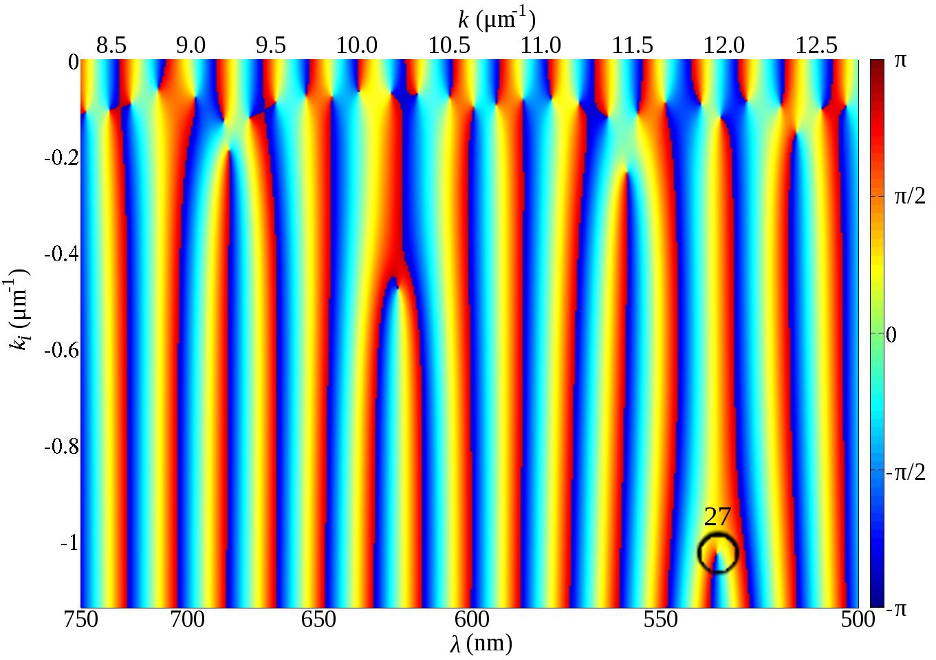
Figure 2: (Color online) A mapping of the phase $\theta$ of $M_{22}$ for the passive 1D random system without gain. The topological charge of all quasi modes seen here is $-1$. Modes are enumerated from left to right. Quasi mode 27 is encircled in black.

Figure 2 is a phase map of $M_{22}$ in the passive case (without gain). The phase singularities mark the quasi modes’ $\tilde{k}$ values and are indicated by phase changes from $-\pi$ to $\pi$ along any lines passing through. The topological charge of all quasi modes is $-1$. Adjacent modes are formed by real and imaginary zero lines of $M_{22}$ that are not connected to one another. We calculated $M_{22}$ for increasingly large $|k_{i}|$ values until machine precision was reached and no additional modes appeared. As previously found Wu et al. (2007), mode frequency spacing is fairly constant in the ballistic regime. The nearly equal spacing of phase singularities in Fig. 2 attests to this.

Figure 3: Normalized intensity $|\psi(x)|^{2}$ of a leaky mode–quasi mode 27 ($\tilde{k}=11.8-i1.03$ $\mu$m^-1) of the passive random 1D structure. The intensity is peaked at the left boundary of the structure, similar to doorway states Okolowicz et al. (2003).

Most quasi modes have similar decay rates except for a few which have much larger decay rates. Modes are enumerated here starting with the lowest frequency mode in our wavelength range of interest. Mode 1 has a wavelength of 748 nm and mode 33 has a wavelength of 502 nm. Most quasi modes have $k_{i}$ values around $-0.1$ $\mu$m^-1. But a few have much larger decay rates, such as mode 27 at $\lambda=532$ nm which has $k_{i}=-1.03$ $\mu$m^-1 (encircled in black in Fig. 2). Figure 3 shows the intensity of mode 27 to be concentrated on one side of the open structure. We observe that it bears similarity to “doorway states” common to open quantum systems Okolowicz et al. (2003). Doorway states are concentrated around the boundary of a system and strongly couple to the continuum of states outside the structure. Therefore, they have much larger decay rates.

For the case of uniform gain, only the lasing modes with large thresholds change significantly from the quasi modes of the passive system. Finding the corresponding quasi modes for lasing modes with large thresholds is challenging due to changes caused by the addition of a large amounts of gain. Thus, we neglect them in the following comparisons. However, there is a clear one-to-one correspondence with quasi modes for the remaining lasing modes. The average percent difference between quasi mode frequencies and lasing mode frequencies is 0.026%. The average percent difference between quasi mode decay rates $k_{i}$ and lasing thresholds (multiplied by $k$ for comparison) $n_{i}k$ is 4.3%. The normalized intensities of the quasi modes $I_{Q}(x)\equiv|\psi(x)|^{2}$ and lasing modes $I_{L}(x)\equiv|\Psi(x)|^{2}$ are also compared. The spatially averaged percent difference between each pair of modes is calculated as $(2/L)\int\left\{|I_{Q}(x)-I_{L}(x)|/[I_{Q}(x)+I_{L}(x)]\right\}dx\times 100$. The averaged difference between intensities of the 3 lasing modes with the largest thresholds (of the large threshold modes not neglected) compared to the quasi modes is 68% while the remaining pairs average a difference of 4.0%.

III.1 Nonuniform Gain Effects on Lasing Mode Frequency, Threshold, and Intensity Distribution

Figure 4 maps the ($k$, $n_{i}$) values of lasing modes as nonuniform gain is introduced by reducing the gain region length from $l_{G}=L$. In this weakly scattering system the intensity distributions of modes are spatially overlapping. This results in a repulsion of mode frequencies Kramer and MacKinnon (1993). As the size of the gain region changes, the envelopes of the intensity distributions change, but for most modes $n_{i}$ is small enough to leave the optical index landscape unchanged. Thus, the modes continue to spatially overlap as the size of the gain region changes and their frequencies remain roughly the same as in the uniform gain case. Similar behavior of lasing mode frequencies can be seen as the gain region length is varied in a simpler cavity with uniform index. Thus, the robustness of frequency is not due to inhomogeneity in the spatial dielectric function. However, the threshold values of the lasing modes change as $l_{G}$ decreases. Due to the limited spatial region of amplification, the thresholds increase. The increase of $n_{i}$ due to the change of threshold, though considerable, is not large enough to significantly impact the lasing frequencies as evidenced by the small change of frequencies as $l_{G}$ decreases.

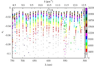
Figure 4: (Color online) Frequencies and thresholds ($k$, $n_{i}$) of the lasing modes of the 1D random structure with gain. Lasing modes 1, 17, 18, and 33 are explicitly marked. The gain region length $l_{G}$ reduces from uniform gain ($l_{G}=L$) to nonuniform gain $l_{G}<L$. The color indicates the value of $l_{G}$ (units of nm) decremented along the layer interfaces. Due to the random thicknesses of the layers, the $l_{G}$ decrements are unequal. Hence, the reason for the unequal spacing of the color code.

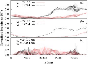
Figure 5: (Color online) Normalized intensity of lasing mode 17 with uniform gain $l_{G}=24100$ nm (red solid lines) and nonuniform gain $l_{G}=14284$ nm (black dashed lines). Gain is only located in the region $0\leq x\leq l_{G}$. (a) Total intensity $|\Psi(x)|^{2}$, (b) traveling wave intensity $|\Psi^{(T)}(x)|^{2}$, and (c) standing wave intensity $|\Psi^{(S)}(x)|^{2}$. Nonuniform gain significantly changes the spatial intensity envelope as well as the standing wave and traveling wave components.

The intensity distributions of the lasing modes also change considerably as $l_{G}$ is reduced. Normalized spatial intensity distributions are given by $|\Psi(x)|^{2}$ after $\Psi(x)$ has been normalized according to Eq. (5). The intensities are sampled with a spatial step of $\Delta x=2$ nm. With uniform gain ($l_{G}=24100$ nm), the intensity of lasing mode 17 ($\lambda=598$ nm) in Fig. 5(a) increases toward the gain boundaries due to weak scattering and strong amplification. When the gain boundary is changed to $l_{G}=14284$ nm, the envelope of the spatial intensity distribution changes dramatically. The intensity increases more rapidly toward the boundaries of the gain region and stays nearly constant outside the gain region but still inside the structure. This change can be understood as $|n_{i}|$ inside the gain region causes the intensity to become larger, while outside the gain region $n_{i}=0$ and the wavevector is real.

To monitor the change in the trapped component of the intensity, $\Psi(x)$ is separated into a traveling wave and a standing wave component via Eq. (7b) (see Appendix B). Figures 5(b) and (c) show the traveling wave and standing wave components of lasing mode 17, respectively. For $l_{G}=L$, the intensity increase toward the structure boundaries is caused mostly by the growth of the traveling wave. The standing wave part is strongest near the center of the system. For $l_{G}=14284$ nm, the standing wave exhibits two peaks, one concentrated near the center of the gain region and the other outside the gain region. However, the standing wave intensity outside the gain region should not be directly compared to the standing wave intensity inside the gain region. The total intensity inside the gain region increases toward the gain boundary in this weakly scattering system. Thus, the amplitude of the field outside the gain region, where there is no amplification, is determined by the total field amplitude at the gain boundary. The randomness of the dielectric function outside the gain region traps part of the wave which results in a relatively large standing wave intensity compared to inside the gain region. However, outside the gain region, there is a net flux toward the right boundary of the system meaning the traveling wave intensity in this region is large as well.

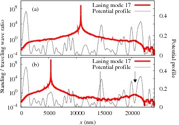
Figure 6: (Color online) Standing/traveling wave ratio $A_{ST}(x)$ (red solid lines) of lasing mode 17 with uniform gain $l_{G}=L$ (a) and nonuniform gain $l_{G}=14284$ nm (b). Gain is located in the regions left of the vertical black solid line. We term the location at which the ratio diverges ($A_{ST}(x)\rightarrow\infty$), the standing wave center (SWC). The potential profile $|W(x)|^{2}$ (black dashed lines) of the dielectric function at the wavelength of mode 17 is overlaid in both (a) and (b).

The relative strength of the standing wave is calculated through the ratio of standing wave amplitude to traveling wave amplitude. The amplitudes are calculated in Appendix B. Depending on whether the prevailing wave is right-going or left-going, the standing/traveling wave ratio is given by

$$A_{ST}(x)=\left\{\begin{array}[]{l}\left|\frac{2\Theta(x)}{\Pi(x)-\Theta(x)}\right|^{2},\Pi(x)>\Theta(x)\\ \left|\frac{2\Pi(x)}{\Theta(x)-\Pi(x)}\right|^{2},\Pi(x)<\Theta(x).\end{array}\right.$$ (11)

Results from considering uniform and nonuniform gain for lasing mode 17 are shown in Fig. 6. Where the standing wave is largest inside the gain region, $|\Psi^{(T)}(x)|=|\Theta(x)-\Pi(x)|=0$ and the ratio $A_{ST}(x)$ is infinite. The location where the ratio is diverging is the position of pure standing wave. Fields are emitted in both directions from this position. The prevailing wave to the right of this standing wave center (SWC) is right-going. The prevailing wave to the left of this SWC is left-going. The SWC of the lasing mode is located near the center of the total system when considering uniform gain in Fig. 6(a). With the size of the gain region reduced in Fig. 6(b), we see that the SWC of the lasing mode (where $A_{ST}(x)\rightarrow\infty$) moves to stay within the gain region. Furthermore, note that this mode has a relatively small threshold (see Fig. 4). We have found that in general, modes with low thresholds have a SWC near the center of the gain region while high threshold modes have a SWC near the edge of the gain region.

The cause for the small peak of $A_{ST}(x)$ outside the gain region can be found in the potential profile of Fig. 1. A slice of the potential profile $|W(x)|^{2}$ at the wavelength of mode 17 ($\lambda=598$ nm) is overlaid on the intensities in Fig. 6. This suggests the standing wave is weakly trapped in a potential well around $x=20500$ nm [marked by an arrow in Fig. 6(b)].

III.2 Mode Mixing

Lasing modes can be expressed as a superposition of quasi modes of the passive system via Eq. (2) for any distribution of gain. Coefficients obtained from the decomposition of the lasing modes in terms of the quasi modes by Eq. (3) offer a clear and quantitative way to monitor changes of lasing modes by nonuniform gain. Using Simpson’s rule for the numerical integrations and a basis consisting of at least 15 quasi modes at both higher and lower frequencies than the lasing mode being decomposed, we consistently find $E_{R}\approx 10^{-4}$.

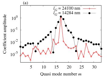
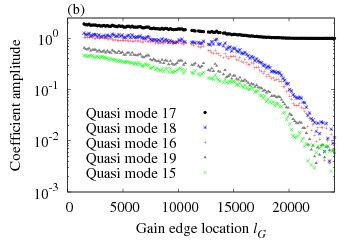
Figure 7: (Color online) Decomposition of lasing mode 17 in terms of passive quasi modes. (a) Decomposition with uniform gain (red crosses) and nonuniform gain (black circles). Leaky quasi modes, i.e., modes with large $|k_{i}|$ such as modes 7, 14, and 23, contribute to lasing modes markedly different than the others. (b) Five largest coefficients from the decomposition of lasing mode 17. As $l_{G}$ is reduced, the amount of mode mixing increases dramatically. The reconstruction error $E_{R}$ for lasing mode 17 is close to $10^{-4}$ until $l_{G}=11000$ nm then rises to $10^{-2}$ at $l_{G}=3200$ nm. Some coefficients are greater than one, which is possible in open systems.

Figure 7(a) shows the decomposition of lasing mode 17 with uniform and nonuniform gain. Beginning with the case of uniform gain ($l_{G}=L$), the largest contribution to lasing mode 17 is from corresponding quasi mode 17. There is a nonzero contribution from other quasi modes on the order $10^{-3}$. This reflects slight differences between the lasing mode profile in the presence of uniform gain and the quasi mode profile Deych (2005); Wu et al. (2007). With the gain region length reduced to $l_{G}=14284$ nm, the coefficients $|a_{m}|^{2}$ from quasi modes closer in frequency to the lasing modes increase significantly; i.e., quasi modes closer in frequency are mixed in. The exceptions are the very leaky quasi modes 7, 14, and 23. Unlike leaky quasi mode 27 shown in Fig. 3, quasi modes 7, 14, and 23 have intensities which are peaked at the right boundary of the structure. It has been observed that when $l_{G}$ reduces and the intensity distribution of lasing mode 17 shifts to the left boundary of the structure, there is less overlap with these leaky quasi modes. Thus, the magnitude of the coefficients associated with the leaky modes reduces as shown in Fig. 7(a).

Figure 7(b) reveals the five largest coefficients $|a_{m}|^{2}$ for lasing mode 17 as $l_{G}$ is incrementally reduced along the dielectric interfaces. While the lasing mode remains dominantly composed of its corresponding quasi mode, neighboring quasi modes mix into the lasing mode significantly. It was shown Deych (2005) that linear contributions from gain induced polarization bring about a coupling between quasi modes of the passive system. This coupling arises solely due to the inhomogeneity of the dielectric function, not the openness of the system. While this interaction may play a role in mode mixing with uniform gain, the effect is small compared to the mode mixing caused by the nonuniformity of the gain. This is clearly demonstrated in Fig. 7(b), where the coefficients from quasi modes close in frequency are orders of magnitude larger for small $l_{G}$ than for $l_{G}=L$.

III.3 Lasing Mode Disappearance and Appearance

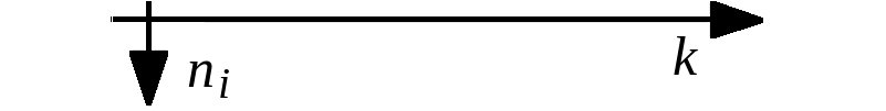
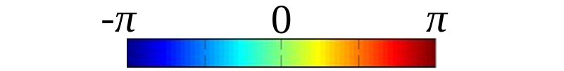
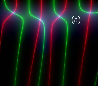
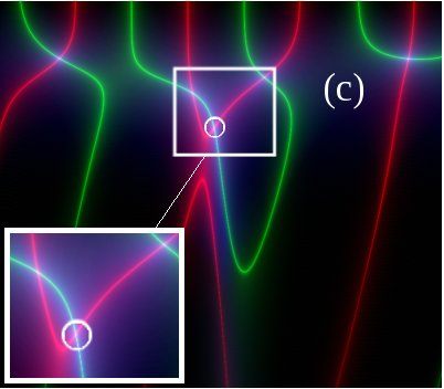
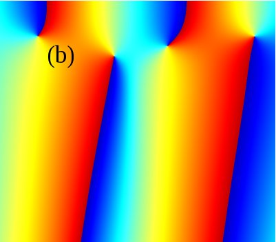
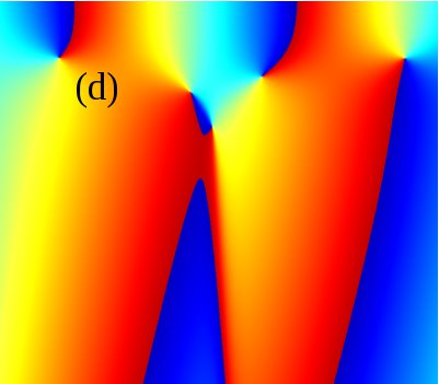
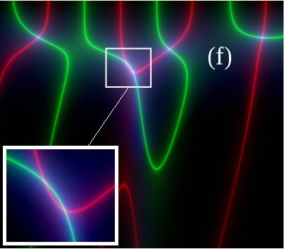
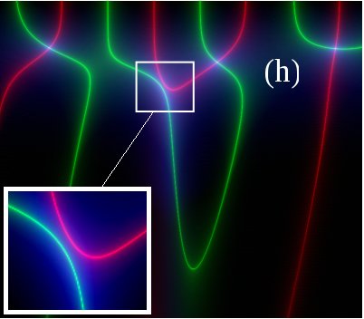
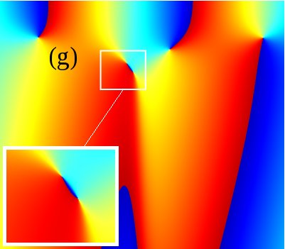
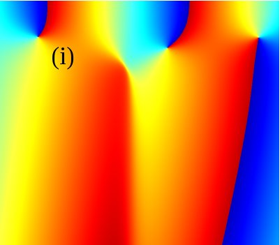
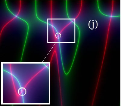
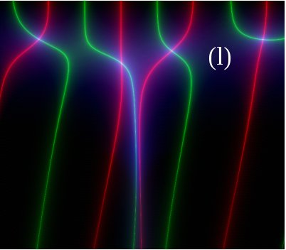
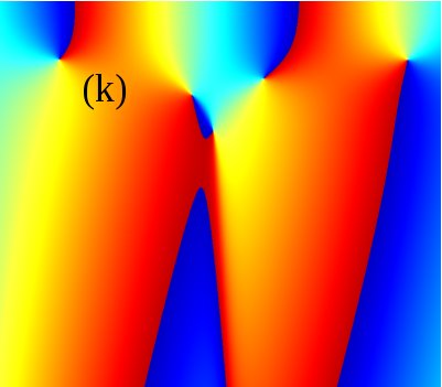
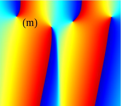
Figure 8: (Color online) (left) Real (green) and Imaginary (red) zero lines of $M_{22}$. Their crossings indicate ($k$, $n_{i}$) values of lasing modes. (right) Phase maps of $M_{22}$. All data are in the ranges ($10.3$ $\mu$m${}^{-1}<k<10.8$ $\mu$m^-1) and ($0\geq n_{i}\geq-0.074$) covering lasing modes 17 and 18 for $l_{G}=14961$ nm (a-b), 14553 nm (c-d), 14523 nm (f-g), 14472 nm (h-i), 14284 nm (j-k), and 14042 nm (l-m). The joining of zero lines in (c) results in the formation of a new lasing mode (new zero line crossing is encircled in white). The inset in (c) is an enlargement of the mode 17 and new mode solutions. In (d), the phase singularity at the new mode has a topological charge of $+1$, opposite to that of mode 17. The real and imaginary zero lines pull apart in (f) so that the mode 17 and new mode solutions are nearly identical. The phase map in (g) reveals the existence of the two phase singularities. The lines completely separate in (h) resulting in the disappearance of mode 17 and the new mode. The phase map in (i) confirms the disappearance of the two modes. This process reverses itself in (j-m) yielding behavioral symmetry around $l_{G}=14472$ nm.

As the size of the gain region reduces we observe that some lasing modes disappear and new lasing modes appear. The existence of new lasing modes in the presence of gain saturation has been confirmed Andreasen and Cao (In press). This phenomenon is not limited to random media, but its occurrence has been observed in a simple 1D cavity with a uniform index of refraction. New lasing modes, to the best of our knowledge, are always created with larger thresholds than the existing lasing modes adjacent in frequency. The disappearance of lasing modes is not caused by mode competition for gain because gain saturation is not included in our model of linear gain. Disappearance/appearance events occur more frequently for smaller values of $l_{G}$. New lasing modes appear at frequencies in between the lasing mode frequencies of the system with uniform gain. These new modes exist only within small ranges of $l_{G}$. We also find that the disappearance events exhibit behavioral symmetry (as explained below) around particular values of $l_{G}$. This disappearance and subsequent reappearance causes a fluctuation of the local density of lasing states as $l_{G}$ changes.

We examine the progression of one representative event in detail. The gaps in the decomposition coefficients for lasing mode 17 in Fig. 7(b), in the range 10500 nm $\leq l_{G}\leq 14500$ nm, indicate lasing mode 17 does not exist for those distributions of gain. Figure 8 shows the real and imaginary zero lines of $M_{22}$ and their accompanying phase maps for $l_{G}=$ 14961 nm, 14553 nm, 14523 nm, 14472 nm, 14284 nm, and 14042 nm. As $l_{G}$ decreases, the zero lines of lasing modes 17 and 18 join as seen in the transition from Fig. 8(a) to (c). This creates a new mode solution (marked by a white circle) with a frequency between lasing modes 17 and 18 and a larger threshold. The existence of a new lasing mode is confirmed by the phase singularity in Fig. 8(d). The new mode is close to mode 17 in the ($k$, $n_{i}$) plane and its phase singularity has the opposite topological charge as seen in Fig. 8(d). As $l_{G}$ decreases further, the joined zero lines forming mode 17 and the new mode pull apart. This causes the two solutions to approach each other in the ($k$, $n_{i}$) plane, i.e., the frequency and threshold of mode 17 increase while the frequency and threshold of the new mode decrease. In Figs. 8(f) and (g), the solutions are so close that they are nearly identical, yet they still represent two separate solutions. Further decreasing $l_{G}$ makes the solutions identical. The zero lines then separate and the phase singularities of opposite charge annihilate each other in Figs. 8(h) and (i). This results in the disappearance of mode 17 and the new mode. The process then reverses itself as $l_{G}$ is decreased further [Figs. 8(j)-(m)] yielding the reappearance of mode 17 and the new mode and their subsequent separation in the ($k$, $n_{i}$) plane. This is the aforementioned behavioral symmetry around $l_{G}=14472$ nm.

Figure 9: (Color online) (a) Standing/traveling wave ratio $A_{ST}(x)$ of the new lasing mode (red) and lasing mode 17 (black) for $l_{G}=14553$ nm (solid lines) and $l_{G}=14523$ nm (dotted lines). The potential profile $|W(x)|^{2}$ (black dashed line) of the dielectric function for this wavelength is overlaid in both (a) and (b) and major potential barriers are marked ➀ through ➃. The ratio $A_{ST}(x)$ of the new lasing mode and lasing mode 17 become more similar an converge on each other as $l_{G}$ reduces. Reducing $l_{G}$ further causes these two lasing modes to first disappear then reappear as the process reverses itself. (b) Standing/traveling wave ratio $A_{ST}(x)$ of the new lasing mode (red) and lasing mode 17 (black) after they have reappeared for $l_{G}=14284$ nm. The ratios are similar to the ratios for $l_{G}=14553$ nm in (a). The vertical black solid line marks the gain edge. The ratios of the modes diverge now as $l_{G}$ is reduced.

Examining the standing/traveling wave ratio of lasing mode 17 and the new lasing mode together with the potential profile $|W(x)|^{2}$ offers some insight of mode annihilation and reappearance in real space. Figure 9 shows the ratio $A_{ST}(x)$ for the new mode and mode 17 along with $|W(x)|^{2}$. The potential profile is very similar for the new mode and mode 17 since their wavelengths are very close. There are four major potential barriers at the mode 17 wavelength ($\lambda=598$ nm) for $x<15000$ nm. This is the spatial region associated with the gain distributions in Fig. 8 where $l_{G}$ is always smaller than 15000 nm. Figure 9 shows them at: $x=$ ➀ 927 nm, ➁ 5200 nm, ➂ 8700 nm, and ➃ 14519 nm. Due to oscillations, the centers of barriers ➁ and ➂ are less well defined. The right edge of the gain region at $l_{G}=14553$ nm is located just to the right of barrier ➃. For $l_{G}=14523$ nm, the right edge of the gain region nears the maximum of barrier ➃. Figure 9(a) shows that for $l_{G}=14553$ nm, the SWC of the new mode is between barrier ➀ and barrier ➁. The SWC of mode 17 is in the middle of the gain region at $x=5300$ nm and its SWC is between barrier ➁ and barrier ➂. Before disappearing, the modes approach each other in the ($k$, $n_{i}$) plane, eventually merge, and their intensity distributions become identical (as evidenced by the trend of their standing/traveling wave ratios). As $l_{G}$ is further reduced and the modes reappear, the behavior of the modes’ ratios $A_{ST}(x)$ (or equivalently, intensity distributions) reverses itself as expected from the behavioral symmetry shown in Fig. 8. At $l_{G}=14284$ nm, the right edge of the gain region has passed barrier ➃ and Fig. 9(b) [with a different horizontal scale than Fig. 9(a)] shows the SWC of the new mode is in roughly the same location as it was for $l_{G}=14553$ nm. The SWC of mode 17 is also in roughly the same location as it was for $l_{G}=14553$ nm.

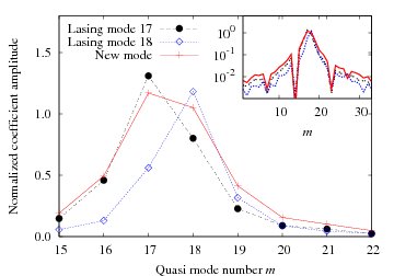
Figure 10: (Color online) Decomposition at $l_{G}=14284$ nm of lasing mode 17 (black circles), lasing mode 18 (blue open diamonds), and the new lasing mode (red crosses) in terms of the quasi modes of the passive system. Lasing modes 17 and 18 are mostly composed of their respective quasi modes while the new mode is dominated by a mixture of both quasi mode 17 and 18. The inset shows the decomposition coefficients of outlying quasi modes for lasing mode 17 (black line), lasing mode 18 (blue line), and the new lasing mode (red line).

The appearance of new lasing modes is unanticipated. In the passive system, the number of standing wave peaks for quasi modes increases incrementally by 1, e.g., quasi mode 17 has 82 peaks and quasi mode 18 has 83 peaks. Lasing modes 17 and 18 behave the same way. How exactly does a new lasing mode fit into this scheme? Though closer in frequency and threshold to lasing mode 17, counting the total number of standing wave peaks of the new lasing mode yields the same number as for lasing mode 18. However, the new lasing mode is somewhat compressed in the gain region having one more peak than lasing mode 18. It is decompressed in the region without gain having one less peak than lasing mode 18.

Comparing the decompositions of the lasing modes in terms of quasi modes helps reveal the character of the new lasing mode. Figure 10 shows the decomposition of the new lasing mode together with the decomposition of lasing modes 17 and 18 at $l_{G}=14284$ nm. The new mode has a slightly larger coefficient amplitude associated with quasi mode 17 than quasi mode 18, but the two amplitudes are nearly equal. We found that as mode 17 and the new mode solutions approach each other by varying $l_{G}$, their coefficient distributions also approach each other until becoming equal as expected from Figs. 8 and 9.

IV Conclusion

We have demonstrated the characteristics of lasing modes to be strongly influenced by nonuniformity in the spatial gain distribution in 1D random structures. While the entire structure plays the dominant role in determining the frequency of the lasing modes, the gain distribution mostly determines the lasing thresholds and spatial distributions of intensity. The gain distribution also appears to be solely responsible for the creation of new lasing modes. We have verified the existence of new lasing modes in numerous random structures as well as dielectric slabs of uniform refractive index. A more thorough investigation of the latter will be described in a future work. All of these changes caused by nonuniform gain take place without the influence of nonlinear interaction between the field and gain medium. Our conclusion is that nonuniformity of the gain distribution alone is responsible for the complicated behavior observed here.

By decomposing the lasing modes in terms of a set of quasi modes of the passive system, we illustrated how the lasing modes change. The contribution of a quasi mode to a lasing mode was seen to depend mostly on its proximity in frequency $k$ and the spatial distribution of gain. The more the gain changed from uniformity, the greater the mixing in of neighboring quasi modes. Thus, great care must be taken even close to the lasing threshold when using the properties of quasi modes to predict characteristics of lasing modes in weakly scattering systems with nonuniform gain or local pumping.

The change of intensity distributions of lasing modes as the size of the gain region is varied appears to be general. With reduction of the size of the gain region, the peak of the standing/traveling wave ratio $A_{ST}(x)$, or the standing wave center (SWC) of the mode, moves to stay within the gain region. Modes with low thresholds have a SWC near the middle of the gain region while high threshold modes have a SWC near the edge of the gain region. Changing the gain distribution thus changes the intensity distributions of lasing modes. The exact modal distributions, however, appear correlated with the potential profile. In the cases studied here, the new lasing mode and lasing mode 17 lay in between two large potential barriers. Decreasing the size of the gain region brought the intensity distributions closer together until they disappeared. These changes took place by varying the edge of the gain region only hundreds of nanometers. Thus, even a slight change in the gain distribution may have drastic consequences for lasing modes.

Appendix A Linear Gain Model

In this appendix, we describe the model used to simulate linear gain in a 1D system. The gain is linear in the sense that it does not depend on the electromagnetic field intensity. The lasing solutions $\Psi(x)$ must satisfy the time-independent wave equation

$$\left[\frac{d^{2}}{dx^{2}}+\epsilon(x,\omega)k^{2}\right]\Psi(x)=0,$$ (12)

with a complex frequency-dependent dielectric function

$$\epsilon(x,\omega)=\epsilon_{r}(x)+\chi_{g}(x,\omega),$$ (13)

where $\epsilon_{r}(x)=n^{2}(x)$ is the dielectric function of the non-resonant background material. The frequency dependence of $\epsilon_{r}(x)$ is negligible. $\chi_{g}(x,\omega)$, corresponding to the susceptibility of the resonant material, is given by

$$\chi_{g}(x,\omega)=\frac{A_{e}N_{A}(x)}{\omega_{a}^{2}-\omega^{2}-i\omega\Delta\omega_{a}},$$ (14)

where $A_{e}$ is a material-dependent constant, $N_{A}(x)$ is the spatially dependent density of atoms, $\omega_{a}$ is the atomic transition frequency, and $\Delta\omega_{a}$ is the spectral linewidth of the atomic resonance. Equation (14) may be simplified by assuming the frequencies of interest $\omega$ are within a few linewidths of the atomic frequency $\omega_{a}$, i.e., $\omega^{2}-\omega_{a}^{2}=(\omega+\omega_{a})(\omega-\omega_{a})\approx 2\omega_{a}(\omega-\omega_{a})$. Equation (14) then reduces to

$$\chi_{g}(x,\omega)\approx\frac{iA_{e}N_{A}(x)}{\omega_{a}\Delta\omega_{a}[1+2i(\omega-\omega_{a})/\Delta\omega_{a}]}.$$ (15)

The frequency-dependent index of refraction is

$$\tilde{n}(x,\omega)= \sqrt{\epsilon(x,\omega)}=\sqrt{\epsilon_{r}(x)+\chi_{g}(x,\omega)}$$

$$= n_{r}(x,\omega)+in_{i}(x,\omega),$$ (16)

which may then be implemented in the transfer matrix method. At this point, let us note that only 2 steps are needed to convert this classical electron oscillator model to real atomic transitions Siegman (1986). First, the radiative decay rate $\gamma_{\parallel}$ may be substituted in to Eq. (15) in place of a few constants. Second, and more importantly, real quantum transitions induce a response proportional to the population difference density $\Delta N_{A}$. Thus, $N_{A}(x)$ should be replaced by $\Delta N_{A}$, the difference in population between the lower and upper energy levels.

Linear gain independent of $\omega$ is obtained by working in the limit $\omega-\omega_{a}\ll\Delta\omega_{a}$, yielding

$$\chi_{g}(x)\approx i\frac{A_{e}\Delta N_{A}(x)}{\omega_{a}\Delta\omega_{a}},$$ (17)

a purely imaginary susceptibility. We can make the definition $\chi_{g}(x)\equiv i\epsilon_{i}(x)$, where $\epsilon_{i}(x)$ is the imaginary part of $\epsilon(x)$. Note that $\epsilon(x)$ may include absorption [$\epsilon_{i}>0$] or gain [$\epsilon_{i}<0$]. We shall only consider gain here. The complex frequency-independent dielectric function now yields a frequency-independent index of refraction $\tilde{n}(x)=n_{r}(x)+in_{i}(x)$ which may be expressed explicitly as

$$n_{r}(x)= \frac{n(x)}{\sqrt{2}}\left[\sqrt{1+\frac{\epsilon_{i}^{2}(x)}{n^{4}(x)}}+1\right]^{1/2}$$

$$n_{i}(x)= \frac{-n(x)}{\sqrt{2}}\left[\sqrt{1+\frac{\epsilon_{i}^{2}(x)}{n^{4}(x)}}-1\right]^{1/2}.$$ (18)

Furthermore, in the main text, we assume $n_{i}$ to be spatially independent. Thus, by solving for $n_{r}(x)$ in terms of $n(x)$ and $n_{i}$, the index of refraction used throughout this paper is given by

$$\tilde{n}(x)= n_{r}(x)+in_{i}$$

$$= \sqrt{n^{2}(x)+n_{i}^{2}}+in_{i}.$$ (19)

Appendix B Standing wave and traveling wave components of the total field

In this appendix, we describe the method that enables one to define a standing wave component and a traveling wave component of the field at each point $x$ of a 1D system.

For an open structure without gain, the field reads

$$\psi(x)=p(x)\exp[in(x)\tilde{k}x]+q(x)\exp[-in(x)\tilde{k}x],$$ (20)

where $\tilde{k}$ is the complex wavevector and $n(x)$ is the index of refraction, the value of which alternates between $n(x)=n_{1}>1$ in dielectric layers and $n(x)=n_{2}=1$ in air gaps. For structures with gain, the field reads

$$\Psi(x)=p(x)\exp[i\tilde{n}(x)kx]+q(x)\exp[-i\tilde{n}(x)kx],$$ (21)

where $\tilde{n}(x)=n(x)+in_{i}$ is the complex index of refraction. We rewrite both equations in the single form

$$E(x)=p(x)\exp[i\tilde{K}(x)x]+q(x)\exp[-i\tilde{K}(x)x],$$ (22)

where $\tilde{K}(x)=K_{r}(x)+iK_{i}(x)$ and $E(x)$ may be either $\psi(x)$ or $\Psi(x)$.

For now, we will consider the field within a single layer in order to simplify the notation. The following results will be valid within any layer. Since within a layer, the coefficients $p(x)$, $q(x)$ and the wavevector $\tilde{K}(x)$ do not depend on $x$, we rewrite Eq. (22) as

$$E(x)=p\exp[i\tilde{K}x]+q\exp[-i\tilde{K}x].$$ (23)

The complex amplitudes $p$ and $q$ of the right-going and left-going fields, respectively, can be written as $p=P\exp[i\varphi]$ and $q=Q\exp[i\phi]$ where $P$ and $Q$ are the real amplitudes which can be chosen positive. The field becomes

$$E(x)= P\exp[-K_{i}x]\exp[i(K_{r}x+\varphi)]$$

$$+Q\exp[K_{i}x]\exp[-i(K_{r}x-\phi)]$$

$$= \Pi(x)\exp[i(K_{r}x+\varphi)]$$

$$+\Theta(x)\exp[-i(K_{r}x-\phi)],$$ (24)

where $\Pi(x)\equiv P\exp[-K_{i}x]$ and $\Theta(x)\equiv Q\exp[K_{i}x]$. Introducing the global phase $\Phi\equiv[\varphi+\phi]/2$ and the difference $\Delta\equiv[\varphi-\phi]/2$, the field reads

$$E(x)= \exp[i\Phi]\{\Pi(x)\exp[i(K_{r}x+\Delta)]$$

$$+\Theta(x)\exp[-i(K_{r}x+\Delta)]\}.$$ (25)

Within a single layer, we can set $\Phi=0$ so that the field becomes

$$E(x)= \Pi(x)\exp[i(K_{r}x+\Delta)]+\Theta(x)\exp[-i(K_{r}x+\Delta)]$$

$$= E^{(R)}(x)+E^{(L)}(x),$$ (26)

where $E^{(R)}(x)$ and $E^{(L)}(x)$ are the right-going and left-going waves, respectively.

We can build a standing wave component with $E^{(R)}(x)$ as

$$E^{(S)}(x)= E^{(R)}(x)+[E^{(R)}(x)]^{*}$$

$$= 2\Pi(x)\cos[K_{r}x+\Delta]$$ (27)

and define the traveling wave component as the remaining part of the total field

$$E^{(T)}(x)= E(x)-E^{(S)}(x)$$

$$= E^{(L)}(x)-[E^{(R)}(x)]^{*}$$

$$= [\Theta(x)-\Pi(x)]\exp[-i(K_{r}x+\Delta)].$$ (28)

Hence, $2\Pi(x)$ and $[\Theta(x)-\Pi(x)]$ are the amplitudes of the standing wave and traveling wave components, respectively. It is also possible to build a standing wave component with $E^{(L)}(x)$ as

$$E^{(S)}(x)= E^{(L)}(x)+[E^{(L)}(x)]^{*}$$

$$= 2\Theta(x)\cos[K_{r}x+\Delta]$$ (29)

so that the traveling wave component reads

$$E^{(T)}(x)= E(x)-E^{(S)}(x)$$

$$= E^{(R)}(x)-[E^{(L)}(x)]^{*}$$

$$= [\Pi(x)-\Theta(x)]\exp[i(K_{r}x+\Delta)].$$ (30)

Comparing both ways of resolving the total field into its two components, we see that in Eq. (28) the traveling wave component is a left-going wave while in Eq. (30) it is a right-going wave. Hence, if in the expression of the field in Eq. (26), the prevailing wave is the right-going wave $\Pi(x)\exp[i(K_{r}x+\varphi)]$ (i.e., $\Pi(x)>\Theta(x)$), we choose the standing and traveling wave components of Eqs. (29) and (30). In the opposite case of $\Pi(x)<\Theta(x)$, we choose the standing and traveling wave components of Eqs. (27) and (28).

Let us note that the imaginary part of the total field $E(x)$ is given in both cases by

$$\operatorname{Im}[E(x)]=[\Pi(x)-\Theta(x)]\sin[K_{r}x+\Delta].$$ (31)

As expected, the presence of a traveling wave component, i.e., $|\Pi(x)-\Theta(x)|\neq 0$, makes $E(x)$ become complex instead of being real for a pure standing wave.

References

- Cao (2003) H. Cao, Waves in Random Media 13, R1 (2003).
- Vanneste and Sebbah (2001) C. Vanneste and P. Sebbah, Phys. Rev. Lett. 87, 183903 (2001).
- Jiang and Soukoulis (2002) X. Jiang and C. M. Soukoulis, Phys. Rev. E 65, 025601 (2002).
- Cao et al. (2000) H. Cao, J. Y. Xu, D. Z. Zhang, S.-H. Chang, S. T. Ho, E. W. Seelig, X. Liu, and R. P. H. Chang, Phys. Rev. Lett. 84, 5584 (2000).
- Frolov et al. (1999) S. V. Frolov, Z. V. Vardeny, K. Yoshino, A. Zakhidov, and R. H. Baughman, Phys. Rev. B 59, R5284 (1999).
- Ling et al. (2001) Y. Ling, H. Cao, A. L. Burin, M. A. Ratner, X. Liu, and R. P. H. Chang, Phys. Rev. A 64, 063808 (2001).
- Mujumdar et al. (2004) S. Mujumdar, M. Ricci, R. Torre, and D. Wiersma, Phys. Rev. Lett. 93, 053903 (2004).
- Wiersma (2008) D. S. Wiersma, Nature Physics 4, 359 (2008).
- Apalkov et al. (2002) V. M. Apalkov, M. E. Raikh, and B. Shapiro, Phys. Rev. Lett. 89, 016802 (2002).
- Deych (2005) L. Deych, Phys. Rev. Lett. 95, 043902 (2005).
- Vanneste et al. (2007) C. Vanneste, P. Sebbah, and H. Cao, Phys. Rev. Lett. 98, 143902 (2007).
- Türeci et al. (2008) H. E. Türeci, L. Ge, S. Rotter, and A. D. Stone, Science 320, 643 (2008).
- Yamilov et al. (2005) A. Yamilov, X. Wu, H. Cao, and A. L. Burin, Opt. Lett. 30, 2430 (2005).
- Polson and Vardeny (2005) R. C. Polson and Z. V. Vardeny, Phys. Rev. B 71, 045205 (2005).
- Wu et al. (2006) X. Wu, A. Yamilov, A. A. Chabanov, A. A. Asatryan, L. C. Botten, and H. Cao, Phys. Rev. A 74, 053812 (2006).
- Wu et al. (2007) X. Wu, J. Andreasen, H. Cao, and A. Yamilov, J. Opt. Soc. Am. B 24, A26 (2007).
- Andreasen and Cao (In press) J. Andreasen and H. Cao, Opt. Lett. (In press).
- Jiang et al. (1999) X. Jiang, Q. Li, and C. M. Soukoulis, Phys. Rev. B 59, R9007 (1999).
- Halperin (1981) B. I. Halperin, in Physics of Defects, edited by R. Balian, M. Kleman, and J. P. Poirier (North-Holland, Amsterdam, 1981).
- Zhang et al. (2007) S. Zhang, B. Hu, Y. Lockerman, P. Sebbah, and A. Z. Genack, J. Opt. Soc. Am. A 24, A33 (2007).
- Leung et al. (1997a) P. T. Leung, S. S. Tong, and K. Young, J. Phys. A 30, 2139 (1997a).
- Leung et al. (1997b) P. T. Leung, S. S. Tong, and K. Young, J. Phys. A 30, 2153 (1997b).
- Kuhl et al. (2008) U. Kuhl, F. M. Izrailev, and A. A. Krokhin, Phys. Rev. Lett. 100, 126402 (2008).
- Bliokh et al. (2004) K. Y. Bliokh, Y. P. Bliokh, and V. D. Freilikher, J. Opt. Soc. Am. B 21, 113 (2004).
- Torrence and Compo (1998) C. Torrence and G. P. Compo, Bull. Amer. Meteorol. Soc. 79, 61 (1998).
- Farge (1992) M. Farge, Annu. Rev. Fluid Mech. 24, 395 (1992).
- Okolowicz et al. (2003) J. Okolowicz, M. Ploszajczak, and I. Rotter, Phys. Rep. 374, 271 (2003).
- Kramer and MacKinnon (1993) B. Kramer and A. MacKinnon, Rep. Prog. Phys. 56, 1469 (1993).
- Siegman (1986) A. E. Siegman, Lasers (University Science Books, Mill Valley, 1986).