RIKEN-TH-173

New Gauged Linear Sigma Models for

8D HyperKähler Manifolds

and

Calabi-Yau Crystals

Yutaka Baba and Ta-Sheng Tai

Theoretical Physics Laboratory, RIKEN, Wako, Saitama 351-0198, JAPAN

We propose two kinds of gauged linear sigma models whose moduli spaces are real eight-dimensional hyperKähler and Calabi-Yau manifolds, respectively. Here, hyperKähler manifolds have $sp(2)$ holonomy in general and are dual to Type IIB $(p,q)$5-brane configurations.

On the other hand, Calabi-Yau fourfolds are toric varieties expressed as quotient spaces. Our model involving fourfolds is different from the usual one which is directly related to a symplectic quotient procedure. Remarkable features in newly-found three-dimensional Chern-Simons-matter theories appear here as well, such as $dynamical$ Fayet-Iliopoulos parameters, one $dualized$ $photon$ and its residual discrete gauge symmetry.

1 Introduction

A gauged linear sigma model (GLSM) in two dimensions [1] is capable of describing a curved geometry (typically a sympletic or Kähler quotient space) through gauge theory language. More precisely, the isometry of the transverse internal space gets partially gauged and chiral multiplets on the worldsheet are coupled to corresponding gauge fields. Then, the curved geometry $\mathbb{C}^{n}//G$ arises as the supersymmetric vacuum (moduli space) of the 2D gauge theory. Note that $G=\mathbb{C}^{\star r}$ stands for $r$ complexified $U(1)$’s with moment maps

$$\mu:~{}\mathbb{C}^{n}\to\mathbb{R}^{r},~{}~{}~{}~{}~{}\mu^{a}=\sum^{n}_{i=1}Q^{a}_{i}~{}|\phi_{i}|^{2},~{}~{}~{}~{}~{}a=1,\dots,r,~{}~{}~{}~{}~{}Q^{a}_{i}:\mathrm{charge~{}assignment}.$$ (1.1)

$\phi_{i}$ parameterizing $\mathbb{C}^{n}$ represents the lowest component of an ${\cal N}$=(2,2) chiral superfield $\Phi_{i}$. Also, $\mu^{a}$’s are called Fayet-Iliopoulos (FI) parameters which bring in $r$ Kähler classes. (1.1) modulo the following gauge symmetry

$$\phi_{i}\sim\phi_{i}~{}e^{i\sum_{a}Q^{a}_{i}\lambda^{a}},~{}~{}~{}~{}~{}~{}\lambda^{a}\in\mathbb{R}$$ (1.2)

is exactly the vacuum manifold denoted as $\mathbb{C}^{n}//G$ or ${\mu}^{-1}(0)/U(1)^{r}$.

Similarly, a hyperKähler quotient space is defined by $\mathbb{H}^{n}///\mathbb{G}$ ($\mathbb{H}^{n}\cong\mathbb{R}^{4n}$) where $\mathbb{G}(\subset{\mathrm{triholomorphic~{}isometry}})$ is generated by vector fields $K$’s with ${\cal L}_{K}g=0$ ($g$: metric) and ${\cal L}_{K}I^{\alpha}=0$. Three complex structures $I^{\alpha}$ $(\alpha=1,2,3)$ are

$$\omega^{\alpha}=d{\cal P}^{\dagger}{\sigma}^{\alpha}\wedge d{\cal P},~{}~{}~{}~{}{\cal P}=(q,\tilde{q}^{\dagger})^{t},~{}~{}~{}~{}{\sigma}^{\alpha}:\mathrm{Pauli~{}matrices}$$ (1.3)

for each $\mathbb{H}$ described by $ds^{2}=|dq|^{2}+|d\tilde{q}|^{2}$ $(q,\tilde{q}\in\mathbb{C})$ and transform as a triplet under $SU(2)$. Our convention is as follows. A quaternion ${\cal Q}=y+{\boldsymbol{y}}~{}(\bar{{\cal Q}}=y-{\boldsymbol{y}})$ with a pure imaginary part ${\boldsymbol{y}}=ui+vj+wk$ $(y,u,v,w\in{\mathbb{R}})$ consists of a pair of complex numbers $(q,\tilde{q})$:

$${\cal Q}=-q+\tilde{q}j,~{}~{}~{}~{}~{}~{}\bar{{\cal Q}}=-q^{\dagger}-j\tilde{q}^{\dagger}.$$ (1.4)

For $n$ quaternions, $r$ moment maps associated with $\mathbb{G}$ under a charge matrix $Q^{a}_{i}$ will read

$$\sum^{n}_{i=1}Q^{a}_{i}~{}{\cal P}_{i}^{\dagger}{\boldsymbol{\sigma}}{\cal P}_{i}={\boldsymbol{\xi}}^{a},~{}~{}~{}~{}~{}~{}{\cal P}_{i}=(q_{i},\tilde{q}^{\dagger}_{i})^{t},~{}~{}~{}~{}~{}~{}a=1,\dots,r$$

or

$$\sum^{n}_{i=1}Q^{a}_{i}\Big{(}|q_{i}|^{2}-|\tilde{q}_{i}|^{2}\Big{)}=\xi^{3a},~{}~{}~{}~{}~{}~{}\sum^{n}_{i=1}Q^{a}_{i}~{}2q_{i}\tilde{q}_{i}=\xi^{1a}-i\xi^{2a}.$$ (1.5)

Here, triplets ${\boldsymbol{\xi}}$’s are given level sets. By definition $\mathbb{H}^{n}///\mathbb{G}$ has real $4(n-r)$ dimensions.

In this note, we propose two kinds of GLSMs which have, respectively, 8D hyperKähler manifolds and Calabi-Yau (CY) 4-folds as their moduli spaces. In the former case, we have followed pioneering works [2, 3, 4]. We extend their ${\cal N}$=(4,4) models to include generic 8D hyperKähler geometries dual to Type IIB $(p,q)$5-brane configurations [6]. Moreover, taking an infra-red (IR) limit leads to frozen kinetic terms of vector-multiplets. By integrating them out, a nonlinear sigma model (NL$\sigma$M) can be realized in the Higgs branch; that is, the quotient space metric is now pulled back onto worldsheet’s kinetic term. The latter case is an ${\cal N}$=(2,2) model which provides instead a CY 4-fold at IR. It is not the traditional one [1] which executes a sympletic quotient because it possesses all key features of 3D ${\cal N}$=2 Chern-Simons-matter theories on a stack of M2-branes probing toric CY 4-folds. Namely, usually F-term conditions (defining a master space) and D-term ones as a whole give a CY 3-fold as the story happens in 4D ${\cal N}$=1 superconformal field theories (SCFT). However, because of the appearance of one $dualized$ $photon$ ${\cal{A}}$ here, the D-term constraint associated with ${\cal{A}}$ becomes redundant due to $dynamical$ Fayet-Iliopoulos (FI) parameters and a 4-fold emerges thereof. Remarkably, we find these properties definitely show up in our model. We demonstrate this mechanism via one explicit example – a 4-fold arising from $\mathbb{C}^{3}/\mathbb{Z}_{3}$.

In section 2, a Taub-NUT (ALF) space constructed by means of hyperKähler quotient and its corresponding GLSM are reviewed. Then, in section 3 we write down our model mentioned above whose Higgs branch probes generic 8D hyperKähler manifolds. Section 4 is devoted to the model probing CY 4-folds. Finally, our results are summarized in section 5.

2 Review: 4D Taub-NUT (ALF) space

To begin with, let us see how a multi-centered Taub-NUT (or ALF) space can be constructed by means of hyperKähler quotient [7, 8]. After then, we go to acquaint ourselves with the GLSM description of it according to [2]. The very quotient procedure is exactly carried out in the Higgs branch of the proposed GLSM at IR. Non-zero hyper-multiplets take their values in a hyperKähler manifold thereof.

As said in section 1, from $\mathbb{H}^{n}\cong\mathbb{R}^{4n}$ one can construct a hyperKähler manifold $\mathbb{H}^{n}///\mathbb{G}$ with $\mathbb{G}$ being triholomorphic, i.e. it does not alter the hyperKähler structure. We will mainly adopt the following triholomorphic right multiplication

$${\cal Q}\to{\cal Q}e^{i\theta},~{}~{}~{}~{}~{}~{}\theta\in(0,4\pi]$$

whose moment map reads

$${\boldsymbol{\mu}}={\cal Q}i\bar{{\cal Q}}=2q\tilde{q}k+\big{(}|q|^{2}-|\tilde{q}|^{2}\big{)}i,~{}~{}~{}~{}~{}~{}(q,\tilde{q})\in\mathbb{C}^{2}.$$ (2.1)

In addition, a right multiplication ${\cal Q}p$ by a unit quaternion $p$ ($p\bar{p}=1$) $\in SU(2)$ does not vary the hyperKähler structure $I^{\alpha}$ of ${\cal Q}$, while a left multiplication $p{\cal Q}$ which keeps the flat metric $ds^{2}=d{\cal Q}d\bar{{\cal Q}}$ invariant but rotates $I^{\alpha}$ plays the role of $SU(2)_{R}$ ($R$-symmetry) under which $(q,\tilde{q}^{\dagger})$ transforms as a doublet. Two operations commute. From now on, we usually do not distinguish between ${\boldsymbol{\mu}}$ being pure imaginary and ${\boldsymbol{r}}=\Big{(}\Re(2q\tilde{q}),-\Im(2q\tilde{q}),|q|^{2}-|\tilde{q}|^{2}\Big{)}\in\mathbb{R}^{3}$ with $|{\boldsymbol{r}}|=|q|^{2}+|\tilde{q}|^{2}$.

Picking up $m+1$ quaternions ${\cal Q}_{a}$ $(a=1,\dots,m+1)$ parameterizing $\mathbb{H}^{m}\times\mathbb{H}\cong\mathbb{R}^{4m}\times\mathbb{R}^{4}$, we want to yield a multi-centered Taub-NUT through dividing $\mathbb{H}^{m+1}$ by the following triholomorphic isometry (${\cal Q}={\cal Q}_{m+1}$):

$${\cal Q}_{a}\to{\cal Q}_{a}e^{it},~{}~{}~{}~{}~{}~{}{\cal Q}\to{\cal Q}+\lambda t,~{}~{}~{}~{}~{}~{}\lambda\in\mathbb{R}.$$

There are $m$ corresponding triplet moment maps:

$${\boldsymbol{m}}_{a}={\cal Q}_{a}i\bar{{\cal Q}}_{a}+\frac{\lambda}{2}({\cal Q}-\bar{{\cal Q}})={\boldsymbol{r}}_{a}+\lambda{\boldsymbol{y}},~{}~{}~{}~{}~{}~{}{\cal Q}=y+{\boldsymbol{y}}.$$ (2.2)

Put into a Taub-NUT form the metric of $\mathbb{H}^{m}\times\mathbb{H}$ ($r_{a}=|{\boldsymbol{r}}_{a}|$):

$$ds^{2}=\sum_{a}d{\cal Q}_{a}d\bar{{\cal Q}}_{a}=\sum_{a}\frac{1}{4}\Big{(}\frac{1}{r_{a}}d{\boldsymbol{r}}_{a}^{2}+{r_{a}}(d\psi_{a}+{\boldsymbol{\omega}}_{a}d{\boldsymbol{r}}_{a})^{2}\Big{)}+dy^{2}+d{\boldsymbol{y}}^{2},$$

$$\nabla\times{\boldsymbol{\omega}}_{a}=\nabla\frac{1}{{r}_{a}},~{}~{}~{}~{}~{}~{}~{}~{}~{}~{}~{}~{}~{}~{}~{}~{}\psi_{a}\in(0,4\pi].$$ (2.3)

By fixing the level set at ${\boldsymbol{m}}_{a}={\boldsymbol{\zeta}}_{a}$ such that ${\boldsymbol{r}}=-\lambda{\boldsymbol{y}}={\boldsymbol{r}}_{a}-{\boldsymbol{\zeta}}_{a}$, it is straightforward to show that (2) becomes

$$ds^{2}=Ud{\boldsymbol{r}}^{2}+\sum_{a}\frac{|{\boldsymbol{r}}+{\boldsymbol{\zeta}}_{a}|}{4}(d\psi_{a}+{\boldsymbol{\omega}}_{a}d{\boldsymbol{r}}_{a})^{2}+dy^{2},$$

$$U_{a}=\frac{1}{4|{\boldsymbol{r}}+{\boldsymbol{\zeta}}_{a}|}+\frac{1}{\lambda^{2}},~{}~{}~{}~{}~{}~{}~{}~{}U=\sum_{a}U_{a}.$$ (2.4)

As a final step, we need to express (2) in terms of ${\boldsymbol{r}}$ and a $gauge$-invariant $\chi$ under moment maps in (2.2), i.e.

$$\chi=\sum_{a}\psi_{a}-\frac{y}{\lambda}.$$

Henceforth, instead of $\psi$’s we use variables like

$$(p_{1},p_{2},\dots,p_{m-1}),~{}~{}~{}~{}~{}~{}~{}~{}~{}~{}p_{\alpha}=\sum_{a=1}^{\alpha}\psi_{a}.$$

The square $\propto(p_{\alpha}+\cdots)^{2}$ is completed and then dropped due to its $gauge$ variance. Finally, we are left with $\chi$ and $y$. Further taking care of the completion of $(y+\cdots)^{2}$, one arrives at

$$ds_{\mathrm{ALF}}^{2}=Ud{\boldsymbol{r}}^{2}+\frac{1}{16}U^{-1}\Big{(}d\chi+(\sum_{a=1}^{m}{\boldsymbol{\omega}}_{a})d{\boldsymbol{r}}\Big{)}^{2}$$

where ${\boldsymbol{\omega}}_{a}$ is evaluated at ${\boldsymbol{r}}+{\boldsymbol{\zeta}}_{a}$.

2.1 Gauged linear sigma model

Take as the prototype the simplest one-nut $TN_{4}$. Let us review its GLSM following Harvey and Jensen [2]. Introduce ${\cal N}$=(4,4) superfield conventions necessary for later convenience:

${\cal N}$=(4,4) vector-multiplet $(\Sigma,\Phi)$
($\Sigma=\frac{1}{\sqrt{2}}\bar{D}_{+}D_{-}V$ is an ${\cal N}$=(2,2) twisted chiral superfield)
${\cal N}$=(4,4) hyper-multiplet $(Q,\tilde{Q})$
${\cal N}$=(4,4) linear hyper-multiplet $(\Psi,P)$

The GLSM Lagrangian ${\cal L}={{\cal L}_{D}}+{{\cal L}_{F}}+{\cal{L}}_{FI}$ for an one-nut $TN_{4}$ consists of

$${{\cal L}_{D}}=\int d^{4}\theta~{}\frac{1}{g^{2}}\Psi^{\dagger}\Psi+\frac{1}{2g^{2}}\Big{(}P^{\dagger}+P+g^{2}\sqrt{2}V\Big{)}^{2}+\frac{1}{e^{2}}\Big{(}-\Sigma^{\dagger}\Sigma+\Phi^{\dagger}\Phi\Big{)}+\Big{(}Q^{\dagger}e^{2V}Q+\tilde{Q}^{\dagger}e^{-2V}\tilde{Q}\Big{)},$$

$${{\cal L}_{F}}=\int d\theta^{+}d\theta^{-}~{}{\cal W}+c.c.,~{}~{}~{}~{}{\cal W}=\Big{(}\sqrt{2}\tilde{Q}\Phi Q-\Psi\Phi\Big{)},$$

$${\cal{L}}_{FI}=\frac{1}{\sqrt{2}}\int d\theta^{+}d\bar{\theta}^{-}~{}t\Sigma+\int d\theta^{+}d\theta^{-}~{}s\Phi+c.c..$$ (2.5)

FI terms are included in ${\cal{L}}_{FI}$ with $(s,t)=(\xi^{1}-i\xi^{2},\xi^{3}+i\theta)$ where superscripts are Cartesian labels. To find out the vacuum, one has to expand (2.1) into (bosonic) component fields. Terms from ${\cal L}_{D}$ in order are listed below (Wess-Zumino gauge of $V$)

$${\text{1st}}:~{}~{}-\frac{1}{2g^{2}}\Big{(}(\partial x^{1})^{2}+(\partial x^{2})^{2}\Big{)}$$

$${\text{2nd}}:~{}~{}-\frac{1}{2g^{2}}\Big{(}2g^{4}(\partial\gamma+A)^{2}+(\partial x^{3})^{2}\Big{)}-g^{2}|\sigma|^{2}$$

$${\text{3rd}}:~{}~{}\frac{1}{e^{2}}(\frac{1}{2}F_{01}^{2}-|\partial\phi|^{2}-|\partial\sigma|^{2})$$

$${\text{4th}}:~{}~{}-|{\cal D}q|^{2}-|{\cal D}\tilde{q}|^{2}-2(|q|^{2}+|\tilde{q}|^{2})|\sigma|^{2}$$ (2.6)

Immediately, a D-term potential (by integrating out $D$ in $V$)

$$V_{D}=-\dfrac{e^{2}}{2}\Big{(}|q|^{2}-|\tilde{q}|^{2}-(x^{3}-\xi^{3})\Big{)}^{2}$$ (2.7)

and F-term potentials (by integrating out $F_{Q}$, $F_{\tilde{Q}}$, $F_{\Phi}$ and $F_{\Psi}$)

$$\begin{cases}V_{\Phi}=-\dfrac{e^{2}}{2}\Big{|}2q\tilde{q}-(x^{1}-ix^{2})+s\Big{|}^{2}\\ V_{Q}+V_{\tilde{Q}}=-2|q|^{2}|\phi|^{2}-2|\tilde{q}|^{2}|\phi|^{2}\\ V_{\Psi}=-g^{2}|\phi|^{2}\end{cases}$$ (2.8)

follow.

Further by taking an infra-red limit ($e^{2}\to\infty$) which decouples the vector-multiplet kinetic term, we find from (2.1) to (2.8) that the $Coulomb$ branch is essentially excluded because of $(\phi,\sigma)\to 0$. We finally obtain the supersymmetric vacuum satisfying

$$|q|^{2}-|\tilde{q}|^{2}=x^{3}-\xi^{3},~{}~{}~{}~{}~{}~{}2q\tilde{q}=x^{1}-ix^{2}-\xi^{1}+i\xi^{2}$$ (2.9)

which is just the standard moment map considered in (2.1). We observe that the massive gauge field $A_{\mu}$ (mass square $g^{2}$) manages to $eat$ (gauge away) one unwanted angular variable variant under (2.9). Given that the metric $|dq|^{2}+|d\tilde{q}|^{2}$ of a quaternion is flat, we express it in a Taub-NUT form with $\varphi\sim\varphi+2\pi$ denoting the triholomorphic $U(1)$ such that

$$|{\cal D}q|^{2}+|{\cal D}\tilde{q}|^{2}\Big{|}_{vacuum}+\frac{1}{2g^{2}}(\partial{\boldsymbol{x}})^{2}+\frac{g^{2}}{2}(\partial\gamma+A)^{2}=$$

$$\Big{(}\frac{1}{2g^{2}}+\frac{1}{4|{\boldsymbol{x}}-{\boldsymbol{\xi}}|}\Big{)}(\partial{\boldsymbol{x}})^{2}+\frac{{|{\boldsymbol{x}}-{\boldsymbol{\xi}}|}}{4}(2A+2\partial\varphi+{\boldsymbol{\omega}}\partial{\boldsymbol{x}})^{2}+\frac{g^{2}}{2}(\partial\gamma+A)^{2},$$

$$\nabla\times{\boldsymbol{\omega}}=-\nabla\frac{1}{|{\boldsymbol{x}}-{\boldsymbol{\xi}}|}.$$ (2.10)

Defining

$$U=\frac{1}{g^{2}}+\frac{1}{2|{\boldsymbol{x}}-{\boldsymbol{\xi}}|},~{}~{}~{}~{}~{}~{}\chi=2(\gamma-\varphi),~{}~{}~{}~{}~{}~{}\partial Y=-\frac{1}{\sqrt{2}}g(\partial\gamma+A),$$

one obtains

$${\cal L}_{IR}=-\Big{(}\frac{1}{2g^{2}}+\frac{1}{4|{\boldsymbol{x}}-{\boldsymbol{\xi}}|}\Big{)}(\partial{\boldsymbol{x}})^{2}-\frac{{|{\boldsymbol{x}}-{\boldsymbol{\xi}}|}}{4}\Big{(}\partial\chi-{\boldsymbol{\omega}}\partial{\boldsymbol{x}}+2\sqrt{2}\frac{\partial Y}{g}\Big{)}^{2}-(\partial Y)^{2}.$$

Further by completing $(\partial Y+\cdots)^{2}$,

$${\cal L}_{IR}=-\frac{1}{2}U(\partial{\boldsymbol{x}})^{2}-\frac{1}{2}U^{-1}\Big{(}\frac{1}{2}\partial\chi-\frac{1}{2}{\boldsymbol{\omega}}\partial{\boldsymbol{x}}\Big{)}^{2}.$$ (2.11)

Note that a remnant $\propto(\partial Y+\cdots)^{2}$ is gauged away by $A_{\mu}$. To conclude, we have found that at IR ($e^{2}\to\infty$) the Higgs branch vacuum manifold manifests itself as a hyperKähler quotient space. Integrating out $A_{\mu}$ then results in a NL$\sigma$M (2.1) with an explicit $TN_{1}$ target metric.

3 8D toric hyperKähler manifold

We are mainly interested in 8D toric hyperKähler manifolds ${\cal M}_{8}={\mathbb{H}}^{n}///\mathbb{G}$ which can be obtained by hyperKähler quotient of quaternions. While ${\cal M}_{8}$=Cone(${{\cal B}}_{7}$) is expressed as a cone, the base seven-manifold ${{\cal B}}_{7}$ is tri-Sasakian and Einsteinian with constant sectional curvature $R_{\mu\nu}=6g_{\mu\nu}$. Recently, this kind of geometry has been studied quite intensively in the context of AdS/CFT because 11D supergravity solutions of the type $AdS_{4}\times{{\cal B}}_{7}$ are dual to various 3D ${\cal N}$=3 SCFTs newly found in [9, 10, 11, 12, 13, 14].

As mentioned before, $\mathbb{G}$ is part of the triholomorphic isometry of ${\mathbb{H}}^{n}$ and preserves its hyperKähler structure. With respect to the remaining triholomorphic $T^{2}$, the metric of ${\cal M}_{8}$ can be put into the following form ($\varphi_{i}\in(0,4\pi]$):

$$\begin{cases}ds^{2}=\frac{1}{2}U_{ij}d{\boldsymbol{x}}_{i}\cdot d{\boldsymbol{x}}_{j}+\frac{1}{2}U^{ij}(d\varphi_{i}+A_{i})(d\varphi_{j}+A_{j})\\ A_{i}=d{\boldsymbol{x}}_{j}\cdot\boldsymbol{\omega}_{ji}=dx^{a}_{j}~{}\omega_{ji}^{a},\quad\partial_{x^{a}_{j}}\omega^{b}_{ki}-\partial_{x^{b}_{k}}\omega_{ji}^{a}=\epsilon^{abc}\partial_{x^{c}_{j}}U_{ki}\end{cases}$$ (3.1)

where $i,j,k=1,2$ and $a,b,c=1,2,3$ (Cartesian label). Conventionally, ${\cal M}_{8}$ is embedded in M-theory and occupies (345678910), i.e. ${\boldsymbol{x}}_{1}=(345)$ and ${\boldsymbol{x}}_{2}=(789)$ while circles $(\varphi_{1},\varphi_{2})$ stands for $(x^{6},x^{10})$. In fact, this metric is so rigid in the sense that it is fully determined once a proper 2 by 2 symmetric matrix $U$ gets specified [6]. Certainly, adding a constant part $U_{\infty}$ to $U$ is still a solution. Issues about $U_{\infty}$ will be addressed below.

In generic non-degenerate cases where the holonomy of ${\cal M}_{8}$ is exactly $sp(2)$ (instead of $sp(1)\times sp(1)$), a fraction $3/16$ out of full 32 SUSY remains and there exist three real covariantly constant spinors rotated by $SO(3)_{R}$ $R$-symmetry of ${\cal M}_{8}$. Since covariantly constant spinors and the triholomorphic isometry commute, the same amount of SUSY survive the duality map which utilizes the above $T^{2}$, say, “$\big{(}$M-theory/two-torus$\big{)}$ $\leftrightarrow$ Type IIB string theory”. Consequently, via the duality chain ${\cal M}_{8}$ gets dual to properly-oriented IIB $(p,q)$5-branes attached on a circle $\tilde{x}^{6}$ (T-dualized $x^{6}$). How a reduced amount of holonomy from $sp(2)$ to $sp(1)\times sp(1)$ which results in totally $1/4$ SUSY occurs? This becomes possible when ${\cal M}_{8}$ just reduces to two orthogonal Taub-NUT spaces occupying $(3456)$ and $(78910)$, respectively (up to some orbifold identification). There may be two kind of situations. One is when $U=U_{\infty}+\Delta U$ happens to factorize into a diagonal form. The other lies in zooming in on the $near$-$horizon$ region (${\boldsymbol{x}}_{1,2}\sim 0$) such that $U_{\infty}$ is gotten rid of and $\Delta U$ may get properly diagonalized.

As advertised, some comments follow from the relation

$$\dfrac{U^{-1}}{\sqrt{\det U^{-1}}}=\dfrac{1}{\Im\tau}\left(\begin{array}[]{cc}|\tau|^{2}&\Re\tau\\ \Re\tau&1\end{array}\right)$$ (3.4)

where we have dropped the subscript $\infty$ for asymptotic $\tau$ and $U$ at infinity. Though (3.4) simply results from translating the asymptotic metric of $T^{2}$ in (3.1) into its complex moduli $\tau$, this correlation does imply an $SL(2,\mathbb{Z})$ covariance of both 5-brane charge vectors and the IIB axio-dilaton $\chi+ie^{-\phi}=\tau_{\infty}$. As a matter of fact, $U_{\infty}$ plays a role of fixing the orientation of 5-branes and subsequently determines the form of $\Delta U$. Therefore as far as preserving six supercharges is concerned, $U_{\infty}$ and $\Delta U$ are not independent. More precisely, the normalization is that when $U_{\infty}={\mathbf{1}}_{2\times 2}$ ($e^{\phi}=g_{s}=1$) a $(1,k)$5-brane is placed relative to a (1,0)5 (NS5) brane occupying (012345) by an angle $\theta=\arctan k$ uniformly on $(3,7)$-, $(4,8)$- and $(5,9)$-plane. In other words, we have measured $\theta$ between two kinds of 5-branes according to [6]

$$\cos\theta=\dfrac{{\boldsymbol{v}}^{\dagger}U^{-1}_{\infty}{\boldsymbol{v}}^{\prime}}{\sqrt{{\boldsymbol{v}}^{2}~{}{\boldsymbol{v}}^{\prime 2}}},~{}~{}~{}~{}~{}~{}~{}~{}~{}{\boldsymbol{v}}=(p,q)^{t}.$$ (3.5)

Combining (3.4) and (3.5), we are able to tell why it is $SL(2,\mathbb{Z})$ rather than $SL(2,\mathbb{R})$ that remains as a symmetry of Type IIB string theory by supersymmetry arguments. Because a correct amount of SUSY should be respected in 11D ${\mathbb{R}}^{1,2}\times{\cal M}_{8}$ due to its hyperKähler nature, dual IIB $(p,q)$5-branes are asked to have specific orientations. That (3.5) is $SL(2,\mathbb{Z})$-invariant leads to $SL(2,\mathbb{Z})$-covariant ${\boldsymbol{v}}$ and $\chi+ie^{-\phi}$ in order to maintain definite 3/16 SUSY necessarily.

3.1 Gauged linear sigma model

Equipped with the above warm-up, we are ready to write down a GLSM which provides triple moment maps from its D- and F-term conditions. It realizes a 8D hyperKähler metric in its Higgs branch thereof at IR upon integrating out auxiliary fields.

To begin with, ${\cal L}={{{\cal L}_{D}}}+{{{\cal L}_{F}}}$ where

$${{{\cal L}_{D}}}=\int d^{4}\theta~{}{\boldsymbol{\Psi}}^{\dagger}{{\cal G}}{\boldsymbol{\Psi}}+\frac{1}{2g_{A}^{2}}(P_{A}^{\dagger}+P_{A}+{g_{A}^{2}}\sqrt{2}{\boldsymbol{p}}\cdot{\boldsymbol{V}})^{2}+\frac{1}{2g_{B}^{2}}(P_{B}^{\dagger}+P_{B}+{g_{B}^{2}}\sqrt{2}{\boldsymbol{q}}\cdot{\boldsymbol{V}})^{2}$$

$$+\sum_{i=1}^{M}\Big{(}\frac{1}{e^{2}_{i}}(-\Sigma_{i}^{\dagger}\Sigma_{i}+\Phi^{\dagger}_{i}\Phi_{i})+H_{i}^{\dagger}e^{2V_{i}}H_{i}+\tilde{H}_{i}^{\dagger}e^{-2V_{i}}\tilde{H}_{i}\Big{)},$$

$${{{\cal L}_{F}}}=\int d\theta^{+}d\theta^{-}~{}{\cal W}+c.c.,~{}~{}~{}~{}~{}~{}{\cal W}=\Big{(}{\boldsymbol{H\tilde{H}}}\cdot{\boldsymbol{\Phi}}\Big{)}-\Big{(}\Psi_{A}{\boldsymbol{p}}+\Psi_{B}{\boldsymbol{q}}\Big{)}\cdot{\boldsymbol{\Phi}}.$$ (3.6)

This is an extension of the original work of Okuyama [3]. Our convention is as follows:

$${\boldsymbol{\Psi}}^{\dagger}=(\Psi_{A},\Psi_{B}),~{}~{}~{}{\cal G}=\left(\begin{array}[]{cc}\dfrac{1}{g_{A}^{2}}&0\\ 0&\dfrac{1}{g_{B}^{2}}\end{array}\right),$$ (3.9)

$$\Psi_{A,B}=\frac{1}{\sqrt{2}}(x_{A,B}^{1}-ix_{A,B}^{2})+\cdots,~{}~{}~{}~{}P_{A,B}=\frac{1}{\sqrt{2}}(-x_{A,B}^{3}+i{g^{2}}\gamma_{A,B})+\cdots,~{}~{}~{}~{}\gamma_{A,B}\sim\gamma_{A,B}+2\pi.$$

Bold symbols (e.g. ${\boldsymbol{p}}$, ${\boldsymbol{q}}$, ${\boldsymbol{\Phi}}$, ${\boldsymbol{V}}$, ${\boldsymbol{H\tilde{H}}}$, etc.) denote $M$-vectors, while $\cdot$ represents the usual vector inner product. Also, ${\cal G}$ will be identified with the $U_{\infty}$ part in (3.1). We have turned off FI parameters which spoil the cone structure of ${\cal M}_{8}$ when one zooms in on the vicinity around the origin. In addition to couplings constants, $({\boldsymbol{p}},{\boldsymbol{q}})$ are the only parameters in (3.1). It becomes transparent later that $({\boldsymbol{p}},{\boldsymbol{q}})$ is responsible for $M$ distinct charge vectors of IIB $(p,q)$5-branes.

We should expand ${\cal L}$ into components fields, integrate out auxiliary $D$ and $F$ fields. Further imposing the infra-red limit $e_{i}^{2}\to\infty$ freezes kinetic terms of vector-multiplets. Henceforth, we are left with (bosonic part only)

$$-\frac{1}{2g_{A}^{2}}(\partial{\boldsymbol{x}}_{A})^{2}-\frac{1}{2g_{B}^{2}}(\partial{\boldsymbol{x}}_{B})^{2}-g_{A}^{2}(\partial\gamma_{A}+{\boldsymbol{p}}\cdot{\boldsymbol{A}})^{2}-g_{B}^{2}(\partial\gamma_{B}+{\boldsymbol{q}}\cdot{\boldsymbol{A}})^{2}$$

$$+\sum_{i}\Big{(}-g_{A}^{2}|p_{i}\sigma_{i}|^{2}-g_{B}^{2}|q_{i}\sigma_{i}|^{2}-|{\cal D}h_{i}|^{2}-|{\cal D}\tilde{h}_{i}|^{2}-2(|h_{i}|^{2}+|\tilde{h}_{i}|^{2})|\sigma_{i}|^{2}\Big{)}$$ (3.10)

and potentials

$$\begin{cases}V_{D}=\sum_{i}-\dfrac{e^{2}_{i}}{2}\Big{(}|h_{i}|^{2}-|\tilde{h}_{i}|^{2}-(p_{i}x_{A}^{3}+q_{i}x_{B}^{3})\Big{)}^{2}\\ V_{F}=\sum_{i}-\dfrac{e^{2}_{i}}{2}\Big{|}2h_{i}\tilde{h}_{i}-p_{i}(x_{A}^{1}-ix_{A}^{2})-q_{i}(x_{B}^{1}-ix_{B}^{2})\Big{|}^{2}-|\phi_{i}|^{2}(2|h_{i}|^{2}+2|\tilde{h}_{i}|^{2}+g_{A}^{2}p_{i}^{2}+g_{B}^{2}q_{i}^{2})\end{cases}$$

A SUSY vacuum accompanied by $(\phi_{i},\sigma_{i})\to 0$ implies $M$ sets of triple moment maps:

$$\begin{cases}|h_{i}|^{2}-|\tilde{h}_{i}|^{2}-(p_{i}x_{A}^{3}+q_{i}x_{B}^{3})=0\\ 2h_{i}\tilde{h}_{i}-p_{i}(x_{A}^{1}-ix_{A}^{2})-q_{i}(x_{B}^{1}-ix_{B}^{2})=0\end{cases}$$ (3.11)

from $V_{D}=V_{F}=0$. It is now clear that the model itself performs a hyperKähler quotient on $M+2$ quaternions by imposing (3.11) which kill $M$ pairs of $(h_{i},\tilde{h}_{i})$.

As before, let us rewrite the flat metric $|dh|^{2}+|d\tilde{h}|^{2}$ of a quaternion into a Taub-NUT form with $\psi$ denoting the triholomorphic $U(1)$, i.e.

$$\sum_{i=1}^{M}|{\cal D}h_{i}|^{2}+|{\cal D}\tilde{h}_{i}|^{2}\Big{|}_{vacuum}$$

$$=\Delta U_{ab}\partial{\boldsymbol{x}}_{a}\cdot\partial{\boldsymbol{x}}_{b}+\sum_{i=1}^{M}\dfrac{|{\boldsymbol{X}_{i}}|}{4}(2A_{i}+2\partial\psi_{i}+{\boldsymbol{\omega}}_{i}\cdot\partial{\boldsymbol{X}}_{i})^{2},~{}~{}~{}~{}a,b=A,B$$

where

$$\Delta U=\sum_{i=1}^{M}\dfrac{1}{4|{\boldsymbol{X}_{i}}|}\left(\begin{array}[]{cc}p_{i}^{2}&p_{i}q_{i}\\ p_{i}q_{i}&q_{i}^{2}\end{array}\right),~{}~{}~{}~{}~{}~{}{\boldsymbol{X}_{i}}=p_{i}{\boldsymbol{x}}_{A}+q_{i}{\boldsymbol{x}}_{B},~{}~{}~{}~{}~{}~{}\nabla\times{\boldsymbol{\omega}}_{i}=-\nabla\frac{1}{|{\boldsymbol{X}_{i}}|}.$$ (3.14)

According to [6], $\Delta U$ corresponds to $M$ dual IIB $(p_{i},q_{i})$5-branes localized at ${\boldsymbol{X}_{i}}=0$ w.r.t. $U_{\infty}={\cal G}$ which can be adjusted to $(\mathrm{const.})\textbf{1}_{2\times 2}$. Since only $\chi_{A}=\gamma_{A}-\sum p_{i}\psi_{i}$ and $\chi_{B}=\gamma_{B}-\sum q_{i}\psi_{i}$ are invariant under the action of moment maps in (3.11), our strategy is to let $M$ massive gauge fields gauge away remaining $gauge$-variant angular variables. To evaluate the term

$$\sum_{i=1}^{M}\dfrac{|{\boldsymbol{X}_{i}}|}{4}(2A_{i}+2\partial\psi_{i}+{\boldsymbol{\omega}}_{i}\cdot\partial{\boldsymbol{X}}_{i})^{2}-\frac{g_{A}^{2}}{2}(\partial\gamma_{A}+{\boldsymbol{p}}\cdot{\boldsymbol{A}})^{2}-\frac{g_{B}^{2}}{2}(\partial\gamma_{B}+{\boldsymbol{q}}\cdot{\boldsymbol{A}})^{2},$$ (3.15)

we adopt variables

$$\tau_{k}=\sum_{i=1}^{k}p_{i}{\cal{B}}_{i},~{}~{}~{}~{}~{}~{}\tilde{\tau}_{k}=\sum_{i=1}^{k}q_{i}{\cal{B}}_{i},~{}~{}~{}~{}~{}~{}{\cal{B}}_{i}=A_{i}+\partial\psi_{i},~{}~{}~{}~{}~{}~{}k=1,\dots,M$$

such that every $2(A_{i}+\partial\psi_{i})$ splits into a sum

$$\frac{\tau_{i}-\tau_{i-1}}{p_{i}}+\frac{\tilde{\tau_{i}}-\tilde{\tau}_{i-1}}{q_{i}}.$$

In dealing with (3.15), we complete in order $(\zeta_{k}\tau_{k}+\eta_{k}\tilde{\tau}_{k}+\cdots)^{2}$ $(\zeta_{k},\eta_{k}=\mathrm{const.})$ from $k=1$ and gauge them away. Finally by substituting the outcome into (3.1) the desired metric form as (3.1) can be reached, i.e.

$${\cal L}_{IR}=-U_{ab}\partial{\boldsymbol{x}}_{a}\cdot\partial{\boldsymbol{x}}_{b}-\frac{1}{4}U^{ab}(\partial\chi_{a}+{\cal E}_{a})(\partial\chi_{b}+{\cal E}_{b}),~{}~{}~{}~{}~{}~{}~{}\chi_{a}\sim\chi_{a}+2\pi,$$

$${{\cal E}}_{a}=-\frac{1}{2}\sum_{i=1}^{M}v_{i,a}{\boldsymbol{\omega}}_{i}\cdot\partial{\boldsymbol{X}}_{i},~{}~{}~{}~{}~{}~{}~{}v_{i}=(p_{i},q_{i}).$$

This is exactly a NL$\sigma$M which pulls back the metric of ${\cal M}_{8}$.

4 ${\cal N}$=(2,2) GLSM for Calabi-Yau fourfold

Let us propose an ${\cal N}$=(2,2) GLSM whose IR moduli space becomes a CY 4-fold. Our superfield conventions are inherited from section 3. The Lagrangian under consideration is ${\cal L}={{{\cal L}_{D}}}+{{{\cal L}_{F}}}$ where

$${{{\cal L}_{D}}}=\int d^{4}\theta~{}\frac{1}{2g^{2}}(P^{\dagger}+P+{\boldsymbol{k}}\cdot g^{2}\sqrt{2}{\boldsymbol{V}})^{2}-\sum_{a=1}^{r}\frac{1}{e^{2}_{a}}\Sigma_{a}^{\dagger}\Sigma_{a}$$

$$+\sum_{i}{\mathcal{H}}_{i}^{\dagger}~{}e^{2V_{h(i)}}{\mathcal{H}}_{i}~{}e^{-2V_{t(i)}}+\sum^{r}_{a=1}\Phi_{a}^{\dagger}e^{2V_{a}}\Phi_{a},$$

$${{{\cal L}_{F}}}=\int d\theta^{+}d\theta^{-}~{}{\cal W}+c.c.,~{}~{}~{}~{}~{}~{}~{}~{}~{}~{}{\boldsymbol{k}}=(k_{1},\cdots,k_{r})\in\mathbb{Z}^{r}.$$ (4.1)

Note that ${\cal W}$ denotes the superpotential and the gauge invariance in the first term of ${\cal L}_{D}$ is maintained by

$${\boldsymbol{k}}\cdot{\boldsymbol{V}}\to{\boldsymbol{k}}\cdot{\boldsymbol{V}}+(\Lambda^{\dagger}+\Lambda),~{}~{}~{}~{}P\to P-\sqrt{2}g^{2}\Lambda,~{}~{}~{}~{}P^{\dagger}\to P^{\dagger}-\sqrt{2}g^{2}\Lambda^{\dagger}.$$

Bi-fundamental chiral fields ${\mathcal{H}}_{i}$ charged under $r$ $U(1)$’s according to a given quiver diagram with $r$ nodes. The subscript $i$ runs over arrows representing bi-fundamental fields in the quiver diagram, while $h(i)$ or $t(i)$ specifies a node on which the head or tail of $i$ ends. In addition, ${\cal W}$ subject to holomorphy is again related to the given quiver. Note that only $P$ of the previous ${\cal N}$=(4,4) multiplet $(\Psi,P)$ enters ${\cal L}$ with the lowest component $x+i\gamma$ ($\gamma\sim\gamma+2\pi$). It is apparent that both ${\cal L}$ and the resultant IR moduli space are characterized only by ${\boldsymbol{k}}$ and the responsible quiver diagram.

First of all, let us expand superfields in ${\cal L}$ into components and integrate out auxiliary $D$ and $F$ fields. Taking $(e_{a}^{2},g^{2})\to\infty$ freezes kinetic terms of fields $(A_{a},\sigma_{a},x)$. What we are left with are (bosonic part only)
1. Kinetic terms of $(h_{i},\phi_{a})$ (bosonic component of $({\mathcal{H}}_{i},\Phi_{a})$
2. A remnant:

$$-g^{2}(\partial\gamma+{\boldsymbol{k}}\cdot{\boldsymbol{A}})^{2}$$ (4.2)

3. A potential:

$$V_{pot}=\sum_{i}|{{h}}_{i}|^{2}|Q^{h(i)}_{i}\sigma_{h(i)}-Q^{t(i)}_{i}\sigma_{t(i)}|^{2}+\sum_{a}2|\sigma_{a}|^{2}|\phi_{a}|^{2}$$

$$+\sum_{a}g^{2}|k_{a}\sigma_{a}|^{2}+\sum_{i}\Big{|}\frac{\partial{\cal W}}{\partial h_{i}}\Big{|}^{2}+\sum_{a}\Big{|}\frac{\partial{\cal W}}{\partial\phi_{a}}\Big{|}^{2}+V_{D},$$

where

$$V_{D}=\sum_{a}\frac{e^{2}_{a}}{2}\Big{(}\sum_{i}(\delta_{h(i)}^{a}Q^{a}_{i}-\delta_{t(i)}^{a}Q^{a}_{i})|h_{i}|^{2}+|\phi_{a}|^{2}-k_{a}x\Big{)}^{2}=\sum_{a}\frac{e^{2}_{a}}{2}D_{a}^{2}$$ (4.3)

The vacuum manifold ${\cal M}$ is determined by

$$\sigma_{a}=\phi_{a}=0~{}~{}~{}~{}~{}~{}D_{a}=0,~{}~{}~{}~{}~{}~{}{d{\cal W}}=0.$$ (4.4)

Several comments follow. A distinguishing feature departing from those dealt with in previous sections is that by means of $\gamma$’s e.o.m. one gauge field ${\cal A}={\boldsymbol{k}}\cdot{\boldsymbol{A}}$ in (4.2) can be dualized into a scalar $-\gamma$. In the context of 3D Yang-Mills-Chern-Simons theory, ${\cal A}$ is referred to as a $dual$ $photon$. Together with $V_{D}=0$ we can understand that the model itself executes rather a $sympletic$ quotient over complex variables $h_{i}$ than a hyperKähler one.

Let us analyze the moduli space in detail from both field-theoretical and geometrical grounds.
1. The constraint $\sum_{a}D_{a}=0$ in (4.3) characterizes the decoupled diagonal $U(1)$ and implies as well that $\sum_{a}k_{a}=0$ or the vector ${\boldsymbol{k}}$ is orthogonal to $(1,\cdots,1)$. To this end, one has only $(r-2)$ linearly independent D-term conditions [17]:

$$\sum_{a}\ell_{a}D_{a}=0,~{}~{}~{}~{}~{}~{}~{}~{}~{}~{}~{}~{}{\boldsymbol{\ell}}\in\mathrm{Ker}({\boldsymbol{k}}),~{}~{}~{}~{}~{}~{}~{}~{}~{}~{}~{}~{}{\boldsymbol{\ell}}\neq(1,\cdots,1).$$

This fact is consistent with that we have a dualized $\cal{A}$ and leads naturally to ${\cal M}=\{d{\cal W}=0\}//C^{\star r-2}$ which is a CY 4-fold by definition emerging from a 3-fold. Namely, ${\cal M}=\{d{\cal W}=0\}//C^{\star r-1}$ is a CY 3-fold because its derivation is just the same with that of 4D ${\cal N}$=1 SCFTs on a bunch of D3-branes probing CY₃ cones.

2. Geometrically, an ungauged $U(1)$ ${\cal{A}}$ suggests the existence of an $S^{1}$ in the vacuum moduli space correspondingly. According to $V_{D}=0$, we can thus describe ${\cal M}$ as a 3-fold fibered on a real line $x$ with a circle bundle fibered over them with non-trivial first Chern class [18, 19]. We find that the field $x$ in (4.3) (or $V_{D}=0$) serves as $dynamical$ FI parameters and plays the very role of giving varying Kähler classes for the fibered 3-fold.

3. Let us elaborate on arguments about the $surviving$ $S^{1}$ bundle associated with ${\cal{A}}$. For conceptual convenience, we can first think of it as $\gamma$ charged logarithmically under $r$ $U(1)$’s:

$$\gamma\to\gamma+\sum_{a=1}^{r}k_{a}\lambda_{a},~{}~{}~{}~{}~{}~{}~{}~{}\gamma\sim\gamma+2\pi.$$ (4.5)

Consequently, (4.5) defines a one-parameter gauge transformation ${\boldsymbol{\lambda}}=t(k_{1},\cdots,k_{r})$. We find that $\gamma$ is especially helpful when one wants to determine the correct periodicity of $S^{1}$. In fact, there may remain some discrete amount of gauge symmetry $\Gamma$ of $\cal{A}$ such that $\Gamma$ shrinks the circumference of $S^{1}$ to $2\pi/gcd({\boldsymbol{k}})$. This is apparent from the expression of ${\boldsymbol{\lambda}}$. Let us put things in an inverse way. From (4.2) $\cal{A}$ is spontaneously broken once $\gamma$ acquires a vev $\gamma_{0}$. But if there exists $f=gcd({\boldsymbol{k}})$ with $\gamma_{0}=f\gamma^{\prime}_{0}+{2m\pi}$ $(m\in\mathbb{Z})$, the gauge fixing becomes incomplete due to a factor ${2m\pi}/{f}$. This soon means that the gauge symmetry of $\cal{A}$ is only spontaneously broken down to a discrete extent. To conclude, we should at the end divide ${\cal M}$ further by $\Gamma$. All these are directly reminiscent of the novel mechanism in newly-developed 3D ${\cal N}$=2 Chern-Simons-matter theories [20]. Therefore, it turns out that, up to a discrete quotient $\Gamma$, ${\cal M}=\{d{\cal W}=0\}//C^{\star r-2}$ where additional real two dimensions result effectively from degrees of freedom of $x+i\gamma\subset P$.

4.1 Toric geometry

Let us review quickly stuffs about toric varieties which are highly helpful when one lifts a toric CY₃ to a toric CY₄. In general, a toric variety $V$ is expressed as $\mathbb{C}^{n}\backslash F//\mathbb{C}^{\star{\cal G}}$ and can be summarized pictorially by a toric diagram consisting of $n$ $d$-vectors $\nu_{i}\in\mathbb{Z}^{d}$ $(d=n-{\cal G})$ subject to

$$\sum_{i=1}^{n}~{}Q^{A}_{i}~{}\nu_{i}=0,~{}~{}~{}~{}~{}~{}A=1,\dots,{\cal G},~{}~{}~{}~{}~{}~{}Q^{A}_{i}:\mathrm{charge~{}matrix}.$$ (4.6)

By imposing the Calabi-Yau condition: $\sum_{i}Q^{A}_{i}=0$  $\forall A$, these $\nu$’s can be written as $\nu_{i}=(1,\cdots)^{t}$ and are called toric data of a toric CY $d$-fold. For $d$=3, toric data are plotted on a plane, while $d$=4 toric data are encoded in 3D lattice points which define a convex polytope – $crystal$. This is why we adopt the name $crystal$ in our title page because CY 4-folds are under consideration.

Let us talk about the geometric meaning of toric data. Every $\nu_{i}$ assigns a shrinking 1-cycle out of $T^{d}$ at the $i$-th facet of the boundary $\partial{\cal{C}}_{+}$ where ${\cal{C}}_{+}$ denotes a cone in $\mathbb{Z}^{d}$ over which $T^{d}$ is fibered over. In $d$=3 cases, lines where two facets meet will altogether constitute a $web$ diagram which in turn represents a tree formed by multiple semi-infinite NS5-branes. Although we will not go further to details, interested readers are encouraged to consult [16].

4.2 Calabi-Yau crystal

Though lifting 3-folds to 4-folds has been studied quite heavily to date, let us just pick up one canonical example $\mathbb{C}^{3}/\mathbb{Z}_{3}$ discussed also in [17, 24, 19]. Here, $\mathbb{Z}_{3}$ is embedded in the Hopf $U(1)$ bundle of $\mathbb{C}^{3}$ whose action is

$$(z_{1},z_{2},z_{3})\to(\epsilon z_{1},\epsilon z_{2},\epsilon z_{3}),~{}~{}~{}~{}~{}~{}~{}~{}~{}\epsilon=e^{2\pi i/3}.$$ (4.7)

4.2.1 $\mathbb{C}^{3}/\mathbb{Z}_{3}$

A stack of D3-branes probing $\mathbb{C}^{3}/\mathbb{Z}_{3}$ [25, 26] has nine bi-fundamental chiral superfields on its worldvolume gauge theory with a superpotential (though we will focus on its abelian version)

$${\cal W}\propto\epsilon^{IJK}\mathop{\rm Tr}(X_{I}Y_{J}Z_{k}),~{}~{}~{}~{}~{}~{}~{}~{}~{}I,J,K=1,2,3.$$ (4.8)

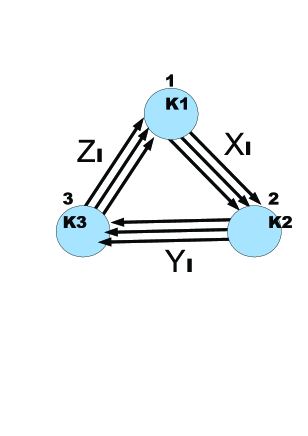
Figure 1: A quiver diagram for $\mathbb{C}^{3}/\mathbb{Z}_{3}$. Three nodes are labeled by integers $(k_{1},k_{2},k_{3})$. Three sets of chiral superfields are denoted as $(X_{I},Y_{I},Z_{I})$ $(I=1,2,3)$.

In Figure 1, three nodes denote three gauge groups and hence $(3-1)$ D-term conditions. In addition, $d{\cal W}=0$ renders four more constraints

$$X_{1}Y_{2}=X_{2}Y_{1},~{}~{}~{}~{}~{}~{}X_{2}Y_{3}=X_{3}Y_{2},~{}~{}~{}~{}~{}~{}(X,Y)\leftrightarrow(Y,Z).$$ (4.9)

Instead, we can $solve$ (4.9) via $X_{I}=u_{1}v_{I}$, $Y_{I}=u_{2}v_{I}$ and $Z_{I}=u_{3}v_{I}$ $(I=1,2,3)$ accompanied by a D-term like condition:

$$|u_{1}|^{2}+|u_{2}|^{2}+|u_{3}|^{2}-|v_{1}|^{2}-|v_{2}|^{2}-|v_{3}|^{2}=0.$$ (4.10)

${\cal M}_{F}=\{d{\cal W}=0\}$ can then be thought of as $\mathbb{C}^{6}//\mathbb{C}^{\star}_{(1,1,1,-1,-1,-1)}$. Alternatively, the following exact sequence

$$0\to\mathbb{Z}\stackrel{{\scriptstyle Q^{t}}}{{\to}}\mathbb{Z}^{6}\stackrel{{\scriptstyle T}}{{\to}}\mathbb{N}\to 0$$ (4.11)

reveals the same thing. It merely says mathematically ${\cal M}_{F}$ can be regarded as $\mathbb{C}^{6}//\mathbb{C}^{\star}$ where the action of $\mathbb{C}^{\star}$ is spelt out by $Q$. More precisely, one can express ${\cal M}_{F}$ as a cone $\mathbb{M}_{+}$ in $\mathbb{M}=\mathbb{Z}^{6}$. Its dual cone (toric data) $\mathbb{N}_{+}$ in $\mathbb{N}=\mathrm{Hom}(\mathbb{M},\mathbb{Z})$ is generated by six lattice points, i.e. $T$: $\mathbb{Z}^{6}\to\mathbb{N}$. By definition Ker($T$) is the image of $Q^{t}$, so the cokernel of $Q^{t}$ is isomorphic to $T$ ($Q$: 1 by 6 matrix). To get a 3-fold, we need to incorporate D-term constraints as well. In summary, we can obey three steps below [26]:
1. Introduce $U$ (5 by 6 matrix) with $UT^{t}=1$ and $V$ (2 by 5 matrix). $V$ encodes two D-term constraints on five independent variables as indicated in (4.9)
2. Concatenate $VU$ (2 by 6 matrix) and $Q$ to yield $Q^{\prime}$ (3 by 6 matrix)
3. Computing the cokernel of $Q^{\prime t}$ gives us desired toric data in terms of a map ${\cal{T}}$: $\mathbb{Z}^{6}\to\mathbb{Z}^{3}$

To have a 4-fold we need to use a new $V$ involving only one linearly-combined D-term constraint (irrelevant to ${\cal{A}}$) out of three nodes and repeat the above procedure. Instead of this approach, a more convenient one figured out in [17] is to directly perform one more quotient on previous $(u_{I},v_{I})$ by another $\mathbb{C}^{\star}$: $(k_{1}+k_{2},-k_{1},-k_{2},0,0,0)$. Translating this into the action on $(X_{I},Y_{I})$, one easily realizes that it is the combination $-k_{2}Q_{1}+k_{1}Q_{2}$ orthogonal to ${\boldsymbol{k}}\cdot{\boldsymbol{Q}}$ with ${\boldsymbol{k}}=(k_{1},k_{2},k_{3}=-k_{1}-k_{2})$. See Table 1 for informations about $Q_{i}$ responsible for the $i$-th node.

Table 1: Nine bi-fundamental chiral matters charged under three gauge groups in the case of ${\mathbb{C}}^{3}/{\mathbb{Z}}_{3}$

	$X_{1}$	$X_{2}$	$X_{3}$	$Y_{1}$	$Y_{2}$	$Y_{3}$	$Z_{1}$	$Z_{2}$	$Z_{3}$
$Q_{1}$	-1	-1	-1	0	0	0	1	1	1
$Q_{2}$	1	1	1	-1	-1	-1	0	0	0
$Q_{3}$	0	0	0	1	1	1	-1	-1	-1

Arbitrary ${\boldsymbol{k}}$ encountered in (4) meet the requirement $\sum_{a}k_{a}=0$. Also, we may demand $gcd(k_{1},k_{2})=1$ technically in order to avoid a further discrete quotient $\Gamma$ explained around (4.5).

All in all, via $(k_{1},k_{2},)=(2p-k,k-p)$ we end up with an eight cone over a seven Sasaki-Einstein base denoted as $Y^{p,k}({\mathbb{CP}}^{2})$. Its toric data are [17]:

$$w_{1}=(0,0,0),~{}~{}w_{2}=(0,0,p),~{}~{}w_{3}=(1,0,0),$$

$$w_{4}=(0,1,0),~{}~{}w_{5}=(-1,-1,k),~{}~{}w_{0}=(0,0,k-p).$$ (4.12)

These six vectors do form a 3D crystal as was shown in [27] with an additional vector $w_{0}$ standing for a resolution, provided $p\leq k\leq 2p$. See [17] for more details.

5 Summary

In this short note we have studied two kinds of GLSMs whose vacuum moduli spaces are real eight-dimensional hyperKähler and Calabi-Yau manifolds, respectively.

The Higgs branch of the former ${\cal N}$=(4,4) GLSM manifests itself as a generic 8D hyperKähler quotient space at the infra-red regime. On the other hand, the latter ${\cal N}$=(2,2) GLSM has a more flexible superpotential ${\cal W}$ as well as chiral matter contents spelt out by a quiver diagram. Usually, D- and F-term constraints give rise to a toric CY 3-fold just as in familiar 4D ${\cal N}$=1 SCFT setups. Nevertheless, owing to a novel mechanism introduced in section 4, 3-folds are promoted to 4-folds exactly the same way as what happens in recently-developed 3D ${\cal N}$=2 Chern-Simons-matter theories which have toric CY 4-folds as their moduli spaces. In words, in addition to the diagonal gauge field $\sum_{a}A_{a}$, an ungauged dual photon ${\cal{A}}=\sum_{a}k_{a}A_{a}$ as well does not enter the quotient process due to $dynamical$ Fayet-Iliopoulos parameters. Therefore, the moduli space dimension is enhanced from six to eight. The extra two dimensions effectively result from degrees of freedom of a chiral superfield $P$. Parameters $k_{a}$ in our 2D Lagrangian satisfying $\sum_{a}k_{a}=0$ are arbitrary integers. Their role is analogous to 3D quiver Chern-Simons levels. We discussed the whole story via a very well-developed 3-fold $\mathbb{C}^{3}/\mathbb{Z}_{3}$.

References

[1]
E. Witten,
Nucl. Phys. B 403, 159 (1993)
[arXiv:hep-th/9301042].
[2]
J. A. Harvey and S. Jensen,
JHEP 0510 (2005) 028
[arXiv:hep-th/0507204].
[3]
K. Okuyama,
JHEP 0508 (2005) 089
[arXiv:hep-th/0508097].
[4]
K. Okuyama,
Phys. Lett. B 668 (2008) 153
[arXiv:0807.0047 [hep-th]].
[5]
D. Forcella, A. Hanany, Y. H. He and A. Zaffaroni,
JHEP 0808 (2008) 012
[arXiv:0801.1585 [hep-th]].
[6]
J. P. Gauntlett, G. W. Gibbons, G. Papadopoulos and P. K. Townsend,
Nucl. Phys. B 500 (1997) 133
[arXiv:hep-th/9702202].
[7]
G. W. Gibbons and P. Rychenkova,
Commun. Math. Phys. 186 (1997) 585
[arXiv:hep-th/9608085].
[8]
E. Witten,
JHEP 0906 (2009) 067
[arXiv:0902.0948 [hep-th]].
[9]
Y. Imamura and K. Kimura,
Prog. Theor. Phys. 120 (2008) 509
[arXiv:0806.3727 [hep-th]].
[10]
D. L. Jafferis and A. Tomasiello,
JHEP 0810 (2008) 101
[arXiv:0808.0864 [hep-th]].
[11]
S. Hohenegger and I. Kirsch,
JHEP 0904 (2009) 129
[arXiv:0903.1730 [hep-th]].
[12]
D. Gaiotto and D. L. Jafferis,
“Notes on adding D6 branes wrapping in ,”
arXiv:0903.2175 [hep-th].
[13]
Y. Hikida, W. Li and T. Takayanagi,
JHEP 0907 (2009) 065
[arXiv:0903.2194 [hep-th]].
[14]
M. Fujita and T. S. Tai,
JHEP 0909 (2009) 062
[arXiv:0906.0253 [hep-th]].