Tropical Nevanlinna theory and second main theorem

1. Introduction

Tropical Nevanlinna theory, see [8], describes value distribution of continuous piecewise linear functions of a real variable whose one-sided derivatives are integers at every point, similarly as meromorphic functions are described in the classical Nevanlinna theory [1], [9], [11]. In this paper, we take an extended point of view to tropical meromorphic functions by dispensing with the requirement of integer one-sided derivatives. Accepting that multiplicities of poles, resp. zeros, may be arbitrary real numbers instead of being integers, resp. rationals, as in the classical theory of (complex) meromorphic functions, resp. of algebroid functions, it appears that previous results such as in [8], [13], continue to be valid, with slight modifications only in the proofs.

Recalling the standard one-dimensional tropical framework, we shall consider a max-plus semi-ring endowing $\mathbb{R}\cup\{-\infty\}$ with (tropical) addition

$$x\oplus y:=\max(x,y)$$

and (tropical) multiplication

$$x\otimes y:=x+y.$$

We also use the notations $x\oslash y:=x-y$ and $x^{\otimes\alpha}:=\alpha x$, for $\alpha\in\mathbb{R}$. The identity elements for the tropical operations are $0_{\circ}=-\infty$ for addition and $1_{\circ}=0$ for multiplication. Observe that such a structure is not a ring, since not all elements have tropical additive inverses. For a general background concerning tropical mathematics, see [16].

Concerning meromorphic functions in the tropical setting, and their elementary Nevanlinna theory, see the recent paper by Halburd and Southall [8] as well as [13] for certain additional developments.

Definition 1.1.

A continuous piecewise linear function $f:\mathbb{R}\rightarrow\mathbb{R}$ is said to be tropical meromorphic.

Remarks. (1) In [8] and [13], for a continuous piecewise linear function $f:\mathbb{R}\rightarrow\mathbb{R}$ to be tropical meromorphic, an additional requirement had been imposed upon that both one-sided derivatives of $f$ were integers at each point $x\in\mathbb{R}$. In the present paper, this additional requirement has been removed. Indeed, the authors are greatful to Prof. Aimo Hinkkanen for the idea of permitting real slopes in the definition of tropical meromorphic functions. See also [8], p. 900.

(2) Observe that whenever $f:\mathbb{R}\rightarrow\mathbb{R}$ is a continuous piecewise linear function, then the discontinuities of $f^{\prime}$, see below, have no limit points in $\mathbb{R}$.

A point $x$ of derivative discontinuity of a tropical meromorphic function such that

$$\omega_{f}(x):=\lim_{\varepsilon\rightarrow 0+}(f^{\prime}(x+\varepsilon)-f^{\prime}(x-\varepsilon))<0$$

is said to be a pole of $f$ of multiplicity $-\omega_{f}(x)$, while if $\omega_{f}(x)>0$, then $x$ is called a root (or a zero-point) of $f$ of multiplicity $\omega_{f}(x)$. Observe that the multiplicity may be any real number, to be denoted as $\tau_{f}(x)$ in what follows.

The basic notions of the Nevanlinna theory are now easily set up similarly as in [8]:

The tropical proximity function for tropical meromorphic functions is defined as

$$m(r,f):=\frac{1}{2}(f^{+}(r)+f^{+}(-r)).$$ (1.1)

Denoting by $n(r,f)$ the number of distinct poles of $f$ in the interval $(-r,r)$, each pole multiplied by its multiplicity $\tau_{f}$, the tropical counting function for the poles in $(-r,r)$ is defined as

$$N(r,f):=\frac{1}{2}\int_{0}^{r}n(t,f)dt=\frac{1}{2}\sum_{|b_{\nu}|<r}\tau_{f}(b_{\nu})(r-|b_{\nu}|).$$ (1.2)

Defining then the tropical characteristic function $T(r,f)$ as usual,

$$T(r,f):=m(r,f)+N(r,f),$$ (1.3)

the tropical Poisson–Jensen formula, see [8], p. 5–6, to be proved below, readily implies the tropical Jensen formula

$$T(r,f)-T(r,-f)=f(0)$$ (1.4)

as a special case.

In this paper, we first recall basic results of Nevanlinna theory for tropical meromorphic functions, closely relying to what has been made in [8] by Halburd and Southall. As a novel element, not being included in [8], we propose a result that might be called as the tropical second main theorem.

Next, for completeness, we recall tropical counterparts of three key lemmas from Nevanlinna theory, frequently applied to complex differential and difference equations, namely the Valiron–Mohon’ko lemma, the Mohon’ko lemma and the Clunie lemma, see e.g., respectively, [14], p. 83, [3], Lemma 2, and [15], Theorem 6. As for the corresponding results in the tropical setting, see [13]. Indeed, the reader may easily verify that same proofs as given in [13], carry over to the present situation word by word.

In the final part of the paper, we consider periodic tropical meromorphic functions, a discrete version of the exponential function and some ultra-discrete difference equations on the real line as applications of the tropical Nevanlinna theory.

2. Poisson–Jensen formula in the tropical setting

In what follows in this paper, a meromorphic function $f$ is to be understood in the sense of Definition 1.1, unless otherwise specified. We may also call $f$ to be restricted meromorphic, whenever all of its one-sided derivatives (slopes) are integers.

The Poisson–Jensen formula in the extended tropical setting is formally as in the restricted meromorphic case, see [8], Lemma 3.1. The same proof applies. For the convenience of the reader, however, we recall a complete proof here.

Theorem 2.1.

Suppose $f$ is a meromorphic function on $[-r,r]$, for some $r>0$ and denote the distinct zeros, resp. poles, of $f$ in this interval by $a_{\mu}$, resp. by $b_{\nu}$, with their corresponding multiplicities $\tau_{f}$ attached. Then for any $x\in(-r,r)$ we get the Poisson–Jensen formula

$$f(x)=\frac{1}{2}(f(r)+f(-r))+\frac{x}{2r}(f(r)-f(-r))$$

$$-\frac{1}{2r}\sum_{|a_{\mu}|<r}\tau_{f}(a_{\mu})(r^{2}-|a_{\mu}-x|r-a_{\mu}x)+\frac{1}{2r}\sum_{|b_{\nu}|<r}\tau_{f}(b_{\nu})(r^{2}-|b_{\nu}-x|r-b_{\nu}x).$$

In the particular case of $x=0$ we obtain the tropical Jensen formula

$$f(0)=\frac{1}{2}(f(r)+f(-r))-\frac{1}{2}\sum_{|a_{\mu}|<r}\tau_{f}(a_{\mu})(r-|a_{\mu}|)+\frac{1}{2}\sum_{|b_{\nu}|<r}\tau_{f}(b_{\nu})(r-|b_{\nu}|).$$

Proof.

As in [8], we define an increasing sequence $(c_{j}),j=-p,\ldots,q$ in $(-r,r)$ in the following way. Let $c_{0}=x$, and let the other points in this sequence be the points in $(-r,r)$ at which the derivative of $f$ does not exist, i.e. $f$ has either a zero or a pole at these points. Further, we denote by $m_{j}$ slopes of the line segments in the graph of $f$. In particular, we define $m_{j-1}:=\lim_{x\rightarrow c_{j}^{-}}f^{\prime}(x)$ for $j=-p,\ldots,0$, resp. $m_{j+1}:=\lim_{x\rightarrow c_{j}^{+}}f^{\prime}(x)$ for $j=0,\ldots,q$. Elementary geometric observation implies

$$f(r)-f(x)=m_{1}(c_{1}-x)+m_{2}(c_{2}-c_{1})+\cdots+m_{q}(c_{q}-c_{q-1})+m_{q+1}(r-c_{q})$$

$$=-m_{1}x+m_{q+1}r+c_{1}(m_{1}-m_{2})+\cdots+c_{q}(m_{q}-m_{q+1})$$

$$=m_{1}(r-x)-\sum_{j=1}^{q}(m_{j}-m_{j+1})(r-c_{j}).$$

By a parallel reasoning,

$$f(x)-f(-r)=m_{-1}(r+x)-\sum_{j=1}^{p}(m_{-j-1}-m_{-j})(r+c_{-j}).$$

Multiplying the above two equalities by $(r+x)$ and $(r-x)$, respectively, and subtracting, we obtain

$$2rf(x)=r(f(r)+f(-r))+x(f(r)-f(-r))+(m_{-1}-m_{1})(r^{2}-x^{2})$$

$$+\sum_{j=1}^{p}(m_{-j-1}-m_{-j})(r^{2}-(x-c_{-j})r-c_{-j}x)$$

$$+\sum_{j=1}^{q}(m_{j}-m_{j+1})(r^{2}-(c_{j}-x)r-c_{j}x)=$$

$$=r(f(r)+f(-r))+x(f(r)-f(-r))+\sum_{c_{j}}-\omega_{f}(c_{j})(r^{2}-|c_{j}-x|r-c_{j}x).$$

Recalling the definition of the multiplicity $\tau_{f}$ for roots and poles of $f$, the claim is an immediate consequence of this equality. ∎

3. Basic Nevanlinna theory in the tropical setting

It is easy to verify that several basic inequalities, see [8], for the proximity function and the characteristic function hold in our present setting as well. In particular, the following simple observations are immediately proved by the corresponding definitions:

Lemma 3.1.

(i) If $f\leq g$, then $m(r,f)\leq m(r,g)$.

(ii) Given a real number $\alpha$, then

$$m(r,f^{\otimes\alpha})=m(r,\alpha f)=\alpha m(r,f),$$

$$N(r,f^{\otimes\alpha})=N(r,\alpha f)=\alpha N(r,f),$$

$$T(r,f^{\otimes\alpha})=T(r,\alpha f)=\alpha T(r,f).$$

(iii) Given tropical meromorphic functions $f,g$, then

$$m(r,f\otimes g)\leq m(r,f)+m(r,g),$$

$$N(r,f\otimes g)\leq N(r,f)+N(r,g),$$

$$T(r,f\otimes g)\leq T(r,f)+T(r,g).$$

Remark. Observe that whenever $f\leq g$, the inequality $N(r,f)\leq N(r,g)$ is not necessarily true. Similarly, the inequality

$$N(r,f\oplus g)=N(r,\max(f,g))\leq\max(N(r,f),N(r,g))$$

may fail. Indeed, as for the case $f\leq g$, take $f,g$ satisfying this inequality so that the graph of $f$ is constant outside of $[-1,1]$ and is $\wedge\wedge$-shaped in $[-1,1]$, and let $g$ be defined correspondingly as $\wedge$-shaped. Then $f$ has two poles, while $g$ has only one. If the slopes are suitably defined, then $N(r,f)>N(r,g)$. As for the case of $\max(f,g)$, a corresponding example is easily constructed. The corresponding observations are true for the characteristic function as well, provided just that the proximity functions are small enough.

As usual in the Nevanlinna theory, the next step from the Poisson–Jensen formula is to formulate the first main theorem. To this end, we recall the notation $L_{f}:=\inf\{f(b)\}$ over all poles $b$ of $f$, i.e.

$$L_{f}:=\inf\{f(b):\omega_{f}(b)<0\}.$$

In particular, if $f$ has no poles (and so $f$ is said to be tropical entire), then we have $L_{f}=\inf\emptyset=+\infty$.

Theorem 3.2.

Let $f$ be tropical meromorphic. Then

$$T(r,1_{\circ}\oslash(f\oplus a))=T(r,-\max(f,a))\leq T(r,f)+\max(a,0)-\max(f(0),a)$$

for any $a\in\mathbb{R}$ and any $r>0$. Moreover, an asymptotic equality

$$T(r,1_{\circ}\oslash(f\oplus a))=T(r,-\max(f,a))=T(r,f)-\max(f(0),a)+\varepsilon(r,a)$$

holds for any $r>0$ with $0\leq\varepsilon(r,a)\leq\max(a,0)$, provided that $-\infty<a<L_{f}$.

Proof.

Making use of the tropical Jensen formula (1.4), we immediately conclude that

$$T\bigl{(}r,1_{0}\oslash(f\oplus a)\bigr{)} = T\bigl{(}r,-\max(f,a)\bigr{)}$$

$$= T\bigl{(}r,\max(f,a)\bigr{)}-\max\bigl{(}f(0),a\bigr{)}$$

$$\leq T(r,f)+\max(a,0)-\max\bigl{(}f(0),a\bigr{)}$$

for any $a\in\mathbb{R}$ and for any $r>0$. Here we also used the inequality $T(r,g\oplus h)=T\bigl{(}r,\max(g,h)\bigr{)}\leq T(r,g)+T(r,h)$ and the simple observation that $T(r,a)=\max(a,0)$. Further,

$$\max(a,0)-\max\bigl{(}f(0),a\bigr{)}=\left\{\begin{array}[]{llc}a-f(0)&\leq 0;\quad a>0,f(0)\geq a\\ a-a&=0;\quad a>0,f(0)<a\\ 0-f(0)&\leq|a|;\quad a\leq 0,f(0)\geq a\\ 0-a&=|a|;\quad a\leq 0,f(0)<a\end{array}\right\}\leq|a|.$$

To obtain the asserted asymptotic equality, suppose first that $f$ has at least one pole and that $-\infty<a<L_{f}$. In this case, we have $N\bigl{(}r,\max(f,a)\bigr{)}=N(r,f)$. Therefore,

$$T\bigl{(}r,1_{0}\oslash(f\oplus a)\bigr{)} = T\bigl{(}r,-\max(f,a)\bigr{)}$$

$$= T\bigl{(}r,\max(f,a)\bigr{)}-\max\bigl{(}f(0),a\bigr{)}$$

$$= m\bigl{(}r,\max(f,a)\bigr{)}+N\bigl{(}r,\max(f,a)\bigr{)}-\max\bigl{(}f(0),a\bigr{)}$$

$$\geq m(r,f)+N(r,f)-\max\bigl{(}f(0),a\bigr{)}$$

$$\geq T(r,f)-\max\bigl{(}f(0),a\bigr{)},$$

according to the monotonicity of $m(r,\ast)$, Lemma 3.1, with respect to the second component $\ast$.

Finally, if $L_{f}=+\infty$, that is, if $f$ has no poles, the asymptotic equality holds as well. In fact, because of $T(r,f)=m(r,f)$ then and $f\oplus a\geq f$ for any $a\in\mathbb{R}$, we have

$$T\bigl{(}r,1_{0}\oslash(f\oplus a)\bigr{)} = T\bigl{(}r,-\max(f,a)\bigr{)}$$

$$= T\bigl{(}r,\max(f,a)\bigr{)}-\max\bigl{(}f(0),a\bigr{)}$$

$$\geq m\bigl{(}r,\max(f,a)\bigl{)}-\max\bigl{(}f(0),a\bigr{)}$$

$$\geq m(r,f)-\max\bigl{(}f(0),a\bigr{)}$$

$$= T(r,f)-\max\bigl{(}f(0),a\bigr{)}.$$

∎

Example. As an example, for a non-constant linear function $f(x)=\alpha x+\beta$ with $\alpha>0$ and $\beta>0$, say, it immediately follows that

$$T(r,f)=m(r,f)=\left\{\begin{array}[]{cl}\beta&\bigl{(}0\leq r<\frac{\beta}{\alpha}\bigr{)}\\ \frac{\alpha}{2}r+\frac{\beta}{2}&\bigl{(}\frac{\beta}{\alpha}\leq r\bigr{)}\end{array}\right.\,.$$

It is a simple exercise to verify by this example that the error term $\varepsilon(r,a)$ in Theorem 3.2, may run over the whole interval $\biggl{[}0,\max\bigl{(}f(0),a\bigr{)}\biggr{)}$.

We next proceed to recall

Theorem 3.3.

The characteristic function $T(r,f)$ is a positive, continuous, non-decreasing piecewise linear function of $r$.

Proof.

The proof offered in [8], p. 894, applies verbatim. ∎

Remark. (1) The counting function $N(r,f)$ is a positive, continuous, non-decreasing piecewise linear function of $r$ as well.

(2) In particular, Theorem 3.3 and Remark (1) above imply that standard Borel type theorems apply for $T(r,f)$ and $N(r,f)$, see e.g. [8], Lemma 3.5.

(3) As a remark for further needs, the following estimate, see [8], remains valid in the present setting as well: Indeed, for all $k>1$,

$$n(r,f)\leq\frac{2}{(k-1)r}N(kr,f).$$

Moreover, given $\varepsilon>0$, $R>0$ and combining this estimate and a Borel type lemma, we get

$$n(r,f)\leq 4r^{-1}N(r,f)^{1+\varepsilon}$$

for all $r>R$ outside an exceptional set of finite logarithmic measure, see [8], Theorem 3.6.

(4) Defining a tropical rational function as a meromorphic function that has finitely many poles and zeros only, the first estimate in (3) above may be used to show that a meromorphic function is rational if and only if $T(r,f)=O(r)$, see [8], Theorem 3.4.

Following the usual classical notion, a meromorphic function $f$ is said to be of finite order of growth, if $T(r,f)\leq r^{\sigma}$ for some positive number $\sigma$, and for all $r$ sufficiently large. Of course, this enables us to define the order $\rho(f)$ of a meromorphic function in the usual way as

$$\rho(f):=\limsup_{r\rightarrow\infty}\frac{\log T(r,f)}{\log r}.$$

In the finite order case, the characteristic function and the counting function of the shifts of meromorphic functions may be estimated by applying the following lemma, see [10], Lemma 3.2:

Lemma 3.4.

Let $T:[0,+\infty)\rightarrow[0,+\infty)$ be a non-decreasing continuous function of finite order $\rho$ and take $c\in(0,+\infty)$. Then

$$T(r+c)=T(r)+O(r^{\rho-1+\varepsilon})$$

outside of a set of finite logarithmic measure.

Moreover, the estimates given in Remark (3) above, may be modified in the finite order situation as follows, see [8], Corollary 3.7:

Lemma 3.5.

Let $f$ be a meromorphic function of finite order, and suppose that $\delta<1$ and $R>0$. Then $n(r,f)\leq r^{-\delta}N(r,f)$ for all $r>R$ outside an exceptional set of finite logarithmic measure.

In classical Nevanlinna theory and its applications, the lemma on logarithmic derivatives plays a fundamental role. It is likely that its tropical counterpart below, the lemma on tropical quotients of shifts, may become equally important:

Theorem 3.6.

Let $f$ be tropical meromorphic. Then, for any $\varepsilon>0$,

$$m(r,f(x+c)\oslash f(x))\leq\frac{2^{1+\varepsilon}14|c|}{r}(T(r+|c|,f)^{1+\varepsilon}+o(T(r+|c|,f)))$$

holds outside an exceptional set of finite logarithmic measure.

Proof.

The proof given for Lemma 3.8 in [8], see p. 897–898, applies word by word. ∎

Another version of the lemma on tropical quotients of shifts is a tropical counterpart of a discussion in [7]:

Lemma 3.7.

Let $f$ be tropical meromorphic. Then for all $\alpha>1$ and $r>0$,

$$m\bigl{(}r,f(x+c)\oslash f(x)\bigr{)}\leq\frac{12|c|/(\alpha-1)}{r+|c|}\left\{T\big{(}\alpha(r+|c|),f\big{)}+f(0)/2\right\}\,.$$

Proof.

Following [8] as in the proof of their Lemma 3.8, by taking $\rho=(\alpha+1)(r+|c|)/2$ so that $\rho-r-|c|=(\alpha-1)(r+|c|)/2$ and $\rho>r+|c|$, we have

$$m\bigl{(}r,f(x+c)\oslash f(x)\bigr{)}\leq|c|\left\{\frac{\bigl{(}m(\rho,f)+m(\rho,-f)\bigr{)}}{\rho}+\frac{3}{2}\bigl{(}n(\rho,f)+n(\rho,-f)\bigr{)}\right\}$$

for $x\in[-r,r]$. Since

$$N\bigl{(}\alpha(r+|c|),\pm f\bigr{)} \geq \frac{1}{2}\int_{(\alpha+1)(r+|c|)/2}^{\alpha(r+|c|)}n(t,\pm f)dt$$

$$\geq \frac{1}{2}n(\rho,\pm f)\frac{\alpha-1}{2}(r+|c|)\,,$$

we get

$$n(\rho,\pm f)\leq\frac{4}{\alpha-1}\frac{1}{r+|c|}N\bigl{(}\alpha(r+|c|),\pm f\bigr{)}\leq\frac{2}{\rho}\frac{\alpha+1}{\alpha-1}N\bigl{(}\alpha(r+|c|),\pm f\bigr{)}\,,$$

and therefore the desired estimate:

$$m\bigl{(}r,f(x+c)\oslash f(x)\bigr{)}\leq\frac{3|c|(\alpha+1)/(\alpha-1)}{\rho}\left\{2T(\rho,f)+f(0)\right\}\,.$$

∎

Corollary 3.8.

Let $f$ be a meromorphic function of finite order $\rho$. Given $\varepsilon>0$, $f$ satisfies

$$m(r,f(x+c)\oslash f(x))=O(r^{\rho-1+\varepsilon})$$

outside an exceptional set of finite logarithmic measure.

4. Tropical meromorphic functions of hyper-order less than one

As pointed out in [7], a number of results in the difference variant of the Nevanlinna theory, see [5], typically expressed for meromorphic functions of finite order, may also be formulated for meromorphic functions of hyper-order less than one. This extension applies to the tropical meromorphic setting as well. To this end, first recall the definition of hyper-order

$$\rho_{2}(f):=\limsup_{r\rightarrow\infty}\frac{\log\log T(r,f)}{\log r}.$$ (4.1)

Next recall the following lemma from [7], corresponding, in the case of hyper-order less than one, to our previous Lemma 3.4:

Lemma 4.1.

Let $T:[0,+\infty)\to[0,+\infty)$ be a non-decreasing continuous function and let $s\in(0,\infty)$. If the hyper-order of $T$ is less than one, i.e.,

$$\limsup_{r\to\infty}\frac{\log\log T(r)}{\log r}=\rho_{2}<1$$ (4.2)

and $\delta\in(0,1-\rho_{2})$ then

$$T(r+s)=T(r)+o\left(\frac{T(r)}{r^{\delta}}\right)$$ (4.3)

where $r$ runs to infinity outside of a set of finite logarithmic measure.

For a proof of this lemma, see [7].

As a counterpart to Corollary 3.8, we may state the following

Proposition 4.2.

Let $f$ be a meromorphic function of hyper-order $\rho_{2}<1$. Given $\tau>1-\rho_{2}$, and fixing $\delta\in(0,1-\rho_{2})$, then $f$ satisfies

$$m(r,f(x+c)\oslash f(x))\leq\frac{13|c|}{r^{\tau}}T(r,f)=o(T(r,f)/r^{\delta}),$$

as $r$ approaches to infinity outside of a set of finite logarithmic measure.

Proof.

For the convenience of the reader, we give a complete proof here, following an idea from Halburd and Korhonen [4]. First recall a generalized Borel Lemma as given in [1], Lemma 3.3.1: Let $\xi(x)$ and $\phi(s)$ be positive, nondecreasing and continuous functions defined for all sufficiently large $x$ and $s$, respectively, and let $C>1$. Then we have

$$T\left(s+\frac{\phi(s)}{\xi(T(s,f))},f\right)\leq C\,T(s,f)$$ (4.4)

for all $s$ outside of a set $E$ satisfying

$$\int_{E\cap[s_{0},R]}\frac{ds}{\phi(s)}\leq\frac{1}{\log C}\int_{e}^{T(R,f)}\frac{dx}{x\xi(x)}+O(1)$$ (4.5)

where $R<\infty$. Since $f$ is of infinite order and of hyper-order less than $1$, then by choosing $\phi(r)=r$, $\xi(x)=(\log x)^{1+\varepsilon}$ for $\varepsilon>0$ and

$$\alpha=1+\frac{\phi(r+|c|)}{(r+|c|)\xi(T(r+|c|,f))},$$

in the above estimate, it follows that

$$m\bigl{(}r,f(x+c)\oslash f(z)\bigr{)}\leq\frac{12|c|\bigl{(}\log T(r+|c|,f)\bigr{)}^{1+\varepsilon}}{r+|c|}\bigl{\{}CT(r+|c|,f)+f(0)/2\bigr{\}}$$ (4.6)

as $r$ approaches infinity outside of an $r$-set of finite logarithmic measure.

Taking now $\varepsilon$ small enough to satisfy $(\rho_{2}+\varepsilon)(1+\varepsilon)<1$, we see that $\bigl{(}\log T(r+|c|,f)\bigr{)}^{1+\varepsilon}/(r+|c|)=o(1)(r+|c|)^{-\tau}$ with $\tau:=(1-\rho_{2}+\varepsilon)(1+\varepsilon)>0$ for all sufficiently large $r$. Then Lemma 4.1 and the above estimate show that

$$m\bigl{(}r,f(x+c)\oslash f(z)\bigr{)}\leq\frac{13|c|}{r^{\tau}}T(r,f)=o(T(r,f)/r^{\delta})$$

holds as $r$ approaches infinity outside of a set of finite logarithmic measure. ∎

A ‘tropical exponential’ function $e_{\alpha}(x)$ is found as a solution to equation $y(x+1)=y(x)^{\otimes\alpha}$, see Section 8 below for its definition and basic properties. This function may be used to point out that the condition $\rho_{2}(f)<1$ cannot be dropped in general. In fact, we have for $\alpha>1$,

$$m\bigl{(}r,e_{\alpha}(z+1)\oslash e_{\alpha}(z)\bigr{)}=(\alpha-1)T(r,e_{\alpha})$$

on the whole $\mathbb{R}$. Of course, Lemma 3.7 remains true for $f(x)=e_{\alpha}(x)$ as well.

5. Second main theorem in the tropical setting

In this section, we offer a tropical counterpart to the second main theorem. Observe, however, that the second main theorem in the tropical setting may not be as complete as in the usual Nevanlinna theory. This is due to the fact that certain elementary inequalities in the classical Nevanlinna theory, in particular those for the counting function, may fail in the tropical theory.

Theorem 5.1.

Let $f$ be a tropical meromorphic function and put $L_{f}:=\inf\{f(b)\,:\,\omega_{f}(b)<0\}$. Given $c>0$, $q\in\mathbb{N}$ and $q$ distinct values $a_{j}\in\mathbb{R}$ $(1\leq j\leq q)$ that satisfy $\max(a_{1},\ldots,a_{q})<L_{f}$, then

$$qT(r,f)\leq\sum_{j=1}^{q}N\bigl{(}r,1_{\circ}\oslash(f\oplus a_{j})\bigr{)}+T\bigl{(}r,f(x+c)\bigr{)}\\ -N\bigl{(}r,1_{\circ}\oslash f(x+c)\bigr{)}+m\bigl{(}r,f(x+c)\oslash f(x)\bigr{)}\\ -f(c)+(2q-1)\max_{1\leq j\leq q}\max(a_{j},0)+\sum_{j=1}^{q}\max\bigl{(}f(0),a_{j}\bigr{)}$$ (5.1)

holds all $r>0$.

Before proceeding to prove Theorem 5.1, we define

$$N_{1}(r,f):=N\bigl{(}r,1_{\circ}\oslash f(x+c)\bigr{)}+2N(r,f)-N\bigl{(}r,f(x+c)\bigr{)}.$$ (5.2)

Clearly, (5.2) is a tropical counterpart to the classical counting function

$$N_{1}(r,f):=N(r,1/f^{\prime})+2N(r,f)-N(r,f^{\prime})$$

for multiple values of $f$ in the second main theorem for usual meromorphic functions. Using (5.2), we may write (5.1) as

$$qT(r,f)-T\bigl{(}r,f(x+c)\bigr{)}\leq\sum_{j=1}^{q}N\bigl{(}r,1_{\circ}\oslash(f\oplus a_{j})\bigr{)}\\ -N_{1}(r,f)+2N(r,f)-N\bigl{(}r,f(x+c)\bigr{)}+m\bigl{(}r,f(x+c)\oslash f(x)\bigr{)}+O(1).$$ (5.3)

Suppose now that $f$ is of hyper-order $\rho_{2}<1$. Applying Lemma 4.1 to $T(r,f)$ and $N(r,f)$, and recalling Proposition 4.2 (with $\tau>1-\rho_{2})$, we obtain

Theorem 5.2.

Suppose $f$ is a nonconstant tropical meromorphic function of hyper-order $\rho_{2}<1$, and take $0<\delta<1-\rho_{2}$. If $q\geq 1$ distinct values $a_{1},\ldots,a_{q}\in\mathbb{R}$ satisfy $\max(a_{1},\ldots,a_{q})<L_{f}$, then

$$(q-1)T(r,f)\leq\sum_{j=1}^{q}N\bigl{(}r,1_{\circ}\oslash(f\oplus a_{j})\bigr{)}-N(r,1_{\circ}\oslash f)+o\bigl{(}T(r,f)/r^{\delta}\bigr{)}$$ (5.4)

outside an exceptional set of finite logarithmic measure.

Proof.

The desired inequality immediately follows from Theorem 5.1, combined with Proposition 4.2 and the next three inequalities, each of them being valid outside an exceptional set of finite logarithmic measure:

$$T\bigl{(}r,f(x+c)\bigr{)} \leq T(r,f)+N\bigl{(}r,f(x+c)\bigr{)}-N(r,f)+o\bigl{(}T(r,f)/r^{\delta}\bigr{)},$$

$$N\bigl{(}r,f(x+c)\bigr{)} \leq N(r+|c|,f)=N(r,f)+o\bigl{(}T(r,f)/r^{\delta}\bigr{)}$$

and

$$N\bigl{(}r,1_{\circ}\oslash f(x+c)\bigr{)}\geq N(r-|c|,1_{\circ}\oslash f)=N(r,1_{\circ}\oslash f)+o\bigl{(}T(r,f)/r^{\delta}\bigr{)}.$$

These inequalities are immediate consequences of Lemma 4.1. ∎

Remark.

Observe that whenever $f$ is of finite order $\rho$, and so of hyper-order $\rho_{2}=0$, the error term $o\bigl{(}T(r,f)/r^{\delta}\bigr{)}$ in Theorem 5.2 may be replaced by $O(r^{\rho-1+\varepsilon})$ with $\varepsilon>0$. Similarly in Corollary 5.3 below.

Corollary 5.3.

Suppose $f$ is a nonconstant tropical meromorphic function of hyper-order $\rho_{2}<1$, and take $0<\delta<1-\rho_{2}$. If If $q\geq 1$ distinct values $a_{1},\ldots,a_{q}\in\mathbb{R}$ satisfy $\max(a_{1},\ldots,a_{q})<L_{f}$, and if $\ell_{f}:=\inf\{f(a)\,:\,\omega_{f}(a)>0\}>-\infty$, then

$$qT(r,f)\leq\sum_{j=1}^{q}N\bigl{(}r,1_{\circ}\oslash(f\oplus a_{j})\bigr{)}+o\bigl{(}T(r,f)/r^{\delta}\bigr{)}.$$ (5.5)

outside an exceptional set of finite logarithmic measure. In particular,

$$T(r,f)\leq N\bigl{(}r,1_{\circ}\oslash(f\oplus a)\bigr{)}+o\bigl{(}T(r,f)/r^{\delta}\bigr{)}$$ (5.6)

holds for all $a\in\mathbb{R}$ such that $a<L_{f}$.

Proof.

Let $a_{1},\ldots,a_{q}$ be $q$ distinct real values such that $a_{j}<L_{f}$, $1\leq j\leq q$. In order to prove the assertion (5.5), choose a real number $\mu$ such that

$$\mu<\min\Bigl{\{}\max(a_{1},\ldots,a_{q}),\ell_{f}\Bigr{\}}$$

and put

$$g(x):=f(x)-\mu,\quad\tilde{a}_{j}:=a_{j}-\mu(>0)\ (1\leq j\leq q)\quad\text{and}\quad\tilde{a}_{0}:=0.$$

Then the following observations are easily checked:

• $\rho_{2}(g)=\rho_{2}(f)$ as well as $\rho(g)=\rho(f)$,

• $\omega_{g}(x)\equiv\omega_{f}(x)$,

• $L_{g}:=\inf\{g(b)\,:\,\omega_{g}(b)<0\}=L_{f}-\mu$,

• $L_{g}-\max(\tilde{a}_{0},\tilde{a}_{1},\ldots,\tilde{a}_{q})=L_{f}-\max(a_{1},\ldots,a_{q})>0$,

• $\ell_{g}:=\inf\{g(a)\,:\,\omega_{g}(a)>0\}=\ell_{f}-\mu>0$.

We now apply Theorem 5.2 to the function $g(x)$ and the $q+1$ distinct values $\tilde{a}_{j}$ to obtain

$$qT(r,g)\leq\sum_{j=0}^{q}N\bigl{(}r,1_{\circ}\oslash(g\oplus\tilde{a}_{j})\bigr{)}-N(r,1_{\circ}\oslash g)+S_{\ast}(r,g)$$ (5.7)

outside an exceptional set of finite logarithmic measure. Since $\ell_{g}>0$, the two functions $1_{\circ}(g\oplus 0)=-\max(g,0)$ and $1_{\circ}\oslash g=-g$ have exactly the same zeros, and therefore

$$N\bigl{(}r,1_{\circ}\oslash(g\oplus\tilde{a}_{0})\bigr{)}-N(r,1_{\circ}\oslash g)\equiv 0$$

in the above inequality. Since $T(r,f-\mu)\geq T(r,f)-\mu$ and $g\oplus\tilde{a}_{j}=(f\oplus a_{j})-\mu$, we obtain the desired estimate (5.5) for the original function $f$. ∎

Remark.

We should perhaps point out here that by this corollary, nonconstant tropical meromorphic functions of hyper-order $\rho_{2}<1$ and satisfying $\ell_{f}\neq-\infty$ have no deficient values $a<L(f)$ in the sense that

$$1-\limsup_{r\rightarrow\infty}\frac{N(r,1_{\circ}\oslash(f\oplus a))}{T(r,f)}=0.$$

However, omitted values may well appear. For example, any linear function has two omitted values $0$ and $\infty$. Moreover, rational functions of shape $\wedge$, resp. of $\vee$, also omit roots, resp. poles. Indeed, the estimates (5.1), (5.5) and (5.6) above don’t include, in general, consideration of the roots, resp. the poles. In fact, the counting functions $N(r,1_{\circ}\oslash f)$ and $N(r,1_{\circ}\oslash(f\oplus 0))$ do not coincide in general. Note that $m(r,1_{\circ}\oslash(f\oplus 0))=0$, since $1_{\circ}\oslash(f\oplus 0)=-f^{+}\leq 0$, hence $N(r,1_{\circ}\oslash(f\oplus 0))=T(r,1_{\circ}\oslash(f\oplus 0))=T(r,f)-\max(f(0),0)$ by the first main theorem, Theorem 3.2, for any tropical meromorphic function $f$. On the other hand, to get $N(r,1_{\circ}\oslash f)=T(r,f)-\max(f(0),0)$, we need to have $\ell_{f}\geq 0$.

To illustrate these comments, consider the linear function $f(x)=x+1$, taking $r$ large enough, and $q=1$, $a_{1}=0$ and $c>0$. Then we have $L_{f}=\ell_{f}=+\infty$ and

$$N(r,f)=N(r,1_{\circ}\oslash f)=N\bigl{(}r,f(x+c)\bigr{)}=N\bigl{(}r,1_{\circ}\oslash f(x+c)\bigr{)}\equiv 0.$$

Moreover, $T(r,f)=m(r,f)=\frac{r+1}{2}$, $T\bigl{(}r,f(x+c)\bigr{)}=m\bigl{(}r,f(x+c)\bigr{)}=\frac{r+c+1}{2}$ and $m\bigl{(}r,f(x+c)\oslash f(x)\bigr{)}=c$. Therefore, (5.1) takes the form

$$\frac{r+1}{2}\leq r+\frac{c+1}{2},$$

while (5.5) in Corollary 5.3 becomes

$$\frac{r+1}{2}\leq\frac{r}{2}+O(r^{\varepsilon})$$

for any $\varepsilon>0$.

Finally, we remark that the assumption $\rho_{2}<1$ above cannot be deleted. To see this, the reader may consider the tropical exponential functions $e_{\alpha}$ in Section 8 below. In particular, such a function may have uncountably many deficient values, see a remark after Proposition 8.5.

Remark.

The estimate (5.1) given in Theorem 5.1 may indeed be written in the form

$$\sum_{k=1}^{q}m\Bigl{(}r,1_{\circ}\oslash(f\ \oplus a_{k})\Bigr{)}\\ \leq m\bigl{(}r,1_{\circ}\oslash f(x+c)\bigr{)}+m\left(r,\bigoplus_{k=1}^{q}f(x+c)\oslash\bigl{(}f(x)\oplus a_{k}\bigr{)}\right)\\ +(2q-1)\max_{1\leq k\leq q}\max(a_{k},0)+\sum_{k=1}^{q}\max(a_{k},0)\,.$$ (5.8)

This is an obvious tropical counterpart to the classical inequality

$$\sum_{k=1}^{q}m\biggl{(}r,1/\bigl{(}f(z)-a_{k}\bigr{)}\biggr{)}\leq m\bigl{(}r,1/f^{\prime}(z)\bigr{)}+m\left(r,\sum_{k=1}^{q}\frac{f^{\prime}(z)}{f(z)-a_{k}}\right)+O(1)\,,$$

see e.g. [9], 32–33. On the other hand, Theorem 5.2 and Corollary 5.3 are reminiscent to the classical second main theorem.

In order to prove Theorem 5.1, we prepare a sequence of lemmas.

Lemma 5.4.

For any $p\in\mathbb{N}$, any $a_{k}\in\mathbb{R}$ $(1\leq k\leq p)$ and any $c\in\mathbb{R}\setminus\{0\}$, we have

$$m\biggl{(}r,1_{\circ}\oslash\bigl{(}\bigotimes_{k=1}^{p}(f\oplus a_{k})\bigr{)}\biggr{)}\leq T\bigl{(}r,f(x+c)\bigr{)}-N\bigl{(}r,1_{\circ}\oslash f(x+c)\bigr{)}+\\ +m\biggl{(}r,f(x+c)\oslash\bigl{(}\bigotimes_{k=1}^{p}(f\oplus a_{k})\bigr{)}\biggr{)}-f(c)\,.$$

Proof.

Note that

$$1_{\circ}\oslash\bigl{(}\bigotimes_{k=1}^{p}(f\oplus a_{k})\bigr{)}=\bigl{(}1_{\circ}\oslash f(x+c)\bigr{)}\otimes\biggl{(}f(x+c)\oslash\bigl{(}\bigotimes_{k=1}^{p}(f\oplus a_{k})\bigr{)}\biggr{)}.$$

Since $m(r,g\otimes h)\leq m(r,g)+m(r,h)$, we have

$$m\biggl{(}r,1_{\circ}\oslash\bigl{(}\bigotimes_{k=1}^{p}(f\oplus a_{k})\bigr{)}\biggr{)}$$

$$\leq m\bigl{(}r,1_{\circ}\oslash f(x+c)\bigr{)}+m\biggl{(}r,f(x+c)\oslash\bigl{(}\bigotimes_{k=1}^{p}(f\oplus a_{k})\bigr{)}\biggr{)}$$

$$= T\bigl{(}r,f(x+c))-f(0+c)-N\bigl{(}r,1_{\circ}\oslash f(x+c)\bigr{)}+$$

$$\qquad+m\biggl{(}r,f(x+c)\oslash\bigl{(}\bigotimes_{k=1}^{p}(f\oplus a_{k})\bigr{)}\biggr{)},$$

by using Jensen’s formula. ∎

The following inequality is important below as a replacement to the usual partial fraction decomposition applied in the proof of the classical Second Main Theorem:

Lemma 5.5.

For any $p\in\mathbb{N}$, any $a_{k}\in\mathbb{R}$ $(1\leq k\leq p)$, and for $b_{k}:=-(p-1)a_{k}$ $(1\leq k\leq p)$, we have

$$1_{\circ}\oslash\bigl{(}\bigotimes_{k=1}^{p}(x\oplus a_{k})\bigr{)}\leq\bigotimes_{k=1}^{p}\bigl{(}b_{k}\oslash(x\oplus a_{k})\bigr{)}\,,$$ (5.9)

for any $x\in\mathbb{R}$.

Proof.

Inequality (5.9) is equivalent to

$$\sum_{k=1}^{p}\max(x,a_{k})\geq\min_{1\leq k\leq p}\bigl{(}\max(x,a_{k})+(p-1)a_{k}\bigr{)}\,.$$ (5.10)

Here, we may assume without loss of generality

$$a_{1}\leq a_{2}\leq\cdots\leq a_{p}.$$

Case $i)$: Suppose first that $x\leq a_{1}$. Then

$$\max(x,a_{k})=a_{k}\quad(1\leq k\leq p)$$

and thus the left-hand side of (5.10) becomes

$$\sum_{k=1}^{p}a_{k}\geq pa_{1}\,,$$

while the right-hand side of (5.10) is

$$p\min_{1\leq k\leq p}a_{k}=pa_{1}\,.$$

Hence (5.10) holds in this case.

Case $ii)$: If $a_{j-1}\leq x\leq a_{j}$ for some $2\leq j\leq p$, then

$$\max(x,a_{k})=\left\{\begin{array}[]{cl}x&(1\leq k\leq j-1)\\ a_{k}\quad(j\leq k\leq p)\end{array}\right.\,.$$

Thus the left-hand side of (5.10) becomes

$$(j-1)x+\sum_{k=j}^{p}a_{k}\geq x+(j-2)a_{j-1}+\sum_{k=j}^{p}a_{k}\geq x+(p-1)a_{k-1}\,,$$

and the right-hand side of (5.10) becomes

$$\min\bigl{\{}x+(p-1)a_{1}\,,\ \ldots\,,\ x+(p-1)a_{k-1}\,,\ pa_{k}\,,\ \ldots\,,\ pa_{p}\bigr{\}}\leq x+(p-1)a_{k-1}\,,$$

verifying (5.10) in this case.

Case $iii)$: If $a_{p}\leq x$, then we have

$$\max(x,a_{k})=x\quad(1\leq k\leq p)\,.$$

The left-hand side of (5.10) is now

$$px\geq x+(p-1)a_{1},$$

while the right-hand side of (5.10) becomes

$$\min_{1\leq k\leq p}\bigl{(}x+(p-1)a_{k}\bigr{)}\leq x+(p-1)a_{1}\,,$$

proving the remaining case of (5.10). ∎

Lemma 5.6.

For any $p\in\mathbb{N}$ and any $a_{k}\in\mathbb{R}$ $(1\leq k\leq p)$ and any $c\in\mathbb{R}\setminus\{0\}$, we have

$$m\biggl{(}r,f(x+c)\oslash\bigl{(}\bigotimes_{k=1}^{p}(f\oplus a_{k})\bigr{)}\biggr{)}\\ \leq m\left(r,\bigoplus_{k=1}^{p}\Bigl{(}f(x+c)\oslash\bigl{(}f(x)\oplus a_{k}\bigr{)}\Bigr{)}\right)+(p-1)\max_{1\leq j\leq p}\max(a_{j},0)\,.$$

Proof.

First, applying Lemma 5.5, we see

$$f(x+c)\oslash\biggl{(}\bigotimes_{k=1}^{p}\bigl{(}f(x)\oplus a_{k}\bigr{)}\biggr{)} = f(x+c)\otimes\Bigl{(}\bigoplus_{k=1}^{p}b_{k}\oslash\bigl{(}f(x)\oplus a_{k}\bigr{)}\Bigr{)}$$

$$= \bigoplus_{k=1}^{p}\left\{f(x+c)\otimes\Bigl{(}b_{k}\oslash\bigl{(}f(x)\oplus a_{k}\bigr{)}\Bigr{)}\right\}$$

$$= \max_{1\leq k\leq p}\left\{f(x+c)+\Bigl{(}b_{k}-\max\bigl{(}f(x),a_{k}\bigr{)}\Bigr{)}\right\}$$

$$\leq \max_{1\leq k\leq p}\left\{b_{k}+\Bigl{(}f(x+c)-\max\bigl{(}f(x),a_{k}\bigr{)}\Bigr{)}\right\}$$

$$\leq (p-1)\max_{1\leq k\leq p}a_{k}+\bigoplus_{k=1}^{p}\Bigl{(}f(x+c)\oslash\bigl{(}f(x)\oplus a_{k}\bigr{)}\Bigr{)}\,.$$

By monotonicity of $m(r,\ast)$, the asserted inequality follows from the definition of the proximity function. ∎

Remark.

Observe that $f(x+c)\oslash\bigl{(}f(x)\oplus a_{k}\bigr{)}\leq f(x+c)\oslash f(x)$ for each $k$.

Lemma 5.7.

For any $p\in\mathbb{N}$ and any $a_{k}\in\mathbb{R}$ $(1\leq k\leq p)$, we have

$$T\biggl{(}r,1_{\circ}\oslash\bigl{(}\bigotimes_{k=1}^{p}(f\oplus a_{k})\bigr{)}\biggr{)}$$

$$= m\biggl{(}r,1_{\circ}\oslash\bigl{(}\otimes_{k=1}^{p}(f\oplus a_{k})\bigr{)}\biggr{)}+N\biggl{(}r,1_{\circ}\oslash\bigl{(}\bigotimes_{k=1}^{p}(f\oplus a_{k})\bigr{)}\biggr{)}$$

$$= T\Bigl{(}r,\bigotimes_{k=1}^{p}(f\oplus a_{k})\Bigr{)}-\bigotimes_{k=1}^{p}\bigl{(}f(0)\oplus a_{k}\bigr{)}\,.$$

Proof.

We may apply the tropical Jensen formula to the function $F(x):=\bigotimes_{k=1}^{p}(f\oplus a_{k})$ to obtain the above identity. Note that

$$F(0)=\bigotimes_{k=1}^{p}\bigl{(}f(0)\oplus a_{k}\bigr{)}=\sum_{k=1}^{p}\max\bigl{(}f(0),a_{k}\bigr{)}.$$

∎

Lemma 5.8.

For any $p\in\mathbb{N}$ and any $a_{k}\in\mathbb{R}$ $(1\leq k\leq p)$, we have

$$N\biggl{(}r,1_{\circ}\oslash\bigl{(}\bigotimes_{k=1}^{p}(f\oplus a_{k})\bigr{)}\biggr{)}\leq\sum_{k=1}^{p}N\bigl{(}r,1_{\circ}\oslash(f\oplus a_{k})\bigr{)}\,.$$

Proof.

First, recall the linearity of $\omega_{f}(x)$ at each point $x$ with respect to $f$, that is,

$$\omega_{g+h}(x)=\omega_{g}(x)+\omega_{h}(x)\,.$$

Therefore,

$$\max\{\omega_{g+h}(x),0\}\leq\max\{\omega_{g}(x),0\}+\max\{\omega_{h}(x),0\}$$

for any $x\in\mathbb{R}$, and so $n(t,g+h)\leq n(t,g)+n(t,h)$ for any $t>0$. Hence,

$$N(r,g\otimes h)\leq N(r,g)+N(r,h)$$

holds for any $r>0$. The desired inequality now follows from

$$1_{\circ}\oslash\bigl{(}\bigotimes_{k=1}^{p}(f\oplus a_{k})\bigr{)}=-\sum_{k=1}^{p}(f\oplus a_{k})=\sum_{k=1}^{p}\bigl{\{}1_{\circ}\oslash(f\oplus a_{k})\bigr{\}}=\bigotimes_{k=1}^{p}\bigl{\{}1_{\circ}\oslash(f\oplus a_{k})\bigr{\}}\,.$$

∎

Lemma 5.9.

For any $p\in\mathbb{N}$ and any $a_{k}\in\mathbb{R}$ $(1\leq k\leq p)$, we have

$$T\bigl{(}r,\bigotimes_{k=1}^{p}(f\oplus a_{k})\bigr{)}\leq p\,T(r,f)+\sum_{k=1}^{p}\max(a_{k},0)\,.$$

Proof.

A straightforward reasoning by using $T(r,g\otimes h)\leq T(r,g)+T(r,h)$ and $T(r,g\oplus h)\leq T(r,g)+T(r,h)$ directly confirms that

$$T\bigl{(}r,\bigotimes_{k=1}^{p}(f\oplus a_{k})\bigr{)} \leq \sum_{k=1}^{p}T(r,f\oplus a_{k})$$

$$\leq \sum_{k=1}^{p}\bigl{\{}T(r,f)+T(r,a_{k})\bigr{\}}$$

$$= p\,T(r,f)+\sum_{k=1}^{p}\max(a_{k},0)\,,$$

since $T(r,a)=m(r,a)=\max(a,0)$ for any constant $a\in\mathbb{R}$. ∎

In order to show a related reversed inequality to Lemma 5.9, we first prove the following

Lemma 5.10.

For any $p\in\mathbb{N}$ and any $a_{k}\in\mathbb{R}$ $(1\leq k\leq p)$, we have

$$\max\left\{\sum_{k=1}^{p}\max(f,a_{k})\bigr{)},p\,\max(a_{1},\ldots,a_{p})\right\}=p\,\max\bigl{(}f,\max(a_{1},\ldots,a_{p})\bigr{)}\,,$$

that is,

$$\biggl{(}\bigotimes_{k=1}^{p}(f\oplus a_{k})\biggr{)}\oplus\biggl{(}\bigoplus_{k=1}^{p}a_{k}\biggr{)}^{\otimes p}=\biggl{(}f\oplus\bigl{(}\bigoplus_{k=1}^{p}a_{k}\bigr{)}\biggr{)}^{\otimes p}\,.$$

Proof.

If $f\leq\max(a_{1},\ldots,a_{p})$, then

$$\sum_{k=1}^{p}\max(f,a_{k})\leq p\,\max(a_{1},\ldots,a_{p}),$$

while if $f>\max(a_{1},\ldots,a_{p})$, then

$$\sum_{k=1}^{p}\max(f,a_{k})\geq p\,\max(a_{1},\ldots,a_{p})$$

The assertion immediately follows. ∎

As an application of Lemma 5.10, we obtain

Lemma 5.11.

For any $p\in\mathbb{N}$ and any $a_{k}\in\mathbb{R}$ $(1\leq k\leq p)$ with all $a_{k}<L_{f}$, we have

$$T\bigl{(}r,\bigotimes_{k=1}^{p}(f\oplus a_{k})\bigr{)}\geq p\,T(r,f)-p\,\max_{1\leq k\leq p}\max(a_{k},0)\,.$$

Proof.

By Lemma 5.10 together with $T(r,g^{\otimes p})=p\,T(r,g)$, we have

$$T\left(r,\bigl{(}\bigotimes_{k=1}^{p}(f\oplus a_{k})\bigr{)}\oplus\bigl{(}\bigoplus_{k=1}^{p}a_{k}\bigr{)}^{\otimes p}\right)=p\,T\biggl{(}r,f\oplus\bigl{(}\bigoplus_{k=1}^{p}a_{k}\bigr{)}\biggr{)}\,.$$

Clearly,

$$p\,T\biggl{(}r,f\oplus\bigl{(}\bigoplus_{k=1}^{p}a_{k}\bigr{)}\biggr{)}\geq pT(r,f).$$

In fact, since $f\oplus\bigl{(}\bigoplus_{k=1}^{p}a_{k}\bigr{)}=\max\bigl{\{}f,\bigoplus_{k=1}^{p}a_{k}\bigr{\}}\geq f$, we see that

$$m\biggl{(}r,f\oplus\bigl{(}\bigoplus_{k=1}^{p}a_{k}\bigr{)}\biggr{)}\geq m(r,f)\,,$$

while

$$N\biggl{(}r,f\oplus\bigl{(}\bigoplus_{k=1}^{p}a_{k}\bigr{)}\biggr{)}=N(r,f)$$

holds, since $\bigoplus_{k=1}^{p}a_{k}=\max(a_{1},\ldots,a_{p})<L_{f}$.

On the other hand, since $T(r,g\oplus h)\leq T(r,g)+T(r,h)$, we have

$$T\left(r,\bigl{(}\bigotimes_{k=1}^{p}(f\oplus a_{k})\bigr{)}\oplus\bigl{(}\bigoplus_{k=1}^{p}a_{k}\bigr{)}^{\otimes p}\right)\leq T\biggl{(}r,\bigotimes_{k=1}^{p}(f\oplus a_{k})\biggr{)}+p\,T\biggl{(}r,\bigoplus_{k=1}^{p}a_{k}\biggr{)}\,.$$

Recalling again

$$T\biggl{(}r,\bigoplus_{k=1}^{p}a_{k}\biggr{)}=\max\bigl{(}(\max_{k=1}^{p}a_{k}),0)\bigr{)}=\max_{1\leq k\leq p}\max(a_{k},0),$$

we obtain

$$T\biggl{(}r,\bigotimes_{k=1}^{p}(f\oplus a_{k})\biggr{)}+p\,\max_{1\leq k\leq p}\max(a_{k},0)\geq p\,T(r,f)\,,$$

as desired. ∎

Remark.

We now have the estimate

$$\left|T\bigl{(}r,\bigotimes_{k=1}^{p}(f\oplus a_{k})\bigr{)}-p\,T(r,f)\right|\leq p\,\max_{k=1}^{p}\max(a_{k},0)\,.$$

under the assumption $\max(a_{1},\ldots,a_{p})<L_{f}$. Therefore, $T\bigl{(}r,\bigotimes_{k=1}^{p}(f\oplus a_{k})\bigr{)}=p\,T(r,f)$ whenever $a_{k}\leq 0$ for each $k=1,\ldots,p$. This may seem a bit curious. Recall, however, the assumption $a_{k}<L_{f}$ and its strong consequence $N(r,f\oplus a_{k})=N(r,f)$ for each $k$.

Proof of Theorem 5.1. It follows by combining Lemmas 5.4, 5.6 and 5.7 - 5.11 above that

$$T\bigl{(}r,f(x+c)\bigr{)}-N\bigl{(}r,1_{\circ}\oslash f(x+c)\bigr{)}+m\bigl{(}r,f(x+c)\oslash f(x)\bigr{)}-f(c)\\ \geq\ pT(r,f)-\sum_{k=1}^{p}N\bigl{(}r,1_{\circ}\oslash(f\oplus a_{k})\bigr{)}\\ \qquad-(2p-1)\max_{1\leq k\leq p}\max(a_{k},0)-\sum_{k=1}^{p}\max\bigl{(}f(0),a_{k}\bigr{)}\,,$$

and therefore

$$pT(r,f)\leq\sum_{k=1}^{p}N\bigl{(}r,1_{\circ}\oslash(f\oplus a_{k})\bigr{)}+T\bigl{(}r,f(x+c)\bigr{)}\\ \qquad-N\bigl{(}r,1_{\circ}\oslash f(x+c)\bigr{)}+m\bigl{(}r,f(x+c)\oslash f(x)\bigr{)}-f(c)\\ +(2p-1)\max_{1\leq k\leq p}\max(a_{k},0)+\sum_{k=1}^{p}\max\bigl{(}f(0),a_{k}\bigr{)}\,,$$ (5.11)

completing the proof.

6. Valiron–Mohon’ko, Mohon’ko and Clunie lemmas

In this section we prove slightly extended versions of three results from the restricted tropical setting of integer slopes, see [13]. These results are counterparts, in some sense, of three classical lemmas, frequently used in applications of Nevanlinna theory. As for the classical background, we first recall a lemma due to Valiron and Mohon’ko, see e.g. [11], Theorem 2.2.5, and another one due to Mohon’ko, see e.g. [11], Proposition 9.2.3. In the restricted tropical setting of integer slopes, we refer to [13].

Before proceeding to formulate these results in a slightly extended setting, we need to define a tropical difference Laurent polynomials in a tropical function and its shifts. This notion is a slight generalization of a difference polynomial considered in [11] and [13] in the sense that exponents can be negative and real. Let $\lambda=(\lambda_{0},\lambda_{1},\ldots,\lambda_{m})$ be a multi-index of real numbers, and consider

$$f(x\uplus c)^{\otimes\lambda} := \bigotimes_{j=0}^{m}f(x+c_{j})^{\otimes\lambda_{j}}$$

$$= \lambda_{0}f(x)+\lambda_{1}f(x+c_{1})+\cdots+\lambda_{m}f(x+c_{m})$$

with given shifts $c_{1},\ldots,c_{m}$ in $[0,+\infty)$. Also we will write

$$\bigl{\{}f(x\uplus c)\oslash f(x)\bigr{\}}^{\otimes\lambda}:=\bigotimes_{j=1}^{m}\bigl{\{}f(x+c_{j})-f(x)\bigr{\}}^{\otimes\lambda_{j}}$$

Then, an expression of the form

$$P(x,f)=\bigoplus_{\lambda\in\Lambda}a_{\lambda}(x)\otimes f(x\uplus c)^{\otimes\lambda}\\ =\max_{\lambda\in\Lambda}\Bigl{\{}a_{\lambda}(x)+\sum_{j=0}^{m}\lambda_{j}f(x+c_{j})\Bigr{\}}$$

with tropical meromorphic coefficients $a_{\lambda}(x)$ $(\lambda\in\Lambda)$ over a finite set $\Lambda=\Lambda[P]$ of real indices, is called a tropical difference Laurent polynomial of total degree

$$\deg(P):=\max_{\lambda\in\Lambda[P]}\|\lambda\|\ (\in\mathbb{R})$$

in $f$ and its shifts, with $\|\lambda\|:=\lambda_{0}+\cdots+\lambda_{m}$. We also denote

$$\Omega[P](x):=\bigoplus_{\lambda\in\Lambda[P]}a_{\lambda}(x)=\max_{\lambda\in\Lambda[P]}a_{\lambda}(x),$$

and

$$\overline{\Omega}[P](x):=\bigoplus_{\lambda\in\Lambda[P]}\bigl{(}-a_{\lambda}(x)\bigr{)}=\max_{\lambda\in\Lambda[P]}\bigl{(}-a_{\lambda}(x)\bigr{)}.$$

Note that $\overline{\Omega}[P](x)$ does not coincide with $\Omega[1_{\circ}\oslash P](x)$, since

$$1_{\circ}\oslash P(x,f) = -\bigoplus_{\lambda\in\Lambda}a_{\lambda}(x)\otimes f(x\uplus c)^{\otimes\lambda}$$

$$= \min_{\lambda\in\Lambda}\Bigl{(}-a_{\lambda}(x)-\sum_{j=0}^{m}\lambda_{j}f(x+c_{j})\Bigr{)}.$$

In what follows, we also have a need to consider leading coefficients in in a difference Laurent polynomial. To this end, we denote

$$\Upsilon[P](x):=\bigoplus_{\lambda\in\hat{\Lambda}[P]}a_{\lambda}(x)=\max_{\lambda\in\hat{\Lambda}[P]}a_{\lambda}(x),$$

where $\hat{\Lambda}[P]:=\{\lambda\in\Lambda[P]\,:\,\|\lambda\|=\deg(P)\}$. The notation $\bigoplus$ is used to emphasizing that the sum in question stands for a tropical sum.

In this section, we complement previous results by assuming that $f$ is a tropical meromorphic function of hyper-order $\rho_{2}<1$. Recalling Lemma 4.1 and Proposition 4.2, we say, in the case of this special situation that the coefficients $a_{\lambda}$ of a tropical difference Laurent polynomial are small (in the tropical sense) with respect to $f$, if $T(r,a_{\lambda})=S_{\delta}(r,f)$ holds with a quantity $S_{\delta}(r,f)=o\bigl{(}T(r,f)/r^{\delta}\bigr{)}$ outside of a set of finite logarithmic measure, where $0<\delta<1-\rho_{2}$.

The proofs in this section rely on the notion of the proximity function only, in addition to completely elementary analysis. Therefore, the proofs in [13] basically carry over to the present situation, with natural modifications. However, due to the change from difference polynomials to difference Laurent polynomials, we repeat the key points of the proofs here, for the convenience of the reader.

Proposition 6.1.

Suppose that $f$ is tropical meromorphic and a tropical difference Laurent polynomial $P(x,f)$ has a term $a_{\lambda}(x)\otimes f(x\uplus c)^{\otimes\lambda}$ with $\|\lambda\|>0$. Then, putting $\lambda_{j}^{+}=\max(\lambda_{j},0)$ and $\lambda_{j}^{-}=\max(-\lambda_{j},0)$, we have

$$\|\lambda\|m(r,f)$$

$$\leq \sum_{j=1}^{m}\left\{\lambda_{j}^{+}m\bigl{(}r,f(x)\oslash f(x+c_{j})\bigr{)}+\lambda_{j}^{-}m\bigl{(}r,f(x+c_{j})\oslash f(x)\bigr{)}\right\}$$

$$\quad+m(r,1_{\circ}\oslash a_{\lambda})+m\bigl{(}r,P(x,f)\bigr{)}.$$

In particular, if $f$ is of hyper-order $\rho_{2}<1$ and both $m(r,1_{\circ}\oslash a_{\lambda})$ and $m(r,P(x,f))$ are of $S_{\delta}(r,f)$, then $m(r,f)=S_{\delta}(r,f)$.

Proof.

First we have

$$\|\lambda\|m(r,f)$$

$$= m(r,\|\lambda\|f)$$

$$= m\Bigl{(}r,\sum_{j=0}^{m}\lambda_{j}\bigl{(}f(x)-f(x+c_{j})\bigr{)}+\sum_{j=0}^{m}\lambda_{j}f(x+c_{j})+a_{\lambda}(x)-a_{\lambda}(x)\Bigr{)}$$

$$\leq m\Bigl{(}r,\sum_{j=0}^{m}\lambda_{j}\bigl{(}f(x)-f(x+c_{j})\bigr{)}\Bigr{)}+m\Bigl{(}r,a_{\lambda}(x)+\sum_{j=0}^{m}\lambda_{j}f(x+c_{j})\Bigr{)}$$

$$\quad+m(r,-a_{\lambda}).$$

Since $\lambda_{j}=\lambda_{j}^{+}-\lambda_{j}^{-}$ $(0\leq j\leq m)$, the sum $\sum_{j=0}^{m}\lambda_{j}\bigl{(}f(x)-f(x+c_{j})\bigr{)}$ can be written as

$$\sum_{j=0}^{m}\Bigl{\{}\lambda_{j}^{+}\bigl{(}f(x)\oslash f(x+c_{j})\bigr{)}+\lambda_{j}^{-}\bigl{(}f(x+c_{j})\oslash f(x)\bigr{)}\Bigr{\}}.$$

Further, $a_{\lambda}(x)+\sum_{j=0}^{m}\lambda_{j}f(x+c_{j})\leq P(x,f)$ by the definition of the tropical difference Laurent polynomial

$$P(x,f)=\max_{\lambda\in\Lambda}\Bigl{\{}a_{\lambda}(x)+\sum_{j=1}^{m}\lambda_{j}f(x+c_{j})\Bigr{\}}.$$

The desired inequality now immediately follows from the previous observations. The special case of hyper-order $<1$ is an immediate consequence, recalling only Proposition 4.2. ∎

The following theorem may be understood as a partial tropical counterpart of the classical Valiron–Mohon’ko lemma, see [13], Theorem 2.3:

Theorem 6.2.

Given a tropical meromorphic function $f$ and its tropical difference Laurent polynomial

$$P(x,f)=\bigoplus_{\lambda\in\Lambda}\Bigl{\{}a_{\lambda}(x)\otimes f(x\uplus c)^{\otimes\lambda}\Bigr{\}}.$$

Then

$$\left|m\bigl{(}r,P(x,f)\bigr{)}-m\bigl{(}r,\deg(P)f(x)\bigr{)}\right|$$

$$\leq \max\left\{m\bigl{(}r,\Omega[P](x)\bigr{)}+m\Bigl{(}r,\max_{\lambda\in\Lambda}\bigl{(}f(x\uplus c)\oslash f(x)\bigr{)}^{\otimes\lambda}\Bigr{)},\right.$$

$$\qquad\left.m\bigl{(}r,\overline{\Omega}[P](x)\bigr{)}+m\Bigl{(}r,\max_{\lambda\in\Lambda}\bigl{(}f(x\uplus c)\oslash f(x)\bigr{)}^{\otimes(-\lambda)}\Bigr{)}\right\}$$

In particular, if $f$ is of hyper-order $\rho_{2}<1$, $\deg(P)>0$ and the coefficients of $P(x,f)$ are all small with respect to $f$, then

$$m\bigl{(}r,P(z,f)\bigr{)}=\deg(P)m(r,f)+S_{\delta}(r,f).$$

Proof.

Recalling

$$P(x,f)\leq\max_{\lambda\in\Lambda}a_{\lambda}(x)+\max_{\lambda\in\Lambda}\sum_{j=0}^{m}\lambda_{j}\bigl{\{}f(x+c_{j})-f(x)\bigr{\}}+\deg(P)f(x),$$

we have

$$m\bigl{(}r,P(x,f)\bigr{)} \leq m\bigl{(}r,\Omega[P](x)\big{)}+m\Bigl{(}r,\max_{\lambda\in\Lambda}\bigl{(}f(x\uplus c)\oslash f(x)\bigr{)}^{\otimes\lambda}\Bigr{)}$$

$$\quad m\bigl{(}r,\deg(P)f(x)\bigr{)}\,.$$

On the other hand, for any $\lambda\in\Lambda$,

$$P(x,f)\geq a_{\lambda}(x)+\sum_{j=0}^{m}\lambda_{j}\bigl{\{}f(x+c_{j})-f(x)\bigr{\}}+\|\lambda\|f(x),$$

that is,

$$\|\lambda\|f(x)\leq P(x,f)-a_{\lambda}(x)-\sum_{j=0}^{m}\lambda_{j}\bigl{\{}f(x+c_{j})-f(x)\bigr{\}}$$

holds, and therefore

$$\deg(P)f(x)\leq P(x,f)+\overline{\Omega}[P](x)+\max_{\lambda\in\Lambda}\sum_{j=0}^{m}(-\lambda_{j})\bigl{\{}f(x+c_{j})-f(x)\bigr{\}}.$$

This implies

$$m\bigl{(}r,\deg(P)f(x)\bigr{)} \leq m\bigl{(}r,P(x,f)\bigr{)}+m\bigl{(}r,\overline{\Omega}[P](x)\bigr{)}$$

$$+m\Bigl{(}r,\max_{\lambda\in\Lambda}\bigl{(}f(x\uplus c)\oslash f(x)\bigr{)}^{\otimes(-\lambda)}\Bigr{)}\,,$$

completing the proof. ∎

As a special case of Theorem 6.2, we have

Corollary 6.3.

Given a tropical meromorphic function of hyper-order $\rho_{2}<1$ and its tropical polynomial of degree $n$,

$$P(x,f)=\bigoplus_{j=0}^{n}a_{j}(x)\otimes f(x+c_{j})^{\otimes j},$$

then

$$m\bigl{(}r,P(z,f)\bigr{)}=nm(r,f)+S_{\delta}(r,f).$$

The next theorem is related, in the spirit, to the Mohon’ko lemma. However, it cannot be considered as a complete tropical counterpart to that. Indeed, the assumptions below mean that $P(x,0)=0$, while one always has $P(x,0)\neq 0$ in the classical setting. As for the restricted case of integer slopes, see [13], Theorem 2.5:

Theorem 6.4.

Let $f$ be a tropical meromorphic solution of a tropical difference Laurent polynomial equation

$$P(x,f)=\bigoplus_{\lambda\in\Lambda}a_{\lambda}(x)\otimes f(x\uplus c)^{\otimes\lambda}=0$$

such that $\|\lambda\|\neq 0$ for all $\lambda\in\Lambda$. Then any of $m(r,f)$ and $m\bigl{(}r,1_{\circ}\oslash(f\oplus a)\bigr{)}$ $(a\in\mathbb{R})$ is not greater than

$$\left(\max_{\lambda\in\Lambda}\left|\frac{1}{\|\lambda\|}\right|\right)\Bigl{\{}m\bigl{(}r,\Omega[P](x)\bigr{)}+m\bigl{(}r,\overline{\Omega}[P](x)\bigr{)}\Bigr{\}}\\ +\sum_{j=0}^{m}\max_{\lambda\in\Lambda}\left|\frac{\lambda_{j}}{\|\lambda\|}\right|\Bigl{\{}m\bigl{(}r,f(x+c_{j})\oslash f(x)\bigr{)}+m\bigl{(}r,f(x)\oslash f(x+c_{j})\bigr{)}\Bigr{\}}\,.$$

In particular, if $f$ is of hyper-order $\rho_{2}<1$ and a solution of a tropical difference polynomial equation with small coefficients

$$P(x,f)=\bigoplus_{\lambda\in\Lambda}a_{\lambda}(x)\otimes f^{\otimes\lambda}(x)=0$$

such that $\|\lambda\|\geq 1$ for all $\lambda\in\Lambda$. Then

$$m(r,f)=S_{\delta}(r,f)),\qquad m(r,-f)=S_{\delta}(r,f)$$

and for any $a\in\mathbb{R}\setminus\{0\}$

$$m\bigl{(}r,1_{\circ}\oslash(f\oplus a)\bigr{)}=m(r,-\max(f,a))=S_{\delta}(r,f).$$

Proof.

It follows from $P(x,f)=0$ that

$$a_{\lambda}(x)+\sum_{j=0}^{m}\lambda_{j}f(x+c_{j})\leq 0\quad(x\in\mathbb{R})$$

for any $\lambda\in\Lambda$, while for each $x\in\mathbb{R}$ there exists a $\lambda_{x}=(\lambda_{x,1},\ldots,\lambda_{x,m})\in\Lambda$ such that the equality, or

$$a_{\lambda_{x}}(x)+\sum_{j=0}^{m}\lambda_{x,j}\big{\{}f(x+c_{j})-f(x)\bigr{\}}=-\|\lambda_{x}\|f(x)$$

holds. Since $\|\lambda_{x}\|\neq 0$ by assumption, we have

$$f(x) = -\frac{1}{\|\lambda_{x}\|}a_{\lambda_{x}}(x)-\sum_{j=0}^{m}\frac{\lambda_{x,j}}{\|\lambda_{x}\|}\bigl{\{}f(x+c_{j})-f(x)\bigr{\}}\quad\text{and}$$

$$f(-x) = -\frac{1}{\|\lambda_{-x}\|}a_{\lambda_{-x}}(x)-\sum_{j=0}^{m}\frac{\lambda_{-x,j}}{\|\lambda_{-x}\|}\bigl{\{}f(-x+c_{j})-f(-x)\bigr{\}}\,,$$

so that

$$f(x)^{+}$$

$$\leq \left|\frac{1}{\|\lambda_{x}\|}\right|\Bigl{\{}\bigl{(}a_{\lambda_{x}}(x)\bigr{)}^{+}+\bigl{(}-a_{\lambda_{x}}(x)\bigr{)}^{+}\Bigr{\}}$$

$$+\sum_{j=0}^{m}\left|\frac{\lambda_{x,j}}{\|\lambda_{x}\|}\right|\Biggl{\{}\bigl{\{}f(x+c_{j})-f(x)\bigr{\}}^{+}+\bigl{\{}f(x)-f(x+c_{j})\bigr{\}}^{+}\Biggr{\}}\,,$$

and

$$f(-x)^{+}$$

$$\leq \left|\frac{1}{\|\lambda_{-x}\|}\right|\Biggl{\{}\bigl{(}a_{\lambda_{-x}}(-x)\bigr{)}^{+}+\bigl{(}-a_{\lambda_{-x}}(-x)\bigr{)}^{+}\Biggr{\}}$$

$$+\sum_{j=0}^{m}\left|\frac{\lambda_{-x,j}}{\|\lambda_{-x}\|}\right|\Biggl{\{}\bigl{\{}f(-x+c_{j})-f(-x)\bigr{\}}^{+}+\bigl{\{}f(-x)-f(-x+c_{j})\bigr{\}}^{+}\Biggr{\}}\,,$$

for each $x\in\mathbb{R}$. Thus we obtain further $f(x)^{+}$ is not greater than

$$\max_{\lambda\in\Lambda}\left|\frac{1}{\|\lambda\|}\right|\Bigl{\{}\bigl{(}\Omega[P](x)\bigr{)}^{+}+\bigl{(}\overline{\Omega}[P](x)\bigr{)}^{+}\Bigr{\}}\\ +\sum_{j=0}^{m}\max_{\lambda\in\Lambda}\left|\frac{\lambda_{j}}{\|\lambda\|}\right|\Biggl{\{}\bigl{\{}f(x+c_{j})-f(x)\bigr{\}}^{+}+\bigl{\{}f(x)-f(x+c_{j})\bigr{\}}^{+}\Biggr{\}}\,,$$

and $f(-x)^{+}$ is not greater than

$$\max_{\lambda\in\Lambda}\left|\frac{1}{\|\lambda\|}\right|\Bigl{\{}\bigl{(}\Omega[P](-x)\bigr{)}^{+}+\bigl{(}\overline{\Omega}[P](-x)\bigr{)}^{+}\Bigr{\}}\\ +\sum_{j=0}^{m}\max_{\lambda\in\Lambda}\left|\frac{\lambda_{j}}{\|\lambda\|}\right|\Biggl{\{}\bigl{\{}f(-x+c_{j})-f(-x)\bigr{\}}^{+}+\bigl{\{}f(-x)-f(-x+c_{j})\bigr{\}}^{+}\Biggr{\}}\,.$$

Now, by definition, the first result

$$m(r,f)=\frac{1}{2}\big{\{}f(x)^{+}+f(-r)\bigr{\}}$$

$$\leq \max_{\lambda\in\Lambda}\left|\frac{1}{\|\lambda\|}\right|\Biggl{\{}m(r,\Omega[P](x)\bigr{)}+m(r,\overline{\Omega}[P](x)\bigr{)}\Biggr{\}}$$

$$+\sum_{j=0}^{m}\max_{\lambda\in\Lambda}\left|\frac{\lambda_{j}}{\|\lambda\|}\right|\Biggl{\{}m\bigl{(}r,f(x+c_{j})\oslash f(x)\bigr{)}+m\bigl{(}r,f(x)\oslash f(x+c_{j})\bigr{)}\Biggr{\}}$$

is obtained with the two estimates above.

Similarly,

$$-f(x) = \frac{1}{\|\lambda_{x}\|}a_{\lambda_{x}}(x)+\sum_{j=0}^{m}\frac{\lambda_{x,j}}{\|\lambda_{x}\|}\bigl{\{}f(x+c_{j})-f(x)\bigr{\}}\quad\text{and}$$

$$-f(-x) = \frac{1}{\|\lambda_{-x}\|}a_{\lambda_{-x}}(x)+\sum_{j=0}^{m}\frac{\lambda_{-x,j}}{\|\lambda_{-x}\|}\bigl{\{}f(-x+c_{j})-f(-x)\bigr{\}}\,,$$

and thus $\bigl{(}-f(x)\bigr{)}^{+}$ is not greater than

$$\max_{\lambda\in\Lambda}\left|\frac{1}{\|\lambda\|}\right|\Bigl{\{}\bigl{(}\Omega[P](x)\bigr{)}^{+}+\bigl{(}\overline{\Omega}[P](x)\bigr{)}^{+}\Bigr{\}}\\ +\sum_{j=0}^{m}\max_{\lambda\in\Lambda}\left|\frac{\lambda_{j}}{\|\lambda\|}\right|\Bigl{\{}\bigl{\{}f(x+c_{j})-f(x)\bigr{\}}^{+}+\bigl{\{}f(x)-f(x+c_{j})\bigr{\}}^{+}\Bigr{\}}\,,$$

and $\bigl{(}-f(-x)\bigr{)}^{+}$ is not greater than

$$\max_{\lambda\in\Lambda}\left|\frac{1}{\|\lambda\|}\right|\Bigl{\{}\bigl{(}\Omega[P](-x)\bigr{)}^{+}+\bigl{(}\overline{\Omega}[P](-x)\bigr{)}^{+}\Bigr{\}}\\ +\sum_{j=0}^{m}\max_{\lambda\in\Lambda}\left|\frac{\lambda_{j}}{\|\lambda\|}\right|\Bigl{\{}\bigl{\{}f(-x+c_{j})-f(-x)\bigr{\}}^{+}+\bigl{\{}f(-x)-f(-x+c_{j})\bigr{\}}^{+}\Bigr{\}}\,.$$

Hence the growth of $m(r,1_{\circ}\oslash f)$ is also bounded by the same quantity as the above.

Finally, since $-\max\bigl{(}f(x),a\bigr{)}\leq-f(x)$ on $\mathbb{R}$ for any $a\in\mathbb{R}$,

$$m\bigl{(}r,1_{\circ}\oslash(f\oplus a)\bigl{)}\leq m(r,1_{\circ}\oslash f)\,,$$

and we are done. ∎

To close this section, we recall the Clunie lemma. In addition to the classical differential version, see e.g. [11], we recall the corresponding difference version, namely the classical form of the Clunie lemma in the case of integer slopes, see [8], Theorem 4.5:

Theorem 6.5.

Let $P(x,f),Q(x,f)$ be two tropical difference polynomials with small coefficients. If $f$ is a tropical meromorphic function satisfying equation

$$f(x)^{\otimes n}\otimes P(x,f)=Q(x,f)$$

such that the degree of $Q$ in $f$ and its shifts is at most $n$, then for any $\varepsilon>0$,

$$m\bigl{(}r,P(x,f)\bigr{)}=O\left\{r^{-1}\Bigl{(}T(r+|c|,f)^{1+\varepsilon}+o\bigl{\{}T(r+|c|,f)\bigr{\}}\Bigr{)}\right\},$$

holds outside of an exceptional set of finite logarithmic measure.

More general versions of the Clunie lemma have been proved in [17] for differential polynomials and in [12] for difference polynomials. The following theorem is the tropical counterpart of these versions of the Clunie lemma, see [13] for the same result in the case of integer slopes.

Theorem 6.6.

Let $H(x,f),P(x,f),Q(x,f)$ be tropical difference Laurent polynomials in $f$ and its shifts. If $f$ is a tropical meromorphic function satisfying equation

$$H(x,f)\otimes P(x,f)=Q(x,f)$$ (6.1)

such that $\deg(P)\geq 0$ and $\deg(Q)\leq\deg(H)$ in $f$ and its shifts, then

$$m\bigl{(}r,P(x,f)\bigr{)}\\ \leq m\bigl{(}r,\Omega[P](x)\bigr{)}+m\bigl{(}r,\Omega[Q](x)\bigr{)}+m(r,1_{\circ}\oslash\Upsilon[H](x)\bigr{)}\\ +m\biggl{(}r,\max_{\lambda\in\Lambda[P]}\bigl{(}f(x\uplus c)\oslash f(x)\bigr{)}^{\otimes\lambda}\biggr{)}\\ +m\biggl{(}r,\max_{\mu\in\Lambda[Q]}\bigl{(}f(x\uplus c)\oslash f(x)\bigr{)}^{\otimes\mu}\biggr{)}\\ +m\biggl{(}r,\max_{\nu\in\hat{\Lambda}[H]}\bigl{(}f(x\uplus c)\oslash f(x)\bigr{)}^{\otimes(-\nu)}\biggr{)}.$$ (6.2)

In particular, if each of those polynomials $H(x,f),P(x,f),Q(x,f)$ has the small coefficients, then, for given $\varepsilon>0$,

$$m\bigl{(}r,P(x,f)\bigr{)}=O\left\{r^{-1}\Bigl{(}T(r+|c|,f)^{1+\varepsilon}+o\bigl{\{}T(r+|c|,f)\bigr{\}}\Bigr{)}\right\}$$ (6.3)

holds outside an exceptional set of finite logarithmic measure.

Proof.

Given a fixed $r>0$, we put

$$S_{+}:=\{s\,:\,f(s)\geq 0,|s|=r\}\quad\text{and}\quad S_{-}:=\{s\,:\,f(s)<0,|s|=r\}\,,$$

so that $S_{+}\cup S_{-}=\{\pm r\}$. Then

$$m\bigl{(}r,P(x,f)\bigr{)} = \frac{1}{2}\bigl{(}P(r,f)^{+}+P(-r,f)^{+}\bigr{)}$$ (6.4)

$$= \frac{1}{2}\left(\sum_{s\in S_{+}}P(s,f)^{+}+\sum_{s\in S_{-}}P(s,f)^{+}\right)\,.$$ (6.5)

Now we denote

$$P(x,f) = \bigoplus_{\lambda\in\Lambda[P]}a_{\lambda}(x)\otimes f(x\uplus c)^{\otimes\lambda}\,,$$

$$Q(x,f) = \bigoplus_{\mu\in\Lambda[Q]}b_{\mu}(x)\otimes f(x\uplus c)^{\otimes\mu}\,,$$

$$H(x,f) = \bigoplus_{\nu\in\Lambda[H]}d_{\nu}(x)\otimes f(x\uplus c)^{\otimes\nu}\,.$$

When $x\in S_{-}$, we have

$$P(x,f) = \max_{\lambda\in\Lambda[P]}\Bigl{\{}a_{\lambda}(x)+\sum_{j=0}^{m}\lambda_{j}\bigl{(}f(x+c_{j})-f(x)\bigr{)}+\|\lambda\|f(x)\Bigr{\}}$$

$$\leq \max_{\lambda\in\Lambda[P]}\Bigl{\{}a_{\lambda}(x)+\sum_{j=0}^{m}\lambda_{j}\bigl{(}f(x+c_{j})-f(x)\bigr{)}\Bigr{\}}+\deg(P)f(x)$$

$$\leq \Omega[P](x)+\max_{\lambda\in\Lambda[P]}\bigl{(}f(x\uplus c)\oslash f(x)\bigr{)}^{\otimes\lambda}+\deg(P)f(x)$$

$$\leq \Omega[P](x)+\max_{\lambda\in\Lambda[P]}\bigl{(}f(x\uplus c)\oslash f(x)\bigr{)}^{\otimes\lambda}\,,$$

where the last inequality follows from the present assumptions, $\deg(P)\geq 0$ and $f(x)<0$. Thus for $s\in S_{-}$,

$$P(s,f)^{+} \leq \Omega[P](s)^{+}+\left(\max_{\lambda\in\Lambda[P]}\bigl{(}f(x\uplus c)\oslash f(x)\bigr{)}^{\otimes\lambda}\right)^{+}$$ (6.6)

$$\leq 2m\bigl{(}r,\Omega[P](s)\bigr{)}$$

$$\qquad+2m\Bigl{(}r,\max_{\lambda\in\Lambda[P]}\bigl{(}f(x\uplus c)\oslash f(x)\bigr{)}^{\otimes\lambda}\Bigr{)}\,.$$

When $s\in S_{+}$, we have

$$Q(x,f)\leq\Omega[Q](x)+\max_{\mu\in\Lambda[Q]}\bigl{(}f(x\uplus c)\oslash f(x)\bigr{)}^{\otimes\mu}+\deg(Q)f(x)\,,$$ (6.7)

while

$$Q(x,f)=H(x,f)\otimes P(x,f)$$

$$= P(x,f)+\max_{\nu\in\Lambda[H]}\Bigl{\{}d_{\nu}(x)+\sum_{j=0}^{m}\nu_{j}\bigl{(}f(x+c_{j})-f(x)\bigr{)}+\|\nu\|f(x)\Bigr{\}}$$

$$\geq P(x,f)+\max_{\nu\in\hat{\Lambda}[H]}\Bigl{\{}d_{\nu}(x)+\sum_{j=0}^{m}\nu_{j}\bigl{(}f(x+c_{j})-f(x)\bigr{)}+\deg(H)f(x)\Bigr{\}}$$

$$= P(x,f)+\max_{\nu\in\hat{\Lambda}[H]}\Bigl{\{}d_{\nu}(x)+\sum_{j=0}^{m}\nu_{j}\bigl{(}f(x+c_{j})-f(x)\bigr{)}\Bigr{\}}+\deg(H)f(x)\,.$$

Further, the latter implies

$$P(x,f)+\deg(H)f(x)$$

$$\leq Q(x,f)-\max_{\nu\in\hat{\Lambda}[H]}\Bigl{\{}d_{\nu}(x)+\sum_{j=0}^{m}\nu_{j}\bigl{(}f(x+c_{j})-f(x)\bigr{)}\Bigr{\}}$$

$$\leq Q(x,f)+\min_{\nu\in\hat{\Lambda}[H]}\Bigl{\{}-d_{\nu}(x)+\sum_{j=0}^{m}(-\nu_{j})\bigl{(}f(x+c_{j})-f(x)\bigr{)}\Bigr{\}}$$

$$\leq Q(x,f)+\min_{\nu\in\hat{\Lambda}[H]}\Bigl{\{}-d_{\nu}(x)\Bigr{\}}+\max_{\nu\in\hat{\Lambda}[H]}\Bigl{\{}\sum_{j=0}^{m}(-\nu_{j})\bigl{(}f(x+c_{j})-f(x)\bigr{)}\Bigr{\}}$$

$$\leq Q(x,f)-\Upsilon[H](x)+\max_{\nu\in\hat{\Lambda}[H]}\bigl{(}f(x\uplus c)\oslash f(x)\bigr{)}^{\otimes(-\nu)}\,.$$

This together with (6.7) shows

$$P(x,f) \leq \Omega[Q](x)+1_{\circ}\oslash\Upsilon[H](x)+\max_{\mu\in\Lambda[Q]}\bigl{(}f(x\uplus c)\oslash f(x)\bigr{)}^{\otimes\mu}$$

$$+\max_{\nu\in\hat{\Lambda}[H]}\bigl{(}f(x\uplus c)\oslash f(x)\bigr{)}^{\otimes(-\nu)}+\bigl{\{}\deg(Q)-\deg(H)\bigr{\}}f(x)$$

$$\leq \Omega[Q](x)+1_{\circ}\oslash\Upsilon[H](x)+\max_{\mu\in\Lambda[Q]}\bigl{(}f(x\uplus c)\oslash f(x)\bigr{)}^{\otimes\mu}$$

$$+\max_{\nu\in\hat{\Lambda}[H]}\bigl{(}f(x\uplus c)\oslash f(x)\bigr{)}^{\otimes(-\nu)}\,,$$

since $\bigl{\{}\deg(Q)-\deg(H)\bigr{\}}f(x)\leq 0$. Similar to the above, we obtain

$$P(s,f)^{+} \leq 2\Biggl{\{}m\bigl{(}r,\Omega[Q](s)\bigr{)}+m\bigl{(}r,1_{\circ}\oslash\Upsilon[H](x)\bigr{)}$$

$$\qquad m\Bigl{(}r,\max_{\mu\in\Lambda[Q]}\bigl{(}f(x\uplus c)\oslash f(x)\bigr{)}^{\otimes\mu}\Bigr{)}$$

$$\qquad\qquad m\Bigl{(}r,\max_{\nu\in\hat{\Lambda}[H]}\bigl{(}f(x\uplus c)\oslash f(x)\bigr{)}^{\otimes(-\nu)}\Bigr{)}\Biggr{\}}\,.$$

Inserting both (6.6) and (6) into (1.1), we obtain the desired estimate (6.2). ∎

Corollary 6.7.

Let $H(x,f),P(x,f),Q(x,f)$ be tropical difference polynomials in $f$ and its shifts with small coefficients. If $f$ is a tropical meromorphic function of hyper-order $\rho_{2}<1$ satisfying equation

$$H(x,f)\otimes P(x,f)=Q(x,f)$$ (6.9)

such that $\deg(Q)\leq\deg(H)$ in $f$ and its shifts, then for $\delta$ with $0<\delta<1-\rho_{2}$,

$$m(r,f)=S_{\delta}(r,f)$$

outside an exceptional set of finite logarithmic measure.

Corollary 6.8.

Let $P(x,f),Q(x,f)$ be tropical difference polynomials in $f$ and its shifts with small coefficients and $\alpha\in\mathbb{R}$. If $f$ is a tropical meromorphic function of hyper-order $\rho_{2}<1$ satisfying equation

$$f(x)^{\otimes\alpha}\otimes P(x,f)=Q(x,f)$$ (6.10)

such that $\deg(Q)\leq\alpha$ in $f$ and its shifts, then for $\delta$ with $0<\delta<1-\rho_{2}$,

$$m(r,f)=S_{\delta}(r,f)$$

outside an exceptional set of finite logarithmic measure.

7. Periodic functions

In this section, we proceed to showing that non-constant tropical periodic functions are of finite order, and more precisely, of order two.

Before going into details, let us consider the elementary ultra-discrete equation

$$f(x+1)=c\otimes f(x)\quad\text{i.e.}\quad f(x+1)\oslash f(x)=c,$$ (7.1)

for $c\in\mathbb{R}\setminus\{0\}$. This equation has a special solution $g_{0}(x)=cx=x^{\otimes c}$. Thus for an arbitrary tropical meromorphic solution $g(x)$ to Equation (7.1), we see that the difference $g(x)-x^{\otimes c}$ must be a tropical meromorphic periodic function of period $1$. Hence, an arbitrary tropical meromorphic solution of (7.1) is uniquely obtained as the sum of the linear function $cx=x^{\otimes c}$ and a tropical meromorphic $1$-periodic function. This sum is of order two, since $g_{0}(x)$ is of order $1$ as one may immediately see:

Proposition 7.1.

For any $c\in\mathbb{R}$, we have $N(r,x^{\otimes c})=0$ and

$$T(r,x^{\otimes c})=m(r,x^{\otimes c})=\frac{|c|}{2}r\quad(r>0).$$

We next observe that a result reminiscent to the behavior of elliptic functions in the complex plane holds for tropical periodic functions:

Proposition 7.2.

A non-constant tropical periodic function has as many roots and poles in a period interval, counting multiplicities. In other words, the sum

$$\sum_{c\in(\text{supp}~{}\omega_{f})\cap[0,1)}\omega_{f}(c)=\sum_{a\in[0,1),\ \omega_{f}(a)>0}\tau_{f}(a)-\sum_{b\in[0,1),\ \omega_{f}(b)<0}\tau_{f}(b)$$

vanishes for any tropical meromorphic $1$-periodic function $f(x)$. More generally, any tropical meromorphic function $g$ with the same value at two different points $x=x_{0}$ and $x=x_{1}$ satisfies

$$\sum_{x_{0}\leq x<x_{1}}\omega_{g}(x)=0\,,$$

so that $g$ has the same number of poles and roots, counting multiplicities, in the interval $[x_{0},x_{1})$,

$$\sum_{a\in[x_{0},x_{1}),\ \omega_{g}(a)>0}\tau_{g}(a)=\sum_{b\in[x_{0},x_{1}),\ \omega_{g}(b)<0}\tau_{g}(b)\,.$$

Proof.

In fact, any nonconstant tropical meromorphic $1$-periodic function $f(x)$ has the same value at $x=0$ and $x=1$. Let $0<c_{1}<\ldots<c_{K}<1$ be all the elements of the set $(\text{supp}~{}\omega_{f})\cap(0,1)$. Then we have

$$\sum_{j=1}^{K}\omega_{f}(c_{j}) = \sum_{j=1}^{K}\left\{f^{\prime}\left(\frac{c_{j+1}+c_{j}}{2}\right)-f^{\prime}\left(\frac{c_{j}+c_{j-1}}{2}\right)\right\}$$

$$= f^{\prime}\left(\frac{c_{K+1}+c_{K}}{2}\right)-f^{\prime}\left(\frac{c_{1}+c_{0}}{2}\right)\,,$$

where we put $c_{0}=0$ and $c_{K+1}=1$. It is not difficult to show that the number on the right-hand side is equal to $-\omega_{f}(0)$ since $f^{\prime}\bigl{(}(c_{K+1}+c_{K})/2\bigr{)}=f^{\prime}\bigl{(}(0+c_{K}-1)/2\bigr{)}$ by the $1$-periodicity of $f$. Therefore, the assertion follows, independently of whether $0\in\text{supp}~{}\omega_{f}$ or not. ∎

As a solution of equation $f(x+1)=f(x)$, each tropical meromorphic $1$-periodic function can be explicitly constructed in the following manner.

We first consider a simple tropical meromorphic $1$-periodic function defined by

$$\pi^{(a,b)}(x) := \frac{1}{a+b}\max\left\{\,a(x-[x]),-b((x-[x])-1)\,\right\}$$

$$= \left\{\bigl{(}a(x-[x])\bigr{)}\oplus\bigl{(}-b(x-[x])-1)\bigr{)}\right\}^{\otimes 1/(a+b)}$$

for arbitrary parameters $a,b\in\mathbb{R}_{<0}$ (or ‘$\min$’ for $a,b\in\mathbb{R}_{>0}$). Here $[x]$ denotes the floor function of $x$, that is, the greatest integer which does not exceed the value $x$. For example, $\pi^{(-1,-1)}(x)=\frac{1}{2}\min\{x-[x],(-x)-[(-x)]\}$, which has an isosceles sawtooth waveform with width $1$ and height  $1/4$. Note that

$$\pi^{(a,b)}(n)=0\quad\text{and}\quad\pi^{(a,b)}\left(\frac{b}{a+b}+n\right)=\frac{ab}{(a+b)^{2}},$$

$$\omega_{\pi^{(a,b)}}(n)=1\quad\text{and}\quad\omega_{\pi^{(a,b)}}\left(\frac{b}{a+b}+n\right)=-1$$

for any integer $n$, while $\omega_{\pi^{(a,b)}}(x)=0$ otherwise. This $\pi^{(a,b)}(x)$ is a tropical meromorphic $1$-periodic function with the single simple zero at $0\mod 1$ and the single simple pole at $b/(a+b)\mod 1$ in each periodic interval. For each value $c<ab/(a+b)^{2}$, the function $\pi_{c}^{(a,b)}(x):=1\oslash\bigl{(}\pi^{(a,b)}(x)\oplus c\bigr{)}=-\max\{\pi^{(a,b)}(x),c\}$ has the single simple zero at $b/(a+b)\mod 1$ with

$$\omega_{\pi_{c}^{(a,b)}(x)}\left(\frac{a}{a+n}+n\right)=1\quad(n\in\mathbb{Z})$$

and two poles at $c\frac{a+b}{a}\mod 1$ and $1-c\frac{a+b}{b}\mod 1$ in each periodic interval with

$$\omega_{\pi_{c}^{(a,b)}(x)}\left(c\frac{a+b}{a}+n\right)=-\frac{a}{a+b}\quad\text{and}$$

$$\omega_{\pi_{c}^{(a,b)}(x)}\left(1-c\frac{a+b}{b}+n\right)=-\frac{b}{a+b}\quad(n\in\mathbb{Z})\,,$$

respectively.

In general, any non-constant tropical meromorphic $1$-periodic function $f(x)$ can be represented as an $\mathbb{R}$-linear combination of such functions $\pi^{(a,b)}(x)$. In fact, without loss of generality, we may assume that the support of $\omega_{f}(x)$ in the interval $[0,1)$ consists of $K(\geq 1)$ points $0<c_{1}<\cdots<c_{K}<1$. This finiteness comes from the property of piecewise linearity of our functions, and this implies the fact that they are of growth order $2$.

Then take the parameters $(a_{k},b_{k})$ so that $c_{k}=b_{k}/(a_{k}+b_{k})$ for $k=1,\ldots,K$ and define

$$\hat{f}(x)=-\sum_{k=1}^{K}\omega_{f}(c_{k})\pi^{(a_{k},b_{k})}(x)+f(0)\,.$$ (7.2)

Now we note any finite sum of tropical meromorphic functions is again a tropical meromorphic function and $\omega_{f}(x)$ has the linearity property like $\omega_{\sum_{j}A_{j}f_{j}}(x)=\sum_{j}A_{j}\omega_{f_{j}}(x)$ for the real constants $A_{j}$. Further we see

Proposition 7.3.

Two tropical meromorphic functions $f(x)$ and $g(x)$ on a closed interval $\Delta\subset\mathbb{R}$ satisfy the relation

$$\omega_{f}(x)-\omega_{g}(x)\equiv 0$$

if and only if $f(x)-g(x)$ is a linear function on $\Delta$.

Proof.

If a tropical meromorphic function $h(x)$ satisfies $\omega_{h}(x)\equiv 0$ on $\mathbb{R}$, then by definition $h^{\prime}(x+)=h^{\prime}(x-)$ holds for any $x\in\mathbb{R}$, that is, $h(x)$ is differentiable on the whole $\mathbb{R}$ since it is continuous on the whole $\mathbb{R}$. Then the assumption $\omega_{h}(x)\equiv 0$ implies the derivative $h^{\prime}(x)$ of the tropical meromorphic function $h(x)$ is a constant on $\mathbb{R}$. Of course, the $\omega$ of any linear function vanishes identically. ∎

Returning to the tropical meromorphic $1$-periodic function $\hat{f}(x)$ in (7.2), we observe that

$$\omega_{\hat{f}}(c_{\ell})=-\omega_{f}(c_{\ell})\pi^{(a_{\ell},b_{\ell})}(c_{\ell})=\omega_{f}(c_{\ell})\,,\quad 1\leq\ell\leq K$$

and further by Proposition 7.2,

$$\omega_{\hat{f}}(0)=-\sum_{k=1}^{K}\omega_{f}(c_{k})\pi^{(a_{k},b_{k})}(0)=-\sum_{k=1}^{K}\omega_{f}(c_{k})=0=\omega_{f}(0)\,,$$

so that the relation $\omega_{f}(x)-\omega_{\hat{f}}(x)\equiv 0$ holds on $\mathbb{R}$. Proposition 7.3 implies $f(x)=\hat{f}(x)+Ax+B$ for some real constants $A$ and $B$, which are indeed determined as $B=0$ and

$$A=\frac{f(c_{1})-f(0)}{c_{1}}+(1-c_{1})\omega_{f}(c_{1})$$

by using $\hat{f}(0)=f(0)$ and

$$\hat{f}(c_{1}) = \hat{f}\left(\frac{b_{1}}{a_{1}+b_{1}}\right)=-\omega_{f}(c_{1})\pi^{(a_{1},b_{1})}\left(\frac{b_{1}}{a_{1}+b_{1}}\right)+f(0)$$

$$= -\omega_{f}(c_{1})\frac{a_{1}b_{1}}{(a_{1}+b_{1})^{2}}+f(0)=c_{1}(c_{1}-1)\omega_{f}(c_{1})+f(0)\,,$$

respectively. Hence the representation formula for the non-constant tropical meromorphic $1$-periodic function $f(x)$ must be

$$f(x)=-\sum_{k=1}^{K}\omega_{f}(c_{k})\pi^{(a_{k},b_{k})}(x)+(1-c_{1})\omega_{f}(c_{1})x+\frac{f(c_{1})-f(0)}{c_{1}}x+f(0)\,.$$

Example.

In the above expression, taking $K=1$, $(a_{1},b_{1})=(-1,-1)$, $(a_{2},b_{2})=(-1,-2)$ and thus $c_{1}=1/2$, $c_{2}=2/3$, and further $\omega_{f}(c_{1})=1/3$, $\omega_{f}(c_{2})=-1/2$ and so on, we have the tropical meromorphic $1$-periodic function

$$f(x) = -\frac{1}{3}\pi^{(-1,-1)}(x)+\frac{1}{2}\pi^{(-1,-2)}(x)$$

$$= \left\{\begin{array}[]{cl}0&(0\leq x-[x]\leq 1/2)\,,\\ \frac{1}{3}(x-[x])-\frac{1}{6}&(1/2\leq(x-[x])\leq 2/3)\,,\\ -\frac{1}{6}(x-[x])+\frac{1}{6}&(2/3\leq(x-[x])\leq 1)\,.\end{array}\right.$$

Thus this $f(x)$ satisfies an equation of the form

$$\max\bigl{\{}y-\max\{0,\frac{1}{3}(x-[x])-\frac{1}{6}\}\,,\ y-\max\{0,-\frac{1}{6}(x-[x])+\frac{1}{6}\}\bigr{\}}=0\quad\text{or}$$

$$\max\bigl{\{}6y-\max\{0,2(x-[x])-1\}\,,\ 6y-\max\{0,-(x-[x])+1\}\bigr{\}}$$

$$= \max\bigl{\{}6y-1-\max\{-1,2(x-[x])\}\,,\ 6y+1-\max\{-1,-(x-[x])\}\bigr{\}}$$

$$= 0\,,$$

which may be written as an ultra-discrete equation

$$\bigg{\{}(-1)\otimes y^{\otimes 6}\oslash\Bigl{(}(-1)\oplus(x-[x])^{\otimes 2}\Bigr{)}\bigg{\}}\oplus\bigg{\{}1\otimes y^{\otimes 6}\oslash\Bigl{(}(-1)\oplus(x-[x])^{\otimes(-1)}\Bigr{)}\bigg{\}}=0\,.$$

Finally, we see

Proposition 7.4.

Any non-constant tropical periodic meromorphic function $f$ satisfies $T(r,f)\asymp\kappa r^{2}$ for some $\kappa>0$, hence is of order two.

Proof.

Due to Proposition 7.2 as well as Proposition 7.1, we need only to prove $T(r,\pi^{(a,b)})=\frac{r^{2}}{2}+O(r)$. Since $n(r,-\pi^{(a,b)})=2[r]+1$, we have $N(r,-\pi^{(a,b)})=\int_{0}^{r}[t]dt+r/2\sim r^{2}/2+O(r)$. On the other hand,

$$m(r,-\pi^{(a,b)})\leq|\pi^{(a,b)}(r)|+|\pi^{(a,b)}(-r)|\leq\frac{2ab}{(a+b)^{2}}\leq\frac{1}{2}\,.$$

∎

8. Tropical counterpart to the exponential function

We start our construction by considering certain special tropical meromorphic functions, which are reminiscent to exponential functions over the usual algebra.

Definition 8.1.

Let $\alpha$ be a real number with $|\alpha|>1$. Define a function $e_{\alpha}(x)$ on $\mathbb{R}$ by

$$e_{\alpha}(x):=\alpha^{[x]}(x-[x])+\sum_{j=-\infty}^{[x]-1}\alpha^{j}=\alpha^{[x]}\left(x-[x]+\frac{1}{\alpha-1}\right)\,.$$

Then we see

Proposition 8.2.

The function $e_{\alpha}(x)$ is tropical meromorphic on $\mathbb{R}$ satisfying

• $e_{\alpha}(m)=\alpha^{m}/(\alpha-1)$ for each $m\in\mathbb{Z}$,

• $e_{\alpha}(x)=x+\frac{1}{\alpha-1}$ for any $x\in[0,1)$, and

• the functional equation $y(x+1)=y(x)^{\otimes\alpha}$ on the whole $\mathbb{R}$.

Proof.

The two first assertions trivially follow from Definition 8.1. The last assertion is verified by a straightforward computation:

$$e_{\alpha}(m)=\sum_{j=-\infty}^{m-1}\alpha^{j}=\alpha^{m-1}\sum_{j=-\infty}^{0}\alpha^{j}=\alpha^{m-1}\sum_{j=0}^{\infty}\left(\frac{1}{\alpha}\right)^{j}=\frac{\alpha^{m}}{\alpha-1}$$

when $m\in\mathbb{Z}$,

$$e_{\alpha}(x)=\sum_{j=-\infty}^{-1}\alpha^{j}+x=x+\frac{1}{\alpha-1}$$

when $x\in[0,1)$, and on $\mathbb{R}$

$$e_{\alpha}(x+1) = \sum_{j=-\infty}^{[x+1]-1}\alpha^{j}+\alpha^{[x+1]}(x+1-[x+1])$$

$$= \sum_{j=-\infty}^{[x]}\alpha^{j}+\alpha^{[x]+1}(x-[x])$$

$$= \alpha\left(\sum_{j=-\infty}^{[x]-1}\alpha^{j}+\alpha^{[x]}(x-[x])\right)=\alpha\,e_{\alpha}(x)\,.$$

It remains to verify that $e_{\alpha}(x)$ is continuous at integer points $x=m\in\mathbb{Z}$. This follows by taking $\varepsilon\in(0,1)$ and and observing that

$$e_{\alpha}(m+\varepsilon) = \sum_{j=-\infty}^{m-1}\alpha^{j}+\alpha^{m}(m+\varepsilon-m)=\frac{\alpha^{m}}{\alpha-1}+\varepsilon\alpha^{m}\quad\text{and}$$

$$e_{\alpha}(m-\varepsilon) = \sum_{j=-\infty}^{m-1-1}\alpha^{j}+\alpha^{m-1}(m-\varepsilon-m+1)=\frac{\alpha^{m}}{\alpha-1}-\varepsilon\alpha^{m-1}\,.$$

∎

In a similar way, for a real number with $|\beta|<1$, we consider a function

$$e_{\beta}(x) := \sum_{j=[x]}^{\infty}\beta^{j}-\beta^{[x]}(x-[x])=\sum_{j=[x]+1}^{\infty}\beta^{j}+\beta^{[x]}(1-x+[x])$$

$$= \beta^{[x]}\left(\frac{1}{1-\beta}-x+[x]\right)\,.$$

Then we similarly obtain

Proposition 8.3.

This function $e_{\beta}(x)$ is also tropical meromorphic on $\mathbb{R}$ and satisfies

• $e_{\beta}(m)=\beta^{m}/(1-\beta)$ for each $m\in\mathbb{Z}$,

• $e_{\beta}(x)=-x+\frac{1}{1-\beta}$ for any $x\in[0,1)$, and

• the functional equation $y(x+1)=y(x)^{\otimes\beta}$ on the whole $\mathbb{R}$.

Proof.

Again, the last assertion is the only to be checked:

$$e_{\beta}(x+1) = \sum_{j=[x+1]}^{\infty}\beta^{j}-\beta^{[x+1]}(x+1-[x+1])$$

$$= \beta\left(\sum_{j=[x]}^{\infty}\beta^{j}-\beta^{[x]}(x-[x])\right)=\beta\,e_{\beta}(x)\,.$$

As for the continuity at integer points $x=m\in\mathbb{Z}$, we may take $\varepsilon\in(0,1)$, resulting in

$$e_{\beta}(m+\varepsilon) = \sum_{j=m}^{\infty}\beta^{j}-\beta^{m}(m+\varepsilon-m)=\frac{\beta^{m}}{1-\beta}-\varepsilon\beta^{m}\quad\text{and}$$

$$e_{\beta}(m-\varepsilon) = \sum_{j=m-1}^{\infty}\beta^{j}-\beta^{m-1}(m-\varepsilon-m+1)=\frac{\beta^{m}}{1-\beta}+\varepsilon\beta^{m-1}\,.$$

∎

As for the connection between $e_{\alpha}(x)$ with $|\alpha|>1$ and $e_{\beta}(x)$ with $|\beta|<1$, we obtain

Proposition 8.4.

Suppose $\alpha\neq\pm 1$. Then

• $e_{\alpha}(-x)=\frac{1}{\alpha}e_{1/\alpha}(x)$, and

• $e_{\alpha}(0)=\frac{1}{\alpha}e_{1/\alpha}(0).$

Proof.

The first assertion immediately follows from the expressions for $e_{\alpha}(x)$ and $e_{1/\alpha}(x)$ and from $[-x]=-[x]-1$. The second assertion is trivial. ∎

Remark.

The slopes of $e_{\alpha}(x)$ range over the infinite set $\{\alpha^{j}\,|\,-\infty<j<+\infty\}$ for all $\alpha\neq\pm 1$.

Proposition 8.5.

The function $e_{\alpha}(x)$, $\alpha\neq\pm 1$, is of infinite order and, in fact, of hyper-order one.

Proof.

If $\alpha>1$, then $e_{\alpha}(x)$ is strictly positive and has no poles. Moreover, for $r=m+\varepsilon$ with $m\in\mathbb{Z}$ and $\varepsilon\in[0,1)$, we have

$$T(r,e_{\alpha})=m(r,e_{\alpha}) = \frac{\alpha^{m}\bigl{(}\varepsilon+1/(\alpha-1)\bigr{)}+\alpha^{-m-1}\bigl{(}1-\varepsilon+1/(\alpha-1)\bigr{)}}{2}$$

$$= \frac{1}{2}\left(\frac{1}{\alpha-1}+r-[r]+o(1)\right)\alpha^{[r]}\,.$$

Therefore, $e_{\alpha}(x)$ is of hyper-order one:

$$\limsup_{r\to\infty}\frac{\log\log T(r,e_{\alpha})}{\log r}=\lim_{r\to\infty}\frac{\log[r]+O(1)}{\log r}=1.$$

The case $\alpha<1$ immediately follows from Proposition 8.4. ∎

Remark.

Observe that if $\alpha>1$, then $e_{\alpha}(x)\oplus a>0$ for any $a\in\mathbb{R}$. This shows that $m\bigl{(}r,1_{\circ}\oslash(e_{\alpha}\oplus a)\bigr{)}=m\bigl{(}r,-(e_{\alpha}\oplus a)\bigr{)}\equiv 0$, so that $T\bigl{(}r,1_{\circ}\oslash(e_{\alpha}\oplus a)\bigr{)}=N\bigl{(}r,1_{\circ}\oslash(e_{\alpha}\oplus a)\bigr{)}$.

On the other hand, if $\alpha<-1$, then $e_{\alpha}(x)$ has a zero of multiplicity $\alpha^{2j}(1-1/\alpha)$ at each even integer $x=2j$ and a pole of multiplicity $\alpha^{2j}(1-\alpha)$ at each odd integer $x=2j+1$, since $\omega_{e_{\alpha}}(m)=\alpha^{m}(1-1/\alpha)$ for each $m\in\mathbb{Z}$. Thus we see that when $2\ell\leq t<2(\ell+1)$ for some integer $\ell$, that is, when $\ell=\left[\frac{t}{2}\right]$, then

$$n(t,1_{\circ}\oslash e_{\alpha}) = \sum_{j=-\ell}^{\ell}\alpha^{2j}\left(1-\frac{1}{\alpha}\right)=\sum_{j=1}^{\ell}\left(\alpha^{2j}+\alpha^{-2j}\right)\left(1-\frac{1}{\alpha}\right)+1-\frac{1}{\alpha}$$

$$= \left(1-\frac{1}{\alpha}\right)\left\{\frac{\alpha^{2}}{\alpha^{2}-1}\alpha^{2\ell}+\frac{1}{1-\alpha^{2}}\alpha^{-2\ell}\right\}$$

$$= \frac{\alpha}{\alpha+1}\alpha^{2[t/2]}-\frac{1}{\alpha(\alpha+1)}\alpha^{-2[t/2]}$$

$$\geq \frac{1}{\alpha(\alpha+1)}|\alpha|^{t}-\frac{\alpha}{\alpha+1}|\alpha|^{-t}$$

so that $N(r,e_{\alpha})\geq|\alpha|^{r}/\{2\alpha(\alpha+1)\log\alpha\}+O(1)$. As for the case of $e_{\beta}(x)$, its slopes again range over the infinite set $\{\beta^{j}\,|\,-\infty<j<+\infty\}$. When $0<\beta<1$, this function has no poles and $m(r,e_{\beta})\asymp C\beta^{-r}$. In the case of $-1<\beta<0$, it has a pole of multiplicity $\beta^{2j}(1-1/\beta)$ at each even integer $x=2j$ and a root of multiplicity $\beta^{2j}(1-\beta)$ at each odd integer $x=2j+1$. In particular, taking $\beta=-1/2$, it is immediate to obtain that

$$N(r,e_{\beta}(x))=2N(r,r,1_{\circ}\oslash e_{\beta}(x))+O(r).$$

In order to see that the assertion of Corollary 5.3 fails for $e_{\beta}(x)$ with $\beta=-1/2$, see Figure 1 below, take $a=-1<0=L_{e_{\beta}}$. Then the roots of $e_{\beta}(x)\oplus a$ are the same as those of $e_{\beta}(x)$ for all $x=2j+1>0$, while for $x=2j+1<0$, each such root of $e_{\beta}(x)$, having multiplicity $\beta^{2j}(1-\beta)$, splits into two roots of $e_{\beta}(x)\oplus a$, with the sum of their multiplicities being equal to $\beta^{2j}(1-\beta)$, see Figure 1 and Figure 2 below. Therefore, we have

$$T(r,e_{\beta}(x))\geq N(r,e_{\beta}(x))=2N(r,1_{\circ}\oslash(e_{\beta}(x)\oplus a))+O(r).$$ (8.1)

Figure 1. Function $e_{-1/2}(x)$.

Figure 2. Function $e_{-1/2}(x)\oplus(-1)$.

More generally, the same conclusion as in (8.1) follows for all $a<0$. In particular, this means that each $a<0$ is a deficient value for $e_{\beta}(x)$ in the sense that

$$1-\limsup_{r\rightarrow}\frac{N(r,1_{\circ}\oslash(e_{\beta}(x)\oplus a))}{T(r,e_{\beta}(x))}\geq 1/2>0.$$

Remark.

To prevent misinterpretations in what follows, let $e_{\alpha}(x)$ and $e_{\beta}(x)$ be two tropical exponential functions with $\alpha,\beta\neq 1$, $\alpha\neq\beta$ and let $s\in[0,1)$ be a fixed real number. Then it is immediate to verify that we get for the Casoratian determinants

$$\left|\begin{array}[]{cc}e_{\alpha}(x)&e_{\alpha}(x-s)\\ e_{\alpha}(x+1)&e_{\alpha}(x-s+1)\end{array}\right|=0,$$

and

$$\left|\begin{array}[]{cc}e_{\alpha}(x)&e_{\beta}(x)\\ e_{\alpha}(x+1)&e_{\beta}(x+1)\end{array}\right|\neq 0.$$

However, one of the tropical exponentials in the pairs $e_{\alpha}(x),e_{\alpha}(x-s)$ and $e_{\alpha}(x),e_{\beta}(x)$ is not a constant multiple of the other one. Recall, however, that $\alpha e_{\alpha}(-x)=e_{\beta}(x)$ by Proposition 8.4 whenever $\beta=1/\alpha$. Therefore, the standard presentation of linear (in)dependence of linear difference equations as in [4], say, does not carry over as such to the tropical setting of meromorphic functions.

9. An application to ultra-discrete equations: first order

In this section, we consider ultra-discrete equations of type

$$y(x+1)=y(x)^{\otimes c}=c\,y(x)\qquad(c\in\mathbb{R}).$$ (9.1)

First restricting ourselves to the case

$$y(x+1)=y(x)^{\otimes n}=n\,y(x)\qquad(n\in\mathbb{Z}),$$ (9.2)

the existence of non-constant tropical meromorphic solutions depends on the value of $n\in\mathbb{Z}$. In fact, Halburd and Southall [8], Lemma 4.1, have shown that equation (9.2) admits a non-constant tropical meromorphic solution (in the case of integer slopes) on $\mathbb{R}$ if and only if $n=\pm 1$. As for the case of real slopes, we now proceed to proving

Theorem 9.1.

Equation $y(x+1)=y(x)^{\otimes c}$ with $c\in\mathbb{R}\setminus\{0\}$ admits a non-constant tropical meromorphic function on $\mathbb{R}$ of hyper-order $<1$ if and only if $c=\pm 1$. If $c=1$, resp. $c=-1$, non-constant tropical meromorphic solutions to (9.3) are $1-$periodic, resp. $2-$periodic, anti-$1$-periodic, tropical meromorphic functions. Given an arbitrary tropical meromorphic solution $f$ to (9.3) with discontinuities of slope at $x_{1},\ldots,x_{q}$ in $[0,1)$, if $c\neq 0,\pm 1$, then $f$ may be represented as

$$f(x)=\rho(c)\sum_{j=1}^{q}\omega_{f}(x_{j})e_{c}(x-x_{j})\quad\text{with}\ \rho(c)=\left\{\begin{array}[]{cc}c-1&(|c|>1),\\ 1-c&(0<|c|<1)\,,\end{array}\right.$$

Proof.

First considering equation (9.2) with $n\in\mathbb{Z}$, $e_{n}(x)$ is one of the solutions when $|n|>1$. On the other hand, as $1$-periodic functions, all tropical meromorphic solutions of $y(x+1)=y(x)$ have been determined. Since equation (9.2) implies that $y(x+2)=(-1)^{2}y(x)=y(x)$, all non-trivial tropical meromorphic solutions of $y(x+1)=-y(x)$ are given by $y(x)=u(x+1)-u(x)$, where $u(x)$ is a $2$-periodic (but not $1$-periodic) function. Hence, if $n=\pm 1$, all non-constant tropical meromorphic solutions of (9.2) are of order two.

We now proceed to giving the asserted representation of an arbitrary tropical meromorphic solution $f$ to equation

$$y(x+1)=y(x)^{\otimes c}=c\,y(x)$$ (9.3)

for $c\in\mathbb{R}$ with $c\neq 0,\pm 1$ as a linear combination of finite shifts of the function $e_{c}(x)$ over $\mathbb{R}$. Indeed, given a non-trivial tropical meromorphic solution $f$ to equation (9.3), there are only finitely many points $x_{1},\ldots,x_{q}$ in the interval $[0,1)$ on which $\omega_{f}(x)\neq 0$. Define now a tropical meromorphic function as

$$g(x):=\rho(c)\sum_{j=1}^{q}\omega_{f}(x_{j})e_{c}(x-x_{j})\quad\text{with}\ \rho(c)=\left\{\begin{array}[]{cc}c-1&(|c|>1),\\ 1-c&(0<|c|<1)\,.\end{array}\right.$$

Clearly, $g$ is a solution to equation (9.3):

$$g(x+1) = \rho(c)\sum_{j=1}^{q}\omega_{f}(x_{j})e_{c}(x+1-x_{j})$$

$$= c\left(\rho(c)\sum_{j=1}^{q}\omega_{f}(x_{j})e_{c}(x-x_{j})\right)$$

$$= c\,g(x)\,.$$

When $x\in[0,1)$, we see that $\omega_{g}(x)=0$ if $x\neq x_{j}$ and

$$\omega_{g}(x_{j})=\omega_{f}(x_{j})\rho(c)e_{c}(0)=\omega_{f}(x_{j}).$$

Making use of equation (9.3) satisfied by both $f$ and $g$, it is immediate to see that $\omega_{g}(x)\omega_{f}(x)$ holds for all $x\in\mathbb{R}$. Therefore, we may apply Proposition 7.3 to conclude that $f(x)=g(x)+Ax+B$ for some real constants $A,B\in\mathbb{R}$. By $f(x+1)-cf(x)=g(x+1)+A(x+1)+B-cg(x)-cAx-cB=(1-c)Ax+A+(1-c)B=0$, we conclude that $A=0$ and $B=0$, since $c\neq 1$. Therefore, $f=g$ on the interval $[0,1)$. ∎

Remark.

When applying Theorem 9.1 in the next section, we prefer to write the representation for $f$ in the form

$$f(x)=\sum_{j=1}^{q}a_{j}e_{c}(x-x_{j}).$$

10. An application to ultra-discrete equations: second order

In this section,we are considering equation

$$y(x+1)\otimes y(x-1)=y(x)^{\otimes c}\quad\text{i.e.}\quad y(x+1)+y(x-1)=c\,y(x)$$ (10.1)

for $c\in\mathbb{R}$. In the restricted setting of integer slopes, the considerations in [8] show that whenever $c\in\mathbb{Z}$, (10.1) admits tropical meromorphic solutions of finite order (with integer slopes) if and only if $c=0,\pm 1,\pm 2$. Observe in particular, that the paper [13] claiming that $c=\pm 2$ only is possible, contains a slip in the reasoning. In our more general setting of real slopes, tropical meromorphic solutions of finite order exist for all $c\leq 2$, while for $c>2$, tropical meromorphic solutions are of hyper-order $\rho_{2}=1$.

In order to prove the existence of tropical meromorphic solutions to equation (10.1) and to obtain a representation for all of them, let $a,b$ be the roots of $\lambda^{2}-c\lambda+1=0$. Then we have, of course, $a+b=c$ and $ab=1$. We first prove

Theorem 10.1.

Tropical meromorphic solutions $f$ of equation (10.1) with $|c|\geq 2$ exist and may be represented in the following forms:

(i) If $c=2$, then $f$ must be a linear combination of $L(x)=x$ and a $1$-periodic tropical meromorphic function $\Pi_{1}(x)$.

(ii) If $c=-2$, then

$$f(x)=\sum_{j=1}^{s}(-1)^{[x-x_{j}]}\Xi_{1,j}(x),$$

where $\Xi_{1,j}(x)$ is a $1$-periodic function such that

$$\lim_{\varepsilon\rightarrow 0}((-1)^{[n-\varepsilon-x_{j}]}\Xi_{1,j}(n-\varepsilon-x_{j})-(-1)^{[n+\varepsilon-x_{j}]}\Xi_{1,j}(n+\varepsilon-x_{j}))=0$$ (10.2)

holds for all $n\in\mathbb{Z}$ and all $j=1,\ldots,s$. Here $x_{j}$:s are the slope discontinuities of $f$ in the interval $[0,2)$.

(iii) If $|c|>2$, then

$$f(x)=\sum_{j=1}^{p}\alpha_{j}e_{a}(x-y_{j})+\sum_{j=1}^{q}\beta_{j}e_{a}(-x+x_{j}),$$

where $y_{j}$, resp. $x_{j}$, are the points of slope discontinuity of $f$ in the interval $[0,1)$, resp. in $[0,2)$.

Proof.

To start the proof, observe that equation (10.1) may be written in the form

$$y(x+1)-ay(x)=b(y(x)-ay(x-1)).$$ (10.3)

We first consider the case $c=2$. Then $a=b=1$. Thus, equation (10.3) now is

$$y(x+1)-y(x)=y(x)-y(x-1).$$

This equation has two classes of tropical meromorphic solutions: All $1$-periodic tropical meromorphic functions that satisfy equation $y(x)-y(x-1)=0$, and tropical meromorphic solutions of $y(x)-y(x-1)=\Pi_{1}(x)$ with a $1$-periodic function $\Pi_{1}(x)$. The latter class consists of $x\Pi_{1}(x)+\Xi_{1}(x)$, where $\Xi_{1}(x)$ is an arbitrary $1$-periodic tropical meromorphic function. Since tropical meromorphic functions are continuous and piecewise linear, $\Pi_{1}(x)$ in the latter has to a constant. Therefore, the general solution of (10.1) with $c=2$ consists of linear functions, of $1$-periodic tropical meromorphic functions and of their linear combinations.

When $c=-2$, then equation (10.3) is

$$y(x+1)+y(x)=-\{y(x)+y(x-1)\}.$$

In order to construct solutions of this equation, we first observe that

$$g(x):=y(x)+y(x-1)$$

has to be anti-$1$-periodic: $g(x+1)=-g(x)$. Therefore, $g(x)$ may be written in the form

$$g(x)=\sum_{j=1}^{p}(-1)^{[x-x_{j}]}\Xi_{1,j}(x),$$

where each $\Xi_{1,j}(x)$ is a $1$-periodic function and the $x_{j}$:s are the slope discontinuities of $y$ in the interval $[0,2)$. If $g$ vanishes, then $y$ itself may be written in the same form

$$y(x)=\sum_{j=1}^{p}(-1)^{[x-x_{j}]}\Xi_{1,j}(x).$$

Moreover, since $y$ has to be tropical meromorphic, hence continuous, $\Xi_{1}(x)$ has to satisfy the condition (10.2) for all $n\in\mathbb{Z}$. If $g$ does not vanish, then we obtain have

$$y(x+1)+y(x)=\sum_{j=1}^{p}(-1)^{[x-x_{j}]}\Xi_{1,j}(x).$$

By linearity, $y(x)$ is then the sum of a solution of the homogeneous equation $y(x)+y(x-1)$, already treated, and special solutions $y_{j}(x)$ of

$$y_{j}(x+1)+y_{j}(x)=(-1)^{[x-x_{j}]}\Xi_{1,j}(x),\quad j=1,\ldots,p.$$

But these solutions $y_{j}(x)$ may now be written in the form

$$y_{j}(x)=-x(-1)^{[x-x_{j}]}\Xi_{1,j}(x).$$

where $\Xi_{1,j}(x)$:s are $1$-periodic functions. Since each $y_{j}$ has to be piecewise linear, we observe that $\Xi_{1,j}$ has to be a constant, and in fact equal to zero by the continuity of $y_{j}$. Therefore, indeed, $g(x)$ has to vanish identically, and we are done with the case $c=-2$.

Assuming now that $|c|>2$, we have that $a,b$ are real and distinct. We may assume that $a>1$. Denoting now

$$g(x):=y(x)-ay(x-1),$$ (10.4)

we see from (10.3) that $g$ satisfies

$$g(x+1)-bg(x)=0.$$

By Theorem 9.1, $g(x)$ has the representation

$$g(x)=\sum_{j=1}^{q}\beta_{j}e_{b}(x-x_{j}),$$ (10.5)

where the slope discontinuities of $g(x)$ in the interval $[0,1)$ are at $x_{1},\ldots,x_{q}$. Clearly, these are nothing but the discontinuities of slopes of $y(x)$ in the interval $[0,2)$. It may happen that some slope discontinuities of $y(x)$ in $[0,1)$ and $[1,2)$ cancel for $g(x)$. To avoid complicated notations, such cases are being included in the sum (10.5) with a zero coefficient $\beta_{j}$.

We next determine special tropical solutions of

$$y_{j}(x+1)-ay_{j}(x)=b\beta_{j}e_{b}(x-x_{j})$$ (10.6)

for each $j=1,\ldots,q$. These are immediately found by substituting $y_{j}(x)=A_{j}e_{b}(x-x_{j})$ in (10.6) to determine the constants $A_{j}=b\beta_{j}/(b-a)$. Therefore,

$$y_{0}(x)=\sum_{j=1}^{q}\frac{b\beta_{j}}{b-a}e_{b}(x-x_{j})$$

satisfies

$$y_{0}(x+1)-ay_{0}(x)=bg(x)=\sum_{j=1}^{q}b\beta_{j}e_{b}(x-x_{j}).$$

But now, the difference $y_{H}(x):=y(x)-y_{0}(x)$ satisfies

$$y_{H}(x+1)-y_{H}(x)=y(x+)-y(x)-(y_{0}(x+1)-y_{0}(x))=g(x+1)-bg(x)=0.$$

By Theorem 9.1, we may write $y_{H}(x)$ in the form

$$y_{H}(x)=\sum_{j=1}^{p}\alpha_{j}e_{a}(x-\xi_{j}),$$

and we obtain the representation

$$y(x)=\sum_{j=1}^{p}\alpha_{j}e_{a}(x-\xi_{j})+\sum_{j=1}^{q}\frac{b\beta_{j}}{b-a}e_{b}(x-x_{j}).$$

Recalling the identity $e_{a}(-x)=\frac{1}{a}e_{1/a}(x)$, we finally get

$$y(x)=\sum_{j=1}^{p}\alpha_{j}e_{a}(x-\xi_{j})+\sum_{j=1}^{q}\frac{b\beta_{j}}{b-a}e_{b}(-x+x_{j}).$$

To complete the proof, it remains to observe that all tropical meromorphic functions of type

$$y_{1}(x)=e_{a}(x-s),\qquad y_{2}(x)=e_{a}(-x+t)$$

are solutions to equation (10.1) as well. ∎

We now proceed to considering equation (10.1) in the case when $0<|c|<2$. Then the two roots $\lambda_{\pm}$ are complex conjugates, so that we may put $\lambda_{+}=re^{i\theta}$ and $\lambda_{-}=r^{-1}e^{-i\theta}$ with real constants $r(\geq 1)$ and $\theta\in[0,2\pi)$. Since $\Im c=\Im(\lambda_{+}+\lambda_{-})=(r-r^{-1})\sin\theta=0$, we must have either $r=1$ or $\theta=0,\pi$. But $\theta=0,\pi$ means that $|c|=2$, thus we must have $r=1$. Therefore $c=2\cos\theta$ $(0<\theta<\pi)$ with $\lambda_{\pm}=e^{\pm i\theta}$.

It is a routine computation to show that

$$Y(x):=e^{i\theta[x]}\left(x-[x]+\frac{1}{e^{i\theta}-1}\right)$$

is a formal solution to equation (10.1). Therefore, $y_{1}(x):=\Re Y(x)$ and $y_{2}(x):=\Im Y(x)$ also satisfy (10.1). By a straightforward computation, we obtain

$$y_{1}(x)=(\cos(\theta[x]))(x-[x])+\frac{(\cos(\theta[x]))(\cos\theta-1)+\sin(\theta[x])\sin\theta}{2(1-\cos\theta)}$$ (10.7)

and

$$y_{2}(x)=(\sin(\theta[x]))(x-[x])+\frac{(\sin(\theta[x]))(\cos\theta-1)+(\cos(\theta[x]))\sin\theta}{2(1-\cos\theta)}.$$ (10.8)

These functions are tropical meromorphic, provided they are continuous at each integer $m\in\mathbb{Z}$. As for $y_{1}(x)$, this follows by verifying that

$$\cos(\theta[x])+\frac{(\cos(\theta[x]))(\cos\theta-1)+(\sin(\theta[x]))\sin\theta}{2(1-\cos\theta)}$$

$$=\frac{(\cos(\theta[x]+\theta))(\cos\theta-1)+(\sin(\theta[x]+\theta))\sin\theta}{2(1-\cos\theta)};$$

this is an elementary computation. The continuity of $y_{2}(x)$ follows in the same manner. Of course, $y_{j}(x-s)$ and $y_{j}(-x+t)$, $j=1,2$, are tropical meromorphic solutions to equation (10.1) as well. Therefore, we have the following

Theorem 10.2.

Equation (10.1) admits tropical meromorphic solutions for all $c\in\mathbb{R}$.

Remark.

We conjecture that an arbitrary tropical meromorphic solution $y$ to (10.1) in the case $|c|<2$ may be represented as a linear combination of shifts of (10.7) and (10.8), similarly as already done for the case of $|c|>2$ in Theorem 10.1(iii). We have not yet been able to prove this. To illustrate the situation, first observe that all tropical meromorphic solutions are $3$-periodic in the case of $c=-1$. Indeed, combining

$$y(x+1)+y(x-1)+y(x)=0$$

and

$$y(x+2)+y(x)+y(x+1)=0$$

results in $y(x+2)=y(x-1)$. Recall now that in the case $c=-1$ the basic solutions to (9.3) obtained from (10.7) and (10.8) above are

$$y_{1}(x)=(\cos(\frac{2\pi}{3}[x]))(x-[x])+\frac{\sqrt{3}}{6}\sin(\frac{2\pi}{3}[x])-\frac{1}{2}\cos(\frac{2\pi}{3}[x])$$ (10.9)

and

$$y_{2}(x)=(\sin(\frac{2\pi}{3}[x]))(x-[x])-\frac{1}{2}\sin(\frac{2\pi}{3}[x])-\frac{\sqrt{3}}{6}\cos(\frac{2\pi}{3}[x]).$$ (10.10)

On the other hand, it is not difficult to verify that a tropical meromorphic function $y(x)$ defined by its values in the primitive period interval $[0,3)$ as

$$y(x)=\left\{\begin{array}[]{cl}-\Delta(x)&0\leq x\leq 1/3\\ 0&1/3\leq x\leq 2/3\\ -\Delta(x-2/3)&2/3\leq x\leq 1\\ +\Delta(x-1)&1\leq x\leq 4/3\\ 0&4/3\leq x\leq 8/3\\ +\Delta(x-8/3)&8/3\leq x<3,\end{array}\right.$$ (10.11)

where $\Delta(x):=x$ when $0\leq x\leq 1/6$, and $\Delta(x):=-x+1/3$ when $1/6\leq x\leq 1/3$, is a solution to equation (10.1) in the case of $c=-1$. This function has four poles, resp. five roots, in the period interval $[0,3)$ so that there are three double and one single pole, resp. two double and three single roots, see the related depictions of (10.9) (red), (10.10) (green) and (10.3) (blue) in Figure $3$ below.

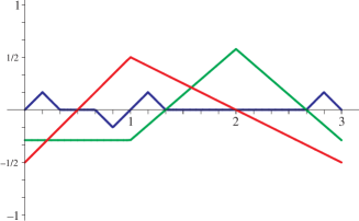
Figure 3.

We have not been able to determine whether (10.11) could be represented as a finite linear combination of shifts of (10.9) and (10.10).

Remark.

We also remark that the solutions (10.7), (10.8) to equation (10.1) with $c=2\cos\theta$ are tropical periodic, hence of finite order two, as soon as $\theta$ is of the form $\theta=2\pi/r$ with $r\in\mathbb{Q}$, while if $\theta$ is an irrational multiple of $2\pi$, then these solutions are non-periodic. However, their order is equal to two, see Theorem 10.3 below.

As a preparation to our final theorem, we add the following observation. Let $y(x)$ be an arbitrary tropical meromorphic solution of

$$y(x+1)+y(x-1)=2(\cos\theta)y(x)$$ (10.12)

with $\theta\in(0,\pi)$. In this case, the solutions $a,b$ of $\lambda^{2}-(2\cos\theta)\lambda+1=0$ are $\cos\theta\pm i\sin\theta$, and so equation (10.3) now takes the form

$$y(x+1)-(\cos\theta+i\sin\theta)y(x)=(\cos\theta-i\sin\theta)(y(x)-(\cos\theta+i\sin\theta)y(x-1)).$$

Denoting $g(x)=s(x)+it(x):=y(x)-(\cos\theta+i\sin\theta)y(x-1)$, we see that $g(x)$ is $1$-periodic in the sense of $g(x+1)=(\cos\theta-i\sin\theta)g(x)$. A simple computation now results in

$$\left(\begin{array}[]{c}s(x+1)\\ t(x+1)\\ \end{array}\right)=\left(\begin{array}[]{cc}\cos\theta&\sin\theta\\ -\sin\theta&\cos\theta\\ \end{array}\right)\left(\begin{array}[]{c}s(x)\\ t(x)\\ \end{array}\right).$$ (10.13)

This means, in particular, that the shift $(s(x),t(x))\rightarrow(s(x+1),t(x+1))$ is a rotation, and since the image of $(s[0,1],t[0,1])$ is bounded, the vector $(s(x),t(x))$ remains bounded over the real axis $\mathbb{R}$. Since $y(x)$ is real, we immediately see that

$$s(x)=y(x)-(\cos\theta)y(x-1),\qquad t(x)=(\sin\theta)y(x-1),$$ (10.14)

i.e.

$$\left(\begin{array}[]{c}s(x)\\ t(x)\\ \end{array}\right)=\left(\begin{array}[]{cc}1&-\cos\theta\\ 0&-\sin\theta\\ \end{array}\right)\left(\begin{array}[]{c}y(x)\\ y(x-1)\\ \end{array}\right).$$

Therefore, $y(x)$ is a bounded tropical meromorphic function.

Theorem 10.3.

Let $y(x)$ be a non-trivial tropical meromorphic solution of equation

$$y(x+1)+y(x-1)=cy(x).$$

If $|c|>2$, then $y$ is of hyper-order $\rho_{2}(y)=1$, while if $|c|\leq 2$, then $y$ is of order $\rho(y)=2$.

Proof.

Suppose first that $|c|\leq 2$. By Theorem 10.1(i)(ii), we may assume that $|c|<2$. Differentiating (10.13), we observe that the slope of $y(x)$ remains uniformly bounded in $\mathbb{R}$. Therefore, the multiplicities of poles of $y(x)$ are uniformly bounded as well. By (10.14) and (10.13), we conclude that the number of distinct slope discontinuities is the same in each interval $[n,n+1)$ as in the initial interval $[0,1)$. Therefore, $N(r,y)\asymp\kappa r^{2}$ for some $\kappa>0$, and since $y(x)$ is bounded, we get $\rho_{2}(y)=2$.

Suppose next that $|c|>2$. Recall the proof of Theorem 10.1, see (10.5) and (10.4) there, and fix $a>1,b<1$ as in this proof. If the hyper-order $\rho_{2}(g)\geq 1$, then (10.4) readily implies that $\rho_{2}(y)\geq 1$. On the other hand, by the representation of $y$ in Theorem 10.1(iii), and the fact that $\rho_{2}(e_{a}(x))=1$, we get $\rho_{2}(y)\leq 1$, hence $\rho_{2}(y)=1$. To prove that

$$g(x):=\sum_{j=1}^{q}\beta_{j}e_{b}(x-x_{j})$$

is of hyper-order one, observe that $e_{b}(x-x_{j})$ has no poles and has zeros exactly at $x_{j}+k$, $k\in\mathbb{Z}$, of multiplicity $(1-b)\mathbb{b}^{k-1}$. Since the points $x_{j}$ are distinct, we may fix one of $e_{b}(x-x_{1}),\ldots,e_{b}(x-x_{q})$, say $e_{b}(x-x_{s})$, to conclude that

$$2T(r,g)\geq N(r,g)+N(r,1_{\circ}\oslash g)\geq N(r,1_{\circ}\oslash e_{b}(x-x_{s}))\geq K(1/b)^{r}$$

for some positive constant $K$, completing the proof. ∎

Remark. In a similar way as made above for (10.1), we could also treat the slightly more general equation

$$y(x+1)\otimes y(x-1)^{\otimes d}=y(x)^{\otimes c}\quad\text{i.e.}\quad y(x+1)-c\,y(x)+d\,y(x-1)=0$$

for $c,d\in\mathbb{R}$ with $c^{2}>d$. In fact, the characteristic equation $\rho^{2}-c\rho(x)+d=0$ has two real roots $\lambda_{1}$ and $\lambda_{2}$ with $\lambda_{1}+\lambda_{2}=c$ and $\lambda_{1}\lambda_{2}=d$. We omit these considerations.

11. Discussion

We remark that Sections 3 to 7 open up a number of possibilities for further investigations such as possible tropical counterparts to deficiencies and ramifications, value distribution theory of tropical difference polynomials and uniqueness theory of meromorphic functions, among other issues.

Concerning our applications to ultra-discrete equations, Section 9 and Section 10, have been restricted, essentially, to a couple of specific examples only, avoiding linear ultra-discrete equations that contain tropical addition, as well as non-homogeneous linear equations and tropical non-linear equations.

The topics pointed out here will be treated, we hope, in subsequent papers.

Acknowledgment. The first author is grateful for a possibility to visit Kanazawa University twice in 2009. These short periods enabled us to start preparing and to finishing this paper.