Higgs mass from cosmological and astrophysical measurements

Abstract

For a robust interpretation of upcoming observations from Planck and LHC experiments it is imperative to understand how the inflationary dynamics of a non-minimally coupled Higgs scalar field may affect the degeneracy of the inflationary observables.
We constrain the inflationary observables and the Higgs boson mass during observable inflation by fitting the Hubble function and subsequently the Higgs inflationary potential directly to WMAP5+BAO+SNI We obtain for Higgs mass $m_{Higgs}=143.73^{\,\,\,\,14.97}_{-6.31}$GeV at 95% CL for the central value of top quark mass. We show that the inflation driven by a non-minimally coupled scalar field to Einstein gravity leads to significant changes of the inflationary parameters when compared with the similar constraints from the standard inflation.

1 Introduction

The primary goal of particle cosmology is to obtain a concordant description of the early evolution of the Universe consistent with both unified field theory and astrophysical and cosmological measurements. Inflation is the most simple and robust theory able to explain the astrophysical and cosmological observations, providing at the same time self-consistent primordial initial conditions [1] and mechanisms for the quantum generation of scalar (curvature) and tensor (gravitational waves) perturbations [2].
In the simplest class of inflationary models, inflation is driven by a single scalar field $\phi$ (inflaton) with some potential $V(\phi)$ minimally coupled to Einstein gravity. The perturbations are predicted to be adiabatic, nearly scale-invariant and Gaussian distributed, resulting in an effectively flat Universe.
The WMAP 5-year CMB measurements alone [3] or complemented with other cosmological datasets [4] support the standard inflationary predictions of a nearly flat Universe with adiabatic initial density perturbations. In particular, the detected anti-correlations between temperature and E-mode polarization anisotropy on degree scales [5] provide strong evidence for correlation on length scales beyond the Hubble radius.

Alternatively one can look on inflationary dynamics based on the structure of the Standard Model (SM) of particle physics. Recently, Bezrukov and Shaposhnikov [6] reported the possibility that the SM with an additional non-minimally coupled term of the Higgs field and Ricci scalar can give rise to inflation without the need for additional degrees of freedom already present in SM. The resultant Higgs inflaton effective potential in the inflationary domain allows for a range of cosmologically values for the Higgs boson mass even after the inclusion of the radiative corrections [7, 8, 9, 10, 11]. More precisely, the present cosmological constraints on the Higgs mass are based on mapping between the Renormalization Group (RG) flow and the spectral index of the curvature perturbations emerging from the analysis of WMAP 5-year data complemented with astrophysical distance measurements [4].
However, after the publication of WMAP results, many works devoted to the reconstruction of the inflationary dynamics during observable inflation [13, 14] show the compatibility between WMAP results and the predictions of the standard inflation driven by a single scalar field with some potential $V(\phi)$ which is minimally coupled with Einstein gravity.

In order to have a robust interpretation of upcoming observations from Planck [15] and LHC [16] experiments it is imperative to understand how the inflationary dynamics of a non-minimally coupled Higgs scalar field may affect the degeneracy of the inflationary observables.
In this paper we aim to constrain the inflationary observables and the Higgs boson mass during observable inflation by fitting the Hubble function $H(\varphi)$, and subsequently the Higgs inflationary potential $V(\varphi)$, directly to WMAP 5-year data [3, 4] complemented with geometric probes from the Type Ia supernovae (SN) distance-redshift relation and the baryon acoustic oscillations (BAO) measurements.

2 Perturbations driven by non-minimally coupled scalar field

We briefly review the computation of the power spectra of scalar and tensor density perturbation generated during inflation driven by a single scalar field non-minimally coupled to gravity via the Ricci scalar R [17, 18, 19, 20, 21].
Jordan frame. We start with the generalized action in the Jordan frame [17]:

$$S=\int d^{4}x\sqrt{-g}\left[\frac{1}{2}U(\varphi){\it\bf R}-\frac{1}{2}G(\varphi)(\nabla\varphi)^{2}-V(\varphi)\right]\,,$$ (1)

where $U(\varphi)$ is a general coefficient of the Ricci scalar, $G(\varphi)$ is the general coefficient of kinetic energy and $V(\varphi)$ is the general potential. The generalized $U(\varphi)$R gravity theory in (1) includes diverse cases of coupling.
For generally coupled scalar field $U=(\gamma+\xi m_{Pl}^{-2}\varphi^{2})$ and $G(\varphi)=1$ where $m_{Pl}\simeq 2.4\times 10^{18}$ GeV is the reduced Planck mass and $\gamma$ and $\xi$ are constants. The non-minimally coupled scalar field is the case with $\gamma=1$ while the conformal coupled scalar field is the case with $\gamma=1$ and $\xi=-1/6$. Throughout the paper we take $sign(\xi)=-1$, keeping the same sign convention for $\xi$ as in Ref. [17]. One should note that other authors [21, 22] use the opposite sign for $\xi$. The background equations in a flat Friedmann-Lemaitre-Robertson-Walker (FLRW) cosmology are given by:

$$H^{2}\equiv\left(\frac{\dot{a}}{a}\right)^{2}=\frac{1}{6U}\left(G\dot{\varphi}^{2}+2U-6H\dot{U}\right)\,,~{}~{}~{}$$ (2)

$$\dot{H}=\frac{1}{2U}\left(-G\dot{\varphi}^{2}+H\dot{U}-\ddot{U}\right)\,,$$ (3)

$$\ddot{\varphi}+3H\dot{\varphi}+\frac{1}{2G}\left(G_{\varphi}\dot{\varphi}^{2}-{\it\bf R}U(\varphi)_{,\,\varphi}+2\,V(\varphi)_{,\,\varphi}\right)=0\,,$$ (4)

where $a$ is the cosmological scale factor ($a_{0}=1$ today), $H$ is the Hubble expansion rate, overdots denotes the time derivatives and ${}_{,\varphi}\equiv\partial/\partial\varphi$.
Einstein frame. The conformal transformation to the Einstein frame for the action (1) can be achieved by defining the Einstein metric as [18]:

$$\hat{g}_{\mu,\nu}=\Omega g_{\mu\nu}\,,$$ (5)

where $\Omega=U(\varphi)$ is the conformal factor. The action in the Einstein frame takes the canonical form:

$$S_{E}=\int d^{4}x\sqrt{-{\hat{g}}}\left[\frac{1}{2}{\it\bf\hat{R}}-\frac{1}{2}(\nabla\hat{\varphi})^{2}-\hat{V}(\varphi)\right]\,,$$ (6)

where the new scalar field $\hat{\varphi}$ and the new potential $\hat{V}$ are defined through:

$${\cal S}(\varphi)^{-2}\equiv\left(\frac{{\rm d}\hat{\varphi}}{{\rm d}\varphi}\right)^{2}=\left.\frac{3m^{2}_{Pl}}{2}\left(\frac{U^{\prime}(\varphi)}{U(\varphi)}\right)^{2}+\frac{G(\varphi)}{U(\varphi)}\right|_{\varphi=\varphi(\hat{\varphi})}\hskip 12.80365pt\left.\hat{V}(\varphi)=\frac{V(\varphi)}{U^{2}(\varphi)}\right|_{\varphi=\varphi(\hat{\varphi})}\,.$$ (7)

The Higgs field suppression factor ${\cal S}(\varphi)$ defined in the above equation was first introduced in Ref.[23] in the context of CMB anisotropy generation in non-minimally inflation model to account for the suppression of the Higgs propagator due to non-minimal coupling with gravity.
Decomposing the conformal factor into the background part and the perturbed part:

$$\Omega(x,t)=\Omega(t)\left(1+\frac{\delta\Omega(x,t)}{\Omega(t)}\right)\,,$$ (8)

we get:

$$\hat{a}=a\sqrt{\Omega}\,,\hskip 8.5359pt{\rm d}\hat{t}=\sqrt{\Omega}{\rm d}t\,,\hskip 8.5359pt\hat{H}=\frac{1}{\sqrt{\Omega}}\left(H+\frac{\dot{\Omega}}{2\Omega}\right)\,,\hskip 8.5359pt\hat{\varphi}=\varphi+\frac{\delta\Omega}{\Omega}\,.$$ (9)

In the above relations $\hat{a}$, $\hat{t}$, $\hat{H}$, $\hat{\varphi}$ are respectively the cosmological scale factor, the cosmic time, the Hubble expansion rate and the scalar field in the Einstein frame.

2.1 Cosmological perturbations in the Jordan frame

Scalar perturbations (S). The equation of motion for the Lagrangian (1) is given by [18]:

$$\frac{1}{a^{3}Q_{\rm S}}\left(a^{3}Q_{\rm S}\dot{\cal R}\right)^{\bullet}+\frac{k^{2}}{a^{2}}{\cal R}=0\,,~{}~{}~{}{\rm with}~{}~{}~{}Q_{\rm S}=\frac{\dot{\varphi}^{2}+3\dot{U}^{2}/2U}{(H+\dot{U}/2U)^{2}}\,.$$ (10)

Here $k$ is the comoving and ${\cal R}$ is the intrinsic curvature perturbation of the co-moving hypersurfaces during inflation:

$${\cal R}=\psi-\frac{H}{\dot{\varphi}}\,\delta\varphi\,,$$ (11)

where $\delta\,\varphi$ is the perturbation of the scalar field $\varphi$. Neglecting the contribution of the decaying modes, the scale dependence of the amplitudes of the scalar perturbations can be obtained by integrating the mode equation [24]:

$$u_{k}^{\prime\prime}+\left(k^{2}-\frac{z^{\prime\prime}}{z}\right)u_{k}=0\,.$$ (12)

In the above equation the prime denote the derivative with respect to the conformal time $\eta(a)=\int a(t)^{-1}dt$. For scalar perturbations the term $z^{\prime\prime}/z$ can be written as [21]:

$$\frac{z^{\prime\prime}_{\rm S}}{z_{\rm S}}=(aH)^{2}\left[(1+\delta_{\rm S})(2+\delta_{\rm S}+\epsilon)+\frac{\delta^{\prime}_{\rm S}}{aH}\right]\,,$$ (13)

where

$$z_{\rm S}=a\sqrt{Q_{\rm S}}\,,\hskip 14.22636pt\epsilon=\frac{{\dot{H}}}{H^{2}}\,,\hskip 14.22636pt\delta_{\rm S}=\frac{{\dot{Q}}_{\rm S}}{2HQ_{\rm S}}\,.$$ (14)

Tensor perturbations (T). Tensor perturbations satisfy the same form of equation as Eq.(10) with replacement $Q_{S}\rightarrow Q_{T}=U$ [17]. The scale dependence of the amplitude of tensor (T) perturbations can also be obtained by integrating Eq.(12) taking the term $z^{\prime\prime}/z$ of the form [21]:

$$\frac{z^{\prime\prime}_{\rm T}}{z_{\rm T}}=(aH)^{2}\left[(1+\delta_{\rm T})(2+\delta_{\rm T}+\epsilon)+\frac{\delta^{\prime}_{\rm T}}{aH}\right]\,,$$ (15)

where

$$z_{\rm T}=a\sqrt{Q_{\rm T}}\,,\hskip 14.22636pt\delta_{\rm T}=\frac{{\dot{Q}}_{\rm T}}{2HQ_{\rm T}}\,.$$ (16)

2.2 The equivalence of the perturbations spectra

Introducing the following quantities:

$$\hat{\epsilon} = \frac{d\hat{H}}{d\hat{t}}\,,\hskip 17.07182pt\hat{\delta_{\rm S}}=\frac{d\hat{Q}_{\rm S}/d\hat{t}}{2\hat{H}\hat{Q_{\rm S}}}\,,\hskip 17.07182pt\hat{\delta_{\rm T}}=\frac{d\hat{Q}_{\rm T}/d\hat{t}}{2\hat{H}\hat{Q_{\rm T}}}\,,$$ (17)

$$\hat{Q}_{\rm S} = \left(\frac{d\hat{\varphi}}{\hat{H}}\right)^{2}=\frac{Q_{\rm S}}{U}\,,\hskip 25.6073pt\hat{Q}_{\rm T}=\frac{Q_{\rm T}}{U}\,,$$

and making use of the relations given in Eq.(14), it can shown that both scalar and tensor perturbations in the Jordan frame exactly coincide with those in the Einstein frame [25, 26] implying that power spectra of the cosmological perturbations are invariant under the conformal transformation:

$$\hat{\cal P}_{\rm S}(k)={\cal P}_{\rm S}(k)\,,\hskip 22.76228pt\hskip 11.38092pt\hat{\cal P}_{\rm T}(k)={\cal P}_{\rm T}(k)\,.$$ (18)

The numerical evaluation of the perturbations power spectra involves solving equations (12), (13) and (15) for each value of the wavenumber $k$, the evolution of $|u_{k}|/z_{S,T}$ to a constant value defining the observable power spectra ${\cal P}_{{\rm S,T}}$. Then the scalar and tensor spectral indexes $n_{\rm S,T}$ and the running of scalar spectral index $\alpha_{S}$ at the Hubble radius crossing $k_{*}$ are defined as:

$$n_{\rm S}-1\equiv\left.\frac{d\,{\rm ln}{\cal P}_{\rm S}(k)}{d\,{\rm ln}k}\right|_{k_{*}=aH}\hskip 11.38092ptn_{\rm T}\equiv\left.\frac{d\,{\rm ln}{\cal P}_{\rm T}(k)}{d\,{\rm ln}k}\right|_{k_{*}=aH}\hskip 11.38092pt\alpha_{\rm S}\equiv\left.\frac{d\,n_{\rm S}(k)}{d\,{\rm ln}k}\right|_{k_{*}=aH}$$ (19)

3 Higgs boson as inflaton

Higgs field couplings in the inflationary domain. Higgs boson as inflaton add non-minimal coupling to gravity [22, 7, 8, 9, 10]. Taking Higgs doublet in the form $(1/\sqrt{2})(0,{\it v}+\varphi)$, the part of the general action given in Eq.(1) relevant for inflation is only the scalar part. The quantum corrections due to the effects of particles of the Standard Model interacting with the Higgs boson through quantum loops modify the action coefficients $U$, $G$ and $V$ that in the Jordan frame take the form [10, 12]:

$$U(t) = 1+\xi(t)G^{2}(t)\frac{\varphi(t)^{2}}{m_{Pl}^{-2}}=1+\xi(t)G(t)\frac{m^{2}_{T}}{m^{2}_{Pl}}e^{2t}\,,$$ (20)

$$G(t) = {\rm exp}\left(\int^{t}_{0}dt^{\prime}\gamma(t^{\prime})\right)\,,$$ (21)

$$V(t) = \frac{\lambda(t)}{4}G^{4}(t)((\varphi^{2}(t)^{2}-{\it v}^{2})^{2}\simeq\frac{\lambda(t)}{4}G^{4}(t)m^{4}_{T}\,e^{4t}\,,$$ (22)

where ${\it v}\simeq 246.2$ GeV is the vacuum expectation value for the Higgs, $\lambda$ is the quadratic coupling constant of the Higss boson with the mass $m_{H}=\sqrt{2\lambda}{\it v}$ and $\gamma(t)$ is the Higgs field anomalous dimension. In the above equations the scaling variable

$$t=t(\varphi)={\rm ln}(\varphi/m_{T})\,,\hskip 12.80365pt\varphi(t)=m_{T}e^{t}$$ (23)

normalizes the Higgs field and all the running couplings to the top quark mass scale $m_{T}=171.3\pm 1.1\pm 1.2$ GeV [27]. As the energy scale of inflation is many order of magnitude above the electroweak scale ($\varphi(t)>>{\it v}$), in the right hand side of Eq.(22) the potential was approximated by a quadratic potential $V(\varphi)=\lambda\varphi^{4}/4$  .
The Higgs field suppresion factor ${\cal S}(t)$, the Higgs potential $\hat{V}(t)$ and the first two potential slow-roll (PSR) parameters $\epsilon_{V}$ and $\eta_{V}$ in the Einstein frame are given by:

$${\cal S}^{2}(t)=\frac{2}{m^{2}_{Pl}}\frac{U^{2}(t)}{G(t)U(t)+3U^{2}_{,\,\varphi(t)}}\,,\hskip 12.80365pt\hat{V}(t)=\frac{V(t)}{U^{2}(t)}\,,$$ (24)

$$\epsilon_{V}=\frac{1}{2}m^{2}_{Pl}\left(\frac{V_{,\,\varphi(t)}}{V}\right)^{2}\,{\cal S}^{-2}\,,\hskip 12.80365pt\eta_{V}=2\epsilon+m_{Pl}\frac{\epsilon_{V_{,\,\varphi(t)}}}{\sqrt{2\epsilon_{V}}}\,{\cal S}^{-1}\,.$$ (25)

The amplitude of the scalar (curvature) perturbations at the Hubble radius crossing $k_{*}$ is related to the Higgs potential in the Einstein frame through:

$$A^{2}_{S}=\left.\frac{\hat{V}}{24\pi^{2}m^{4}_{Pl}\epsilon_{V}}\right|_{k_{*}}\,.$$ (26)

We compute the various $t$-dependent running constants, the Higgs field propagator suppretion factor and Higgs field anomalous dimension by integrating the two-loop renormalization group $\beta$-functions for $SU(2)\times S(1)$ gauge couplings ${g^{\prime},g}$, the $SU(3)$ strong coupling $g_{s}$, the top Yukawa coupling $h_{t}$ and the Higgs quadratic coupling $\lambda$, as collected in the Appendix of [29]. For the non-minimal coupling constant $\xi$ we use the $\beta$-function from the Appendix of [30]. At $t=0$, which corresponds to the top quark mass scale, the top Yukawa coupling $h_{t}(0)$ and Higgs quadratic coupling $\lambda(0)$ are fixed by their pole masses [29]. The gauge coupling constants at $m_{T}$ scale are taken from [8]: $g^{2}(0)=0.4202$, $g^{\prime 2}(0)=0.1291$ and $g^{2}_{s}(0)=0.1.3460$. The value of $\xi(0)$ is determined so that at the initial point of the slow roll inflation, $t_{i}$, the non-minimal coupling constant $\xi(t_{i})$ is such that the calculated value of the amplitude of density perturbations given in Eq.(26) agrees with the measured result obtained by WMAP team [4].

Higgs field equations of motion. Hereafter we will work in the Einstein frame dropping the ‘hat’ when express different quantities in this frame. The inflationary dynamics and the cosmological perturbations power spectra are entirely determined by the dynamics of the Higgs field $\varphi(t)$.
By using the transformation relations from Jordan frame to Einstein frame given in Eq.(9), to the leading order in slow-roll approximation ($\ddot{\varphi}<<3H\varphi$, neglecting also the higher powers in $\dot{\varphi}$ ) the general background Eqs. (2) - (4) reduce to [20, 21]:.

$$H^{2} \equiv \left(\frac{\dot{a}}{a}\right)^{2}\simeq\frac{1}{3m_{Pl}^{2}}\left[\frac{\dot{\varphi}^{2}}{U}\,{\cal S}^{-2}+V\right]\,,$$ (27)

$$3H{\dot{\varphi}} \simeq -UV_{,\,\varphi(t)}\,\,{\cal S}^{-2}\,.$$ (28)

It follows that the amount of the expansion from any epoch to the end of the inflation ($\epsilon_{V}=1$) that is controlled by the number of e-folds ${\cal N}$ is:

$${\cal N}=\int^{\varphi_{end}(t)}_{\varphi(t)}d\varphi^{\prime}(t)\frac{3\,H^{2}(\varphi^{\prime}(t))}{F(\varphi^{\prime}(t))}\,.$$ (29)

The CMB angular power spectra. We obtain the CMB temperature anisotropy and polarization power spectra by integrating the mode equation (12) and the Higgs field equations (27) and (28) with respect to the conformal time. We consider wavenumbers in the range [$5\times 10^{-6}-5$] Mpc^-1 needed to numerically derive the CMB angular power spectra and the Hubble crossing scale $k_{*}=0.002$Mpc^-1. At this scale, the value of the Higgs scalar field $\varphi_{*}$ corresponds to ${\cal N}=k_{*}/aH\simeq$ 59 ${\it e}$-folds till the end of the inflation and the value of the scaling parameter is $t_{*}\simeq$37 [7, 8], as indicated by the central value of the amplitude of scalar perturbations measured by WMAP at $k_{*}$ [4]. For each wavenumber $k$ in the above range our code integrates Eqs.(12), (27) and (28) and the $\beta$ functions of the $t$-dependent running constant couplings in the observational inflationary window imposing that $k$ grows monotonically to the wavenumber $k_{*}$, eliminating at the same time the models violating the condition for inflation $0\leq\epsilon_{H}\equiv-{\dot{H}}/H^{2}\leq 1$.
We reconstruct the Hubble expansion rate $H(\phi-\phi_{*})$ from the data by using the Taylor expansion up to the cubic term, equivalent to keeping the first three slow-roll parameters.
For comparison, we compute the CMB angular power spectra in the standard inflation model with minimally coupled scalar field with a general potential $V(\phi)$. The details of this computation can be found in [14].

4 Results

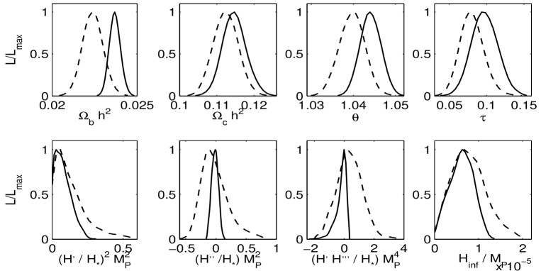
Figure 1: 1D marginalized likelihood probability distributions for seven independent parameters obtained from the fit to WMAP5+SN+BAO dataset of the inflation model with non-minimally coupled Higgs scalar field (continuous lines) and of the standard inflation model with minimally coupled scalar field (dashed lines). The last plot shows the value of Hubble parameter. All parameters are computed at the Hubble radius crossing $k_{*}$=0.002Mpc^-1.

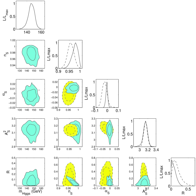
Figure 2: The figure presents the results of the fit to WMAP5+SN+BAO dataset of the inflation model with non-minimally coupled Higgs field in blue (continuous lines) and the results of the fit to the same dataset of the standard inflation model with minimally coupled scalar field in yellow (dashed lines). The top plot in each column shows the probability distribution of different scalar inflationary observables while the other plots show their joint 68% and 95% confidence intervals. All parameters are computed at the Hubble radius crossing $k_{*}$=0.002Mpc^-1.

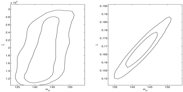
Figure 3: 2D marginalized likelihood probability distributions in the planes $m_{Higgs}$ - $\xi$ (left panel) and $m_{Higgs}$-$\lambda$ (right panel) obtained from the fit to WMAP5+SN+BAO dataset of the inflation model with non-minimally coupled Higgs scalar field.

We use the Markov Chain Monte Carlo (MCMC) technique to reconstruct the Higgs field potential and to derive constraints on the inflationary observables and the Higgs mass from the following datasets.
The WMAP 5-year data [4] complemented with geometric probes from the Type Ia supernovae (SN) distance-redshift relation and the baryon acoustic oscillations (BAO). The SN distance-redshift relation has been studied in detail in the recent unified analysis of the published heterogeneous SN data sets - the Union Compilation08 [32]. The BAO in the distribution of galaxies are extracted from the Sloan Digital Sky Surveys (SDSS) and Two Degree Field Galaxy Redshidt Survey (2DFGRS) [31]. The CMB, SN and BAO data (WMAP5+SN+BAO) are combined by multiplying the likelihoods.
We decided to use these measurements especially because we are testing models deviating from the standard Friedmann expansion. These datasets properly enables us to account for any shift of the CMB angular diameter distance and of the expansion rate of the Universe.

The likelihood probabilities are evaluated by using the public packages CosmoMC and CAMB [33, 34] modified to include the formalism for inflation driven by non-minimally coupled Higgs scalar field, described in the previous sections. Our fiducial model is the $\Lambda$CDM standard cosmological model described by the following set of parameters receiving uniform priors:

$$\Omega_{b}h^{2}\,,\,\,\Omega_{c}h^{2}\,,\,\,\theta_{s}\,,\,\,\tau\,,\,\,A^{2}_{S}\,,\,\,m_{Higgs}\,,\,\,\frac{H^{\prime 2}}{H^{2}}\,,\,\,\frac{H^{\prime\prime}}{H}\,,\,\,\frac{H^{\prime\prime\prime}H^{\prime}}{H^{2}}\,$$

where: $\Omega_{b}h^{2}$ is the physical baryon density, $\Omega_{cdm}h^{2}$ is the physical dark matter density, $\theta_{s}$ is the ratio of the sound horizon distance to the angular diameter distance, $\tau$ is the reionization optical depth, $m_{Higgs}$ is the Higgs boson mass and $H^{\prime}$, $H^{\prime\prime}$ and $H^{\prime\prime\prime}$ are the derivatives of the Hubble expansion rate with respect to the Higgs scalar field.
For comparison, we use the MCMC technique to reconstruct the standard inflation field potential and to derive constraints on the inflationary observables from the fit to WMAP5+SN+BAO dataset of the standard inflation model with minimally coupled scalar field and a general potential $V(\phi)$ [14]. For this case we use the same set of input parameters with uniform priors as in the case of non-minimally coupled Higgs scalar field inflation, except for Higgs mass.
For each inflation model we run 120 Monte Carlo chains, imposing for each case the Gelman & Rubin convergence criterion [35].

Fig. 1 presents the 1D marginalized likelihood probability distributions of the fiducial model parameters obtained from the fit to WMAP5+SN+BAO dataset of the inflation model with non-minimally coupled Higgs scalar field compared with the similar distributions obtained from the fit to same dataset of the standard inflation model with minimally coupled scalar field. One can see the differences between the likelihood probabilities caused by the difference in the dynamics of the scalar fields during inflation. One should note the smaller value of the Hubble expation rate during inflation for the inflation model involving the Higgs field as inflaton.
In Fig. 2 we present the constraints on the inflationary parameters, namely the scalar spectral index $n_{S}$, the running of the scalar spectral index $\alpha_{S}$, the amplitude of the scalar (curvature) density perturbations $A^{2}_{S}$ and the ratio of tensor to scalar amplitudes $R$, as obtained from the fit to WMAP5+SN+BAO dataset of the inflation model with non-minimally coupled Higgs field compared with the constrains obtained from the fit to the same dataset of the standard inflation model with minimally coupled scalar field. We also show the constraints obtained on the Higgs mass from our analysis. The mean values and the 95% CL intervals of these parameters are presented in Table 1.
We obtain a Higgs mass value of $m_{Higgs}=143.73^{\,\,\,\,14.97}_{-6.31}$GeV at 95% CL for the central value of top quark mass.
Our result is compatible with the previous constrains of the Higgs mass from cosmological data [7, 8, 9, 10, 11] however the upper and lower limits of the Higgs mass obtained from this analysis are tightly constrained.
Table 1 clearly show the differences between the estimates of the inflationary parameters obtained from the fits of the inflation models.
Fig 3 shows the 2D marginalized likelihood probability distributions in the planes $m_{Higgs}$ - $\xi$ and $m_{Higgs}$-$\lambda$. One should note the strong correlation between Higgs mass and the Higgs quadratic coupling $\lambda$ and the larger degeneracy between the Higgs mass and non-minimal coupling constant $\xi$, indicating the existence of a degeneracy between $\xi$ and $\lambda$ that affect the Higgs mass value inferred from cosmological and astrophysical measurements.

5 Conclusions

In order to have a robust interpretation of upcoming observations from Planck [15] and LHC [16] experiments it is imperative to understand how the inflationary dynamics of a non-minimally coupled Higgs scalar field may affect the degeneracy of the inflationary observables.
We constrain the inflationary observables and the Higgs boson mass during observable inflation by fitting the Hubble function $H(\varphi)$, and subsequently the Higgs inflationary potential $V(\varphi)$, directly to WMAP 5-year data complemented with geometric probes from the Type Ia supernovae (SN) distance-redshift relation and the baryon acoustic oscillations (BAO) measurements. We obtain a Higgs mass value of $m_{Higgs}=143.73^{\,\,\,\,14.97}_{-6.31}$GeV at 95% CL for the central value of top quark mass $m_{Top}$=171.3 GeV. Our result is compatible with the previous constrains of the Higgs mass from cosmological data [7, 8, 9, 10, 11], however the upper and lower bounds of the Higgs mass obtained from our analysis are tightly constrained.

The strong correlation between Higgs mass and the Higgs quadratic coupling $\lambda$ and the larger degeneracy between the Higgs mass and non-minimal coupling constant $\xi$, indicate the existence of a degeneracy between $\xi$ and $\lambda$ that affect the Higgs mass value inferred from cosmological and astrophysical measurements.

We also show that the inflation driven by a non-minimally coupled scalar field to Einstein gravity leads to significant changes of the inflationary parameters when compared with the similar constraints from the standard inflation with minimally coupled scalar field.

Acknowledgments

The author acknowledge D. Ghilencea for usefull discussions.
This work was partially supported by CNCSIS Contract 539/2009.

Table 1: The mean values and 95% CL lower and upper intervals of the derived parameters obtained from the fit of the inflation model with non-minimally coupled Higgs scalar field and the standard inflation model with minimally coupled scalar field to WMAP5+SN+BAO dataset. All parameters are computed at the Hubble radius crossing $k_{*}$=0.002 Mpc^-1.

Model	Standard Inflation	Higgs Inflation
Parameter
$\Omega_{b}h^{2}$	$0.022_{0.021}^{0.023}$	$0.023_{0.022}^{0.024}$
$\Omega_{c}h^{2}$	$0.111_{0.106}^{0.117}$	$0.114_{0.107}^{0.121}$
$\tau$	$0.082_{0.055}^{0.109}$	$0.094_{0.034}^{0.135}$
$\theta_{s}$	$1.039_{1.034}^{1.045}$	$1.044_{1.037}^{1.048}$
${\rm ln}[10^{10}A^{2}_{S}]$	$3.143_{3.083}^{3.201}$	$3.317_{2.999}^{3.252}$
$n_{S}$	$0.956_{0.932}^{0.979}$	$0.977_{0.944}^{0.997}$
$\alpha_{S}$	$-0.012_{-0.038}^{\,\,\,\,0.021}$	$0.003_{-0.0021}^{\,\,\,\,0.0133}$
$R$	$<0.556$	$<0.234$
$m_{Higgs}$(GeV)		$142.737_{136.431}^{158.707}$
$\lambda$		$0.168_{0.153}^{0.185}$
$\xi\times 10^{-5}$		$1.871_{0.118}^{0.280}$

References

- [1] Starobinsky, A. A. 1979, JETP Lett., 30, 682; Guth, A. H. 1981, Phys. Rev. D, 23, 347; Sato, K. 1981, MNRAS, 195, 467; Linde, A. D, 1982, Phys. Lett.B, 108, 389; Albrecht, A. & Steinhardt, P. J. 1982, Phys. Rev.Lett., 48, 1220; Linde, A. D. 1983, Phys. Lett.B, 129, 177
- [2] Mukhanov, V. F. & Chibisov, G. V. 1981, JETP Lett., 33, 532; Hawking, S. W. 1982,Phys. Lett. B, 115, 295; Starobinsky, A. A. 1982, Phys. Lett. B, 117, 175; Guth, A. H. & Pi S. Y. 1982, Phys. Rev. Lett., 49, 1110; Bardeen, J. M., Steinhardt, P. J. & Turner, M. S. 1983, Phys. Rev. D, 28, 679; Abbott, L. F. & Wise, M. B. 1984, Nucl. Phys. B, 244, 541
- [3] J. Dunkley et al. 2009, ApJS, 180, 306 [arXiv:0803.0586]
- [4] E. Komatsu, et al., 2009, ApJS 180, 330 [arXiv:0803.0547]
- [5] M. Nolta et al. 2009, ApJS, 180, 296 [arXiv:0803.0593]
- [6] F. Bezrukov, M. Shaposhnikov 2008, Phys. Lett. B 659, 703 [arXiv:0710.3755];
- [7] A. O. Barvinsky, A. Yu. Kamenshchik, A. A. Starobinsky 2008, J. CosmologyAstropart. Physics 11, 021 [arXiv:0809.2104];
- [8] A. O. Barvinsky, A. Yu. Kamenshchik, C. Kiefer, A. A. Starobinsky, C. Steinwachs 2009 [arXiv:0904.1698]
- [9] F. L. Bezrukov, A. Magnin, M. Shaposhnikov 2009, Phys. Lett. B 675, 88 [arXiv:0812.4950)]; F. Bezrukov, M. Shaposhnikov 2009, J. High Energy Phys. 07, 089 [arXiv:0904.1537];
- [10] A. de Simone, M. P. Hertzberg, F. Wilczek 2009, Phys. Lett B 678, 1 [arXiv:0812.4946]
- [11] F. Bezrukov, D. Gorbunov, M. Shaposhnikov 2009, J. Cosmology Astropart. Phys. 06, 029 [arXiv:0812.3622]
- [12] A. O. Barvinsky, A. Yu. Kamenshchik, C. Kiefer, A. A. Starobinsky, C. F. Steinwachs 2009, [arXiv:0910.1041]
- [13] R. Easther, and H. V. Peiris 2006, J. Cosmology Astropart. Phys. 09, 010 [arXiv:astro-ph/0604214)]; H. V. Peiris, R. Easther 2006, J. Cosmology Astropart. Phys. 10, 017 [arXiv:astro-ph/0609003]; H. V. Peiris, R. Easther 2006, J. Cosmology Astropart. Phys. 07, 002 [arXiv:astro-ph/0603587]; H. W.Kinney, E. W. Kolb, A. Melchiorri, A. Riotto 2006, Phys. Rev. D 74, 023502 [arXiv:astro-ph/0605338]; J. Lesgourgues, W. Valkenburg 2007, Phys. Rev. D 75, 123519 [astro-ph/0703625]; J. Lesgourgues, A. A. Starobinsky, W. Valkenburg, 2008, J. Cosmology Astropart. Phys. 01, 010 [arXiv:0710.1630];
- [14] L. A. Popa, N. Mandolesi, A. Caramete, C. Burigana 2009, ApJ 706, 1 (in printing) [arXiv:0907.5558]
- [15] N. Mandolesi, M. Bersanelli, C. R. Butler et al. (Planck Collaboration) 2009, Astron. & Astrophys. (submitted)
- [16] G. L. Bayatian et al. (CMS Collaboration) 2007, J. Phys. G34, 995
- [17] R. Fakir and W. G. Unruh, Phys. Rev. D 41 1783 (1990); ibid, Phys. Rev. D 41 1792 (1990).
- [18] Hwang, J. c. 1996, Phys. Rev. D 53, 762 [arXiv:gr-qc/9509044]; Hwang, J. c. & Noh H. 1996, Phys. Rev. D 54, 1460; Noh, H. & Hwang J. c. 2001, Phys. Lett. B 515, 231 [arXiv:astro-ph/0107069]
- [19] E. Komatsu and T. Futamase, nonminimally radiation Phys. Rev. D 58, 023004 (1998) [arXiv:astro-ph/9711340].
- [20] E. Komatsu and T. Futamase, Phys. Rev. D 59, 064029 (1999) [arXiv:astro-ph/9901127].
- [21] Tsujikawa, S. & Gumjudpai, B. 2004, Phys. Rev. D, 69, 123523 [arXiv:astro-ph/0402185]
- [22] T. Futamase and K. Maeda 1989, Phys. Rev. D 39, 399
- [23] D. S. Salopek, J. R. Bond & J. M Bardeen 1989, Phys. Rev. D 40, 1753.
- [24] Mukhanov, V. F. & Chibisov, G. V. 1981, JETP Lett., 33, 532; Mukhanov, V. F. 1985, Zh. Pis’ma v Redaktsiiu 41, 402 (JETP Lett. 41, 493)
- [25] T. Chiba & M. Yamaguchi 2008, J. Cosmology Aspropart. Phys. 10, 021 [astro-ph/0807.4965]; T. Chiba and M. Yamaguchi 2009, J. Cosmology Aspropart. Phys. 01, 019 [astro-ph/0810.5387]
- [26] A. A. Starobinsky 1985, JETP Lett. 42, 152 [Pisma Zh. Eksp. Teor. Fiz. 42 124 (1985)]; M. Sasaki & E. D. Stewart 1996, Prog. Theor. Phys. 95, 71 [arXiv:astro-ph/9507001]; T. T. Nakamura & E. D. Stewart 1996, Phys. Lett. B 381, 413 [arXiv:astro-ph/9604103]
- [27] C. Amsler et al. (Particle Data Group) 2008, Phys. Lett. B 667, 1
- [28] A. R. Liddle, P. Parsons, J. D. Barrow, J. D. 1994, Phys. Rev D 50, 7222 [arXiv:astro-ph/9408015]
- [29] J. R. Espinosa,G. F. Giudice, A. Riotto 2008, J. Cosmology Astropart. Phys. 05, 002 [arXiv:0710.2484]
- [30] T.E. Clark, Boyang Liu, S.T. Love, T. ter Veldhuis 2009, [arXiv:0906.5595]
- [31] W. J. Percival, S. Cole, D. J. Eisenstein, R. C. Nichol, J. A. Peacock, A. C. Pope, A. S. Szalay, S. 2007, MNRAS 381, 1053 [arXiv:0705.3323]
- [32] M. Kowalski et al. (Supernova Cosmology Project) 2008, ApJ 686, 749 [arXiv:0804.4142]
- [33] A. Lewis, & S. Briddle 2002, Phys. Rev. D 66, 103511 [arXiv:astro-ph/0205436]111http://cosmologist.info/cosmomc/
- [34] A. Lewis, A. Challinor, & A. Lasenby A. 2000, ApJ 538, 473[arXiv:astro-ph/9911177] 222http://camb.info
- [35] A. Gelman, & D. Rubin 1992, Statistical Science 7, 457